Sound generated by rubbing objects

Abstract

In the present paper, we investigate the properties of the sound generated by rubbing two objects. It is clear that the sound is generated because of the rubbing between the contacting rough surfaces of the objects. A model is presented to account for the role played by the surface roughness. The results indicate that tonal features of the sound can be generated due to the finiteness of the rubbing surfaces. In addition, the analysis shows that with increasing rubbing speed, more and more high frequency tones can be excited and the frequency band gets broader and broader, a feature which appears to agree with our intuition or experience.

Rubbing objects is an everyday experience. People who have gone through cold winters may have rubbed hands to get warm. Rubbing also occurs in Nature. The earthquake rupture is one of the most familiar but disastrous ones. A common observation is that rubbing can generate sound or noise. The sound generated by rubbing hands is certainly common to nearly every one. The sound generation by ice floe rubbing in the Arctic ocean contributes significantly to the ocean ambient noisePT ; Xie , and may also help sea animals in finding appropriate holes or breaking segments in ice to breath. The sound generated by rubbing scoops against frying pans, however, is likely something most people would like to avoid.

In the present paper, we wish to consider the sound generated by rubbing two finite objects. A model is proposed for the sound generation due to the roughness of the contacting surfaces of the two objects. The sound field is calculated and is analyzed for its relation to the roughness and the rubbing speed. It is shown that sound field can be expressed in terms of a series of eigen-mode excitations, leading to tonal features. It is suggested that when the rubbing speed is low, only low frequency modes are possibly excited. With increasing speed, more and more high frequency modes can be excited, making the frequency spectrum broader. These features appear to be in accordance with our intuition or daily experience.

Consider the problem of two object rubbing. The conceptual layout is shown in Fig. 1. One of the surfaces is moving with a constant velocity along the positive $y$ axis, while the other is assumed to be at rest. For simplicity, we assume that the two objects are identical; for different sizes, the effective rubbing surface will equal that of the smaller one. The shape of the objects is a cubic with thickness $L$, width $W$ and height $H$ along the $x$-, $y$-, and $z$-th axes respectively.

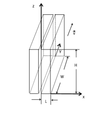
Figure 1: Conceptual layout of the system.

When rubbing occurs, a shear displacement field will be generated at the surfaces and is revealed as the shear waves. Such shear waves can leak out through defects or radiate out at the boundaries, and transform into the sound we hear or record by machines, e. g. microphones.

The governing equation for the shear waves inside the objects is

$$\left(\frac{\partial^{2}}{\partial t^{2}}-c_{s}^{2}\nabla^{2}\right)u(x,y,z,t)=0,$$ (1)

where $c_{s}$ is the shear speed of the objects.

The boundary conditions are Bre

$$\left.\frac{\partial u}{\partial z}\right|_{z=0,H}=0,\ \ \left.u\right|_{y=0,W}=0,$$ (2)

and

$$\left.\frac{\partial u}{\partial x}\right|_{x=L}=0,\ \ \left.\mu\frac{\partial u}{\partial x}\right|_{x=0}=F(y,z,t),$$ (3)

where $\mu$ is the shear modulus of the material.

The stress can be separated into two parts: the mean and the variation, i. e. $F(t,y,z)=\langle F(t,y,z)\rangle+\Delta F(y,z,t)$; here $\langle\cdot\rangle$ denotes the ensemble average. We assume that $\langle F(t,y,z)\rangle$ is independent of $y,z$. It can be shown that the averaged stress can only excite the uninteresting zero-mode, and will thus be ignored.

By Fourier transformation,

$$u(x,y,z,t)=\int d\omega e^{-i\omega t}\hat{u}(x,y,z,\omega).$$ (4)

Eq. (1) becomes

$$(\nabla^{2}+k^{2}_{s})\hat{u}(x,y,z,\omega)=0,$$ (5)

with

$$k_{s}=\frac{\omega}{c_{s}}.$$

The general solution to Eq. (5) with Eqs. (2) and (3) is

$$\hat{u}(x,y,z,\omega)=\sum_{n=0,m=0}^{\infty}A_{mn}\cos(k_{mn}(x-L))\sin(k_{m}y)\cos(k_{n}z),$$ (6)

where

$$k_{n}=\frac{n\pi}{H},\ \ k_{m}=\frac{m\pi}{W},\ \ k_{mn}=\sqrt{k_{s}^{2}-k_{m}^{2}-k_{n}^{2}},$$

and $m,n$ are positive integers.

The coefficient $A_{mn}$ is determined from

$$\sum_{m,n}k_{mn}A_{m,n}\sin(k_{mn}L)\sin(k_{m}y)\cos(k_{n}z)=\frac{1}{\mu}F(\omega,y,z).$$ (7)

Then $A_{mn}$ is solved as

$$A_{mn}=\frac{4}{HW[1+\delta_{n,0}][1+\delta_{m,0}]}\frac{1}{k_{mn}\sin(k_{mn}L)}\frac{1}{\mu}\int_{0}^{H}dz\int_{0}^{W}dyF(\omega,y,z)\sin(k_{m}y)\cos(k_{n}z),$$ (8)

with $F(\omega,y,z)=\frac{1}{2\pi}\int dte^{i\omega t}F(t,y,z).$ It is easy to verify that $\langle A_{mn}\rangle$, caused by the averaged stress, is proportional to $\delta_{n,0}\delta_{m,0}.$ Therefore only zero modes are possible for constant stresses. We will not discuss this situation.

The purpose to calculate the intensity of the shear field which is related to the relevant sound field. That is, we need calculate the correlation function

$$D(x,y,z,t;x^{\prime},y^{\prime},z^{\prime},t^{\prime})\ \equiv\ \langle u(x,y,z,t)u^{\star}(x^{\prime},y^{\prime},z^{\prime},t^{\prime})\rangle.$$ (9)

From the above derivation, it is clear that the key is to find the correlation function of the fluctuation part of the stress at the surface, $\langle\Delta F(y,z,t)\Delta F(y^{\prime},z^{\prime},t^{\prime})\rangle$. Obviously the fluctuation is caused by the roughness of the contacting surfaces. If we assume that the roughness is homogeneous and completely random, i. e. spatially uncorrelated at different point when the system is at rest. When the surface is moving against each other along the $y$-axis, the spatial separation along this direction is correlated at a later time determined as $\Delta/v$. This consideration leads to

$$\langle\Delta F(y,z,t)\Delta F(y^{\prime},z^{\prime},t^{\prime})\rangle=S\delta(z-z^{\prime})\delta(y-y^{\prime}-v(t-t^{\prime})),$$ (10)

where $S$ is a strength factor.

Applying Eq. (10), the intensity field can be calculated. The procedure is to substitute Eqs. (6) and (8) into Eq. (4), then calculate Eq. (9) by taking into account of Eq. (10). We finally get

$$<u(x,y,z,t)u^{\star}(x,y,z,t)> = S\int d\omega\sum_{n}\cos^{2}(k_{n}z)\sum_{m,m^{\prime}}\cos(k_{mn}(x-L))\sin(k_{m}y)\cos(k_{m^{\prime}n}(x-L))\sin(k_{m^{\prime}}y)\times$$ (11)

$$\frac{H}{2}C_{mn,m^{\prime}n}\frac{k_{m}}{(\frac{\omega}{v})^{2}-k_{m}^{2}}\left((-1)^{m}e^{i\frac{\omega}{v}W}-1\right)\frac{k_{m^{\prime}}}{(\frac{\omega}{v})^{2}-k_{m^{\prime}}^{2}}\left((-1)^{m^{\prime}}e^{i\frac{\omega}{v}W}-1\right).$$

This equation can be rewritten as

$$<u(x,y,z,t)u^{\star}(x,y,z,t)>=\frac{S}{\mu^{2}}\int d\omega\sum_{n}\cos^{2}(k_{n}z)|Q_{n}(x,y,\omega)|^{2},$$ (12)

where

$$Q_{n}(x,y,\omega)=\sum_{m}\frac{2}{W\sin(k_{mn}L)}\cos(k_{mn}(x-L))\sin(k_{m}y)\frac{k_{m}}{(\frac{\omega}{v})^{2}-k_{m}^{2}}\left((-1)^{m}e^{i\frac{\omega}{v}W}-1\right).$$ (13)

Therefore the frequency spectrum of the sound intensity field generated by rubbing is

$${\cal P}(\omega)=\frac{S}{\mu^{2}}\sum_{n}\cos^{2}(k_{n}z)|Q_{n}(x,y,\omega)|^{2},$$ (14)

with $Q_{n}$ being given by Eq. (13).

A few general features can be observed from the spectral formula. First, the strength factor $S$ controls the overall sound intensity level. It is expected to depend on a few parameters of the surfaces, such as the friction coefficients and the mechanical properties of the surfaces. Second, due to the factor $\sin(k_{mn}L)$ in the denominator of $Q_{n}$, the resonance feature is expected to appear when $\sin(k_{mn}L)=0$, leading to the phenomenon of tonal sounds. This also shows that the thickness mainly defines the resonance feature. Next, the rubbing speed $v$ enters $Q_{n}$ in the form of $\omega/v$ in the denominator. For a fixed frequency, the decreasing of moving speed will reduced the strength of $Q_{n}$. Therefore with decreasing speed, high frequency components tend to decay accordingly. Furthermore, since $k_{mn}=\sqrt{(\omega/c_{s})^{2}-(m\pi/W)^{2}-(n\pi/H)^{2}}$, the cut-off frequencies are determined by $(\omega/c_{s})^{2}-(m\pi/W)^{2}-(n\pi/H)^{2}\geq 0.$ These features comply with the intuition or experience. It is apparent that the present model can be extended to consider other rubbing surfaces, by adjusting the correlation function of the surface stress. All these features deduced from the theory tend to support the experimental observation of the sound generated by ice-floe rubbingXie . We note that the experimental results have been interpreted by an alternative model Ye .

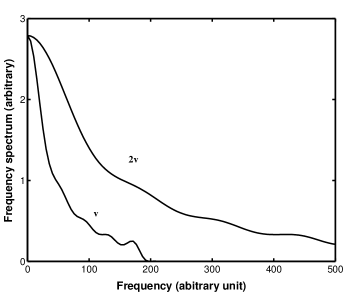
Figure 2: Frequency spectra for two rubbing speeds.

To quantify our discussion, let us consider an example. Suppose that $W=H$, $L=0.1W$, and $S$ is a constant. Two moving speeds are considered: $v/c_{s}=1/600$ and $1/300$. As an example, we compute the sound field located at $(L,W/2,0)$. The frequency spectra for the two moving speed are presented in Fig. 2. The units are arbitrary. Here it is clearly shown that there is indeed a cut-off frequency at about 200 for the lower speed curve. Also for the lower speed case, the discussed resonance feature does appear. For the higher moving speed, the spectrum is broader. But the resonance tends to be weaker. And the cut-off frequency is larger (not shown). Compared to the lower speed case, the frequency band is obviously broader. All these support the above qualitative analysis.

In summary, a model is established to investigate the sound generated by rubbing two objects. In the model, we have assumed that the contacting surfaces are rough and the roughness is described as completely random. The dependence of the frequency spectrum on the moving speed and sample geometries is discussed. The results seem to be in line with intuition or experience.

References

- (1) I. Dyer, Phys. Today 41(1), 5 (1988).
- (2) Y. Xie and D. Farmer, J. Acoust. Soc. Am. 91, 1423 (1992).
- (3) L. M. Brekhovskikh, Waves in Layered Media, (Academic, New York, 1980).
- (4) Z. Ye, J. Acoust. Soc. Am. 97, 2191 (1995).