Alternans amplification following a two-stimulations protocol in a one-dimensional cardiac ionic model of reentry: from annihilation to double-wave quasiperiodic reentry.

Abstract

Electrical pacing is a common procedure that is used in both experimental and clinical settings for studying and/or annihilating anatomical reentry. In a recent study [Comtois and Vinet, Chaos 12, 903 (2002)], new ways to terminate the one-dimensional reentry using a simple protocol consisting of only two stimulations were discovered. The probability of annihilating the reentrant activity is much more probable by these new scenarios than by the usual local unidirectional block. This paper is an extension of the previous study in which the sensitivity of the new scenarios of annihilation to the pathway length is studied. It follows that reentry can be stopped over a limited interval of the pathway length and that increasing the length beyond the upper limit of this interval yields to a transition to sustained double-wave reentry. A similar dynamical mechanism, labeled alternans amplification, is found to be responsible for both behaviors.

I Introduction

The picture of a fixed waveform traveling at constant speed around a ring of excitable tissue, is still a common representation of functional reentry in the clinical setting, particularly in reference to common atrial flutter Mines1914_On ; Frame1988_Os ; Frame1991_Sp ; Pinto1993_En ; Jalil2003_Ex . However, the findings that complex reentries are possible even in a simple homogeneous one-dimensional ionic loop model and that their occurrence is dependent on the steepness of the restitution curve of the action potential duration has altered the current understanding of the phenomena Courtem1993_In ; Vinet1994_Th ; Vinet1999_Me ; Vinet2000_Qu , in which reentry was postulated to remain stable and periodic as long as there was a minimal excitable gap ahead of the wavefront. These findings have also altered the thinking about the effect of antiarrhythmic drugs. Garfink2000_Pr ; Qu2000_Me .

Overdrive pacing using a transvenously inserted catheter in the right atrium is a standard clinical procedure to interrupt atrial flutter.  It is very successful, particularly when it is applied in conjunction with the administration of class I or III antiarrhythmic drug DellaBe1991_Us ; Heldal1993_Ef The use of rapid pacing is likely to increase with the implant of permanent single or dual site stimulator for the prevention of atrial tachycardiasPrakash1997_Ac . However, the mechanism by which overdrive pacing interrupts reentry and the electrophysiological parameters of the reentry circuit that may determined an optimal choice of parameters for the pacing protocol are not understood.

As a first step to improve the pacing algorithm, we have previously studied of a simple protocol of stimulation consisting of two electrical stimuli applied in the pathway of a periodic reentry Comtois2002_Re . New scenarios of reentry annihilation were identified, different from the classical unidirectional block Quan1991_Te ; Shaw1995_Th ; Fei1996_As , which is still considered to be the most important mode of termination.

These alternative scenarios of reentry annihilation follow from a spatiotemporal process that we have called alternans amplification Comtois2002_Re . The first objective of this paper is to understand the effect of length of the reentry pathway on these scenarios of annihilation. We also show that beyond a critical length of the reentry pathway, alternans amplification induces a transition double-wave reentry instead of annihilation.

II Models and methods

Results obtained with two different models are presented. The first model (ionic loop: IL) is a one-dimensional reaction diffusion system, using a cardiac ionic model to represent the transmembrane currents. The second model is an integral-delay equation (ID) based on the local properties of propagation and repolarization.

II.1 Ionic loop model

The well-known monodomain cable equation for an 1D homogeneous excitable cardiac tissue embedded in an unbounded external medium of negligible resistivity is:

$$\frac{1}{\rho}\frac{\partial^{2}V}{\partial x^{2}}=S\left(C_{M}\frac{\partial V}{\partial t}+I_{ion}+I_{stim}\right),$$ (1)

where $V$ is the transmembrane potential (mV), $C_{m}$ is the membrane capacitance ($1\ \mu$Fcm^-2), $S$ the surface-to-volume ratio ($0.4\ \mathcal{\mu}$m^-1, assuming cylindrical cells with radius of $5\ \mathcal{\mu}$m) and $\rho$ is the intracellular resistivity ($200\ \Omega$cm). $I_{ion}$ is given by a modified version of the Beeler-Reuter model (MBR) of the cardiac cell membrane, whose details and space-clamp dynamics are given in Vinet1994_Ex .

For each time step ($\Delta t=2\mu s)$, the system becomes a second order ordinary differential equation that is computed with a Galerkin finite element method projected on a linear basis function and a regular spatial mesh ($\Delta x=50\ \operatorname{\mu m}$)Vinet1994_Th . The resulting tridiagonal linear system of equations is solved with a simplified LU decomposition method. The choice of $\Delta t$ and $\Delta x$ is motivated by the fact that depolarization is the stiffest part of the process. Programs were written in Fortran77 and ran on SGI workstations (Silicon Graphics).

Following the generation of an action potential, two quantities are measured at each site to analyze the propagation: the activation time ($T_{act}(x)$) and repolarization time ($T_{rep}(x)$). $T_{act}(x)$ corresponds to the onset of the action potential and is defined as the moment at which $dV/dt$ reaches its maximum during the upstroke of the action potential. $T_{rep}(x)$ is meant to indicate the time from which a new action potential can be generated by an incoming activation front or an external stimulus. A large set of simulations of sustained reentry in loops of different lengths has showed that an active propagating response was generated if stimulation was applied at least$\ 30$ ms after the$\ -50$ mV post-upstroke downcrossing in repolarization. Accordingly, this instant (i.e. 30 ms after $-50$ mV crossing) is taken as $T_{rep}(x)$. The action potential ($A\left(x\right)$) is defined as the time interval from $T_{act}(x)$ to $T_{rep}(x)$, such that $T_{rep}(x)=T_{act}(x)+A(x)$. The diastolic interval ($D\left(x\right)$) associated to an activation occurring at $T_{act}(x)$ is defined as the time between the previous $T_{rep}(x)$ and current $T_{act}(x)$. With these definitions, a site is excitable if $D\left(x\right)\geq 0$.

II.2 Integral-delay model

The integral-delay model used in this study is an extension of a previous formulation that was developed to describe sustained unidirectional propagation on the loop Courtem1996_A ; Vinet2000_Qu ; Comtois2002_Re ; comtoispre2003 . A first relation $A^{SP}(D)$ gives the duration of the action potential as a function of $D$ in the space-clamped configuration. If the nodes were disconnected from their neighbors, the repolarization time following an activation occurring at $T_{act}(x)$ would be:

$$T_{rep}^{SP}\left(x\right)=T_{act}\left(x\right)+A^{SP}\left(D\left(x\right)\right)$$

provided that $D\geq 0$. If $D<0$, the node is unexcitable. The actual repolarization time of a node at position $x$ is expressed as a weighted average of $T_{rep}^{SP}\left(x\right)$ over a symmetric neighborhood of length $2\alpha$, i.e.:

$$T_{rep}\left(x\right)=\int_{-\alpha}^{\alpha}w\left(u\right)T_{rep}^{SP}\left(x+u\right)du$$

where , $w\left(x\right)=\vartheta^{-1}\exp\left(-\beta x^{2}\right)$ with ($\vartheta=0.5$, $\beta=800$ cm^-2, $\alpha=0.5$ cm), is the weighting function representing the effect of resistive coupling on the repolarization phase. $\beta$ controls the spatial decay of the weighting function and $\vartheta$ is a normalization coefficient such that $\int_{-\alpha}^{\alpha}w\left(u\right)du=1$. The calculation of $T_{rep}$ associated to one excitation is performed at each node at the next instance when it is stimulated by an incoming front or an external stimulus. At this moment, the $T_{rep}^{SP}$ associated to the previous excitation of each point of the neighborhood are collected and averaged to produce $T_{rep}$. In this way, a front whose propagation stops at some location still produces a continuous distribution of $T_{rep}$  around the region of block since $T_{rep}$ is an weighted average of the $T_{rep}^{SP}$  of the sites excited by the front that is blocked and of those that were not reached by that front and still have the $T_{rep}^{SP}\left(x\right)$ associated to their previous excitation. It provides at once a representation of the acceleration of repolarization of the excited cells induced by the load of those that are not excited, and of the prolongation of repolarization in those that were not excited by the electrotonic depolarization induces by the proximal excited cells.

Once the $T_{rep}$ associated to the last excitation that we label $T_{rep}^{last}(x),$ has been computed, the diastolic interval associated to the current stimulation, which take place at the time $T_{act}(x)$, is calculated as:

$$D\left(x\right)=T_{act}\left(x\right)-T_{rep}^{last}(x)$$ (2)

If $D\geq 0,$the stimulus produces an action potential, which propagates on both side with a conduction time $c_{t}(D(x)),$ and reached the neighbouring nodes at the time $T_{act}\left(x\pm\Delta x\right)=T_{act}\left(x\right)+\Delta x$ $c_{t}(D(x))$. If $D<0$, the point is not activated, and its $T_{rep}^{SP}\left(x\right)$ is not changed.

The integral-delay model was originally developed to represent the propagation of  a single activation front during reentry, without external stimulation. In this context, $T_{rep}^{last}(x)$ is always the repolarisation associated to the previous passage of the activation front  and it can be written as $T_{rep}(x-L)=\int_{-\alpha}^{\alpha}w\left(u\right)T_{rep}^{SP}\left(x-L+u\right)du=\int_{-\alpha}^{\alpha}w\left(u\right)(T_{act}\left(x-L+u\right)+A^{SP}\left(D\left(x-L+u\right)\right)du$. Similarly, $T_{act}\left(x\right)=T_{act}\left(x-L\right)+\int_{o}^{L}c_{t}(D(u))du$. With these relations, eq. 2, becomes:

$$D\left(x\right) =T_{act}\left(x\right)-T_{rep}\left(x-L\right)$$ (3)

$$=T_{act}\left(x-L\right)-\int_{-\alpha}^{\alpha}w\left(u\right)T_{act}\left(x-L+u\right)du$$

$$+\int_{0}^{L}c_{t}(D(u))du-\int_{-\alpha}^{\alpha}w\left(u\right)A^{SP}\left(D\left(x-L+u\right)\right)du$$

If the conduction time is constant $\int_{-\alpha}^{\alpha}w\left(u\right)T_{act}\left(x-L+u\right)du=T_{act}\left(x-L\right),$ and eq. 2 is equivalent to the version of the ID model introduced in Vinet2000_Qu . In fact this version neglects the effect of the delay of propagation in calculating the effect of coupling on repolarization. If  $w\left(u\right)$ is taken as a $\delta$ function, which is equivalent to ignoring the effect of coupling, eq. 2  corresponds to the version of  the integral-delay model of Courtemanche and al.
The simulation of the ID model were performed using

$$c_{t}\left(D\right)=c_{t,\min}+17.645e^{-D/2.79}+12.40e^{-D/15.34}$$ (4)

where $c_{t,\min}=14.09$ ms/cm, $D$ is in ms and $c_{t}$ is in ms/cm, and

$$A^{SP}\left(D\right)=42.23+\left[A_{0}-B_{0}e^{-D/\tau}\right]\frac{\left(D+30\right)^{4.92}}{F^{4.92}+\left(D+30\right)^{4.92}}$$ (5)

with $A_{0}=225.22$ ms, $B_{0}=105.74$ ms, $\tau=94.71$ ms, and $F=59.38$ ms Vinet2000_Qu ; Comtois2002_Re . These functions were obtained by fitting the data gathered from different regimes of propagation (free running periodic and QP reentry obtained with the IL model)Vinet2000_Qu . Computations were performed with a spatial discretization of $\Delta x=50$ $\operatorname{\mu m}$, as in the ionic model.

II.3 Protocol of stimulation

For the IL model, $I_{stim}$ consists of a 2.5 ms current pulse applied over an interval of 450 $\operatorname{\mu m}$ with amplitude of 60 $\mathrm{\mu}$A/cm². Dual stimulations were applied on periodic reentry. The timing of  stimuli was controlled by two parameters: $\Delta_{F-S1}$, the time interval between the last activation at the center of the stimulated area and the onset of the first stimulus $S_{1}$; $\Delta_{S1-S2}$ , the time interval between the onset of $S_{1}$ and that of the second stimulus $S_{2}$

For the ID model, the value of $D$, defines the response of the nodes that are stimulated. If $D<0$, the stimulus is applied in the refractory period and doest not have an effect. If $D\geq 0$, the stimulus depolarizes the tissue, defining $A^{SP}(D)$, and induces bi-directional propagation. As for the IL model the stimulation covers 450 $\operatorname{\mu m}$.

III Results

The post-stimuli dynamics are constrained by the steady states of the system. For loops longer than a minimum length $L_{\min}$, sustained reentries are stable attractor of the system. These sustained reentries can be either periodic (period-1) or quasiperiodic (QP), and hold a single (SW), two (DW) or more traveling activation fronts. Table 1 lists the stable solutions of both the ID and IL models for $L<3L_{\min}$. The number and nature of the sustained reentries change with $L$ and condition the outcomes of the stimulations.

Interval	Reentry type
$L$  (cm)	SW (single wave)	DW(double wave)
$0\leq L<L_{\min}=12.8$	$-$	$-$
$L_{\min}\leq L<L_{\min}^{\text{mode-1}}=15.2$	QP, mode-0	$-$
$L_{\min}^{\text{mode-1}}\leq L<L_{crit}=19.5$	$\begin{array}[c]{c}\text{QP},\text{mode-0}\\ \text{QP},\text{mode-1}\end{array}$	$-$
$L_{crit}\leq L<2L_{\min}=25.6$	period-1	$-$
$2L_{\min}\leq L<2L_{\min}^{\text{mode-1}}=30.4$	period-1	$\text{QP},\text{mode-0}$
$2L_{\min}^{\text{mode-1}}\leq L<2L_{crit}=39$	period-1	$\begin{array}[c]{c}\text{QP},\text{mode-0}\\ \text{QP},\text{mode-1}\end{array}$
$2L_{crit}\leq L<3L_{\min}$	period-1	period-1

Table 1: Stable reentries of the IL model as a function of the length of the loop.

QP reentries are characterized by a spatial oscillation of $D$, with a wavelength $\Lambda$ that is an irrational fraction of $L$ (fig. 1A and C). For both SW and DW reentries, there is an interval of $L$ in which two different QP solutions coexist. These solutions, labeled mode-0 and mode-1, have a similar structure but $\Lambda^{\text{mode-0}}\approx 3\Lambda^{\text{mode-1}}$. In SW reentries, the passage of each activation front is associated with a profile of $A$ and $D$ holding one (mode-0, panel A) or multiple (mode-1, panel C) maxima and minima over two turns. For DW QP reentries, $L$ is twice the value for SW QP reentries,  such that mode-0 has one maximum and one minimum over one turn. (fig. 1A). Successive activations at each site alternate between long and short $A$ and $D$ values, except at a number of nodes corresponding to the boundaries from which the phase of the alternation is inverted. As illustrated by the time-course of $T_{act}(x)$ and $T_{rep}(x)$(fig. 1, right panels), the quasi-periodic nature of the propagation makes the position of the extrema and of the nodes to drift slowly in the direction inverse to the propagation of the activation fronts. QP reentry is thus constituted by discordant alternans Watanab2001_Me ; Fox2002_Io ; Echebar2002_In with boundaries between short and long APD moving around the loop.

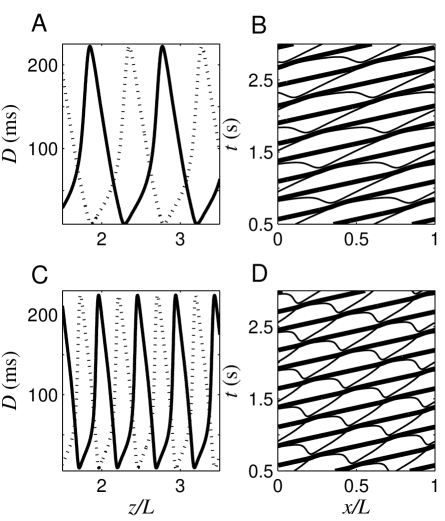
Figure 1: IL model: the mode-0 (panels A-B) and mode-1 DW  reentry (panels C-D) coexisting at $L=34$ cm. In this case, two fronts $F_{1}$ and $F_{2}$ travels along the loop. Left panels: the ordinate gives the value of $D$ at which activation occurs at each site when it is reached by the activation fronts ($F_{1}$, continuous line and $F_{2}$, dotted line). Each site is activated first by $F_{1}$, and later by $F_{2\text{.}}$The abscissa is the distance travelled by the fronts from the same arbitrary reference point (divided by $L$). Right panels: successive $T_{act}\left(x\right)$ (thick line) and $T_{rep}\left(x\right)$ (thin line) at each site. Each successive set of lines corresponds alternatively to the $T_{act}\left(x\right)$ and $T_{rep}\left(x\right)$ profiles associated to $F_{1}$and $F_{2}$. The locations of $F_{1}$ and $F_{2\text{ }}$at any time $t$ are the two positions where $T_{act}\left(x\right)=t$. The successive values of  $D$ at one location are the differences between $T_{act}\left(x\right)$ and the preceding $T_{rep}\left(x\right)$.

Period-1 SW reentry can be annihilated by an isolated stimulus applied in the narrow vulnerable window in which the stimulation produces only a retrograde front, corresponding to the well-known mechanism of unidirectional block Starobi1994_Vu ; Shaw1995_Th ; Fei1996_As . In a previous paper, we have also described other modes of annihilation as well as different transient dynamics that were induced by two successive stimuli Comtois2002_Re . These new modes of annihilation were compatible with experimental observations, and relevant to antiarrhythmic pacing therapy Mensour2000_In . However, that study was restricted to a specific length of the loop ($L_{crit}<L=25$ cm $<2L_{\min}$). In the following, we present a systematic investigation of the outcomes of double stimuli applied on period-1 SW reentry as a function of the timing of the pulses and the length of the loop.

III.1 Functional heterogeneity of refractoriness

Complex dynamics can be induced by a second stimulus $S_{2}$ thanks to the asymmetric profile in $T_{rep}(x)$ left by the interaction of first stimulus $S_{1}$ with the reentry activation front $F$. When $\Delta_{F-S1}$, the time between the last passage of $F$ and the onset of $S_{1}$, is beyond the vulnerable window, $S_{1}$ produces both a retrograde ($R_{1}$) and an antegrade ($A_{1}$) activation front. As illustrated in fig. 2A, the key factor determining the dynamics that can be induced by $S_{2}$ is the region located between the site of stimulation ($x_{S}$) and the site of the collision between $F$ and $R_{1}$ ($x_{c}$, identified by the arrow in 2A). $T_{rep}$ (thin line in fig. 2A) is minimum near $x_{S}$ and reaches its maximum at $x_{c}$. The IL and ID models produce the same profile of $T_{rep}(x)$ (thin lines and triangles, respectively, in 2A), showing that the ID model that was initially developed to describe sustained reentry also provides an appropriate low-dimensional representation of the dynamics when stimulations are applied. The location of $x_{c}$ as well as the profile of $T_{rep}(x)$ around $x_{S}$ depend on both $\Delta_{F-S1}$ and $L$. Figure 2B shows the profile of $T_{rep}(x)$ obtained from loops of different lengths stimulated at the same diastolic interval $D_{S1}(x_{s})=\Delta_{F-S1}(L)-A_{F}(L)$, where $A_{F}(L)$ is the action potential duration of the stable reentry for each $L$. The position of $x_{c}$ is shifted to the left (arrows in 2B) because the collision is delayed on longer loops. However all the loops have the same invariant profile of $T_{rep}$ in the time and space interval that they share before the collision. If $S_{1}$ is applied at larger $D_{S1}$ value, the distance between $x_{S}$ and $x_{c}$ is shortened, $A(x_{S})$ and $T_{rep}(x_{S})$ are increased, such that the extent and depth of the cusp in $T_{rep}$ around $x_{S}$ are diminished.

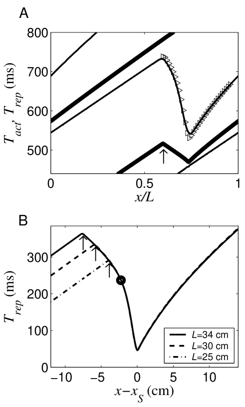
Figure 2: A) $T_{act}(x)$(thick line) and $T_{rep}(x)$ (thin line: IL model, ${\large\vartriangleright}$: ID model) following the application of a stimulus $S_{1}$ at a site $x_{s}$ on a loop of 23 cm holding a period-1 SW reentry. $S_{1}$ produces an antegrade front $A_{1}$ propagating to the right, and a retrograde front $R_{1}$ that collides with the front at the reentry at the site $x_{c}$ indicated by the arrow. B) $T_{rep}(x)$ around the stimulation site $x_{S}$ for loops of  25, 30 and 34 cm, using the ID model. $\Delta_{F-S1}$ was chosen such that $D(x_{S})=\Delta_{F-S1}-A_{F}(L)$ was the same on all loops, $A_{F}(L)$ being the duration of the action potential of the reentry for each case. $x_{c}$ ($\uparrow$) is shifted to the left for longer $L$. The circle indicated the site where $\left|dT_{rep}/dx\right|=$ $c_{t,\max}$.

III.2 Initiating a second antegrade propagation

The spatial profile of $T_{rep}$ for short $\Delta_{F-S1}$ is asymmetrical, with a sharp gradient between $x_{S}$ and $x_{C}$, and a more gradual increase at the right of $x_{S}$. Owing to this asymmetry, the outcome of $S_{2}$ depends on $\Delta_{S1-S2}$, the time interval between the onset of the two stimuli. Figure 3 illustrates a case in which $S_{2}$ is applied after the collision of $F$ and $R_{1}$, at an instant where $A_{1}$, the antegrade front created by $S_{1}$, still has not reached $x_{c}$. $S_{2}$ creates both an antegrade ($A_{2}$) and a retrograde ($R_{2}$) front, but $R_{2}$ is blocked between $x_{S}$ and $x_{c}$. Thereupon, the system is left with two antegrade fronts ($A_{1}$ and $A_{2}$). This occurs as long as $R_{2}$ does not propagate beyond $x_{c}$ to collide with $A_{1}$, in which case $A_{2}$ is left alone to perpetuate the reentry. This is an alternate scenario of unidirectional block that creates a propagating wave in the same direction as $F$ and $A_{1}$.

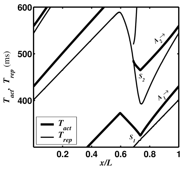
Figure 3: IL model, on a loop of 23 cm: $S_{2}$ creates both an antegrade ($A_{2}$) and a retrograde front $R_{2}.R_{2}$ is blocked between $x_{S}$ and $x_{c}$ shortly after its creation in the refractory tail left by the retrograde front $R_{1}$produces by $S_{1}$.

All the complex dynamics occur in the range of $\Delta_{S1-S2}$ for which $R_{2}$ is blocked between $x_{S}$ and $x_{c}$ whereas $A_{2}$ propagates. This depends on the profile of $T_{rep}\left(x\right)$ left by $S_{1}$, which was shown to be an invariant function of $D_{S1}$ in fig. 2B. Figure 4 shows the global characteristics of the dynamics in the [$D_{S1,}\Delta_{S1-S2}$ ] parameters plane for two values of $L$ ($L=25cm<2L_{\min}$ and $2L_{\min}^{\text{mode-1}}<L=34$ cm $<2L_{crit}$). The parameter plane can be divided in three areas. In the region labeled $\varnothing$ at low $\Delta_{S1-S2}$ values, $S_{2\text{ }}$is applied during the refractory period and does not produce a response. In the upper region, labeled ”$R_{2}\rightarrow$”, $R_{2}$ propagates beyond $x_{c}$, collides with $A_{1}$, and $A_{2}$ is left alone to maintain the reentry. In the middle area, $R_{2}$ is blocked between $x_{c}$ and $x_{s}$and complex dynamics may occur. The phase plane area in which $R_{2}$ is blocked, for $D_{S1}$, between $0$ and $\sim 50$ ms (dotted vertical line), is the same for the two $L$. The specific subsets in which complex dynamics occurs (represented by different shaded areas in fig. 4) change with $L$, and are discussed later.

The article is focused on the area where $R_{2}$ is blocked, between $D_{S1}=0$ and $\approx 50$ ms. The lower limit of the area coincides with $A\left(D_{S1}\right)$ and is close to the action potential duration restitution curve $A^{SP}\left(D\right)$. The upper limit is nearly a constant, around $\Delta_{S1-S2,\max}\approx 204$ ms. Appendix A shows that this $\Delta_{S1-S2}$ upper limit is set by the locus between $x_{s}$ and $x_{c}$ where $|dT_{rep}\left(x\right)/dx|$ is equal to the maximum conduction time. This locus, indicated by a circle for the specific $D_{S1}$ illustrated in 2B, does not depend on $L$, which explains why the upper limit for the block of $R_{2}$ is identical in the two loops. $|dT_{rep}\left(x\right)/dx|$ remains everywhere below the maximum conduction time if $D_{S1}$ is too long, explaining why the area of complex dynamics disappears beyond $D_{S1}$ $\approx 50$ ms. It is also demonstrated in Appendix A that the maximum slope of the $A^{SP}\left(D\right)$ function must be greater than $\sim 1$ to allow the block of $R_{2}$. The same condition that controls the stability of the period-1 reentry Courtem1996_A ; Cytrynb2002_St ; comtoispre2003 thus determines if complex dynamics can be induced by $S_{2}$.

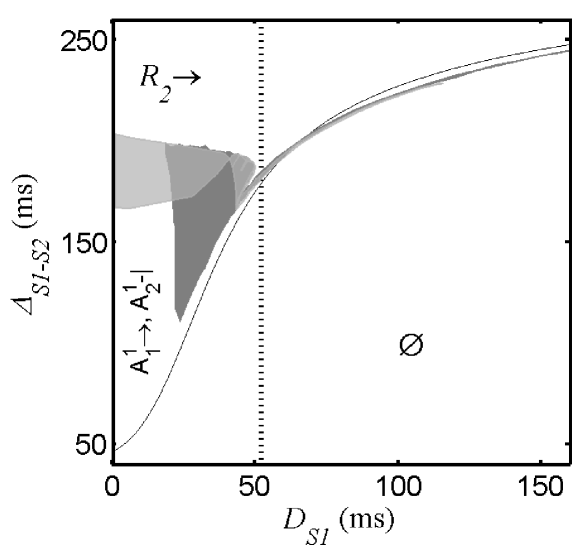
Figure 4: IL model: Outcome of the $S_{1}-S_{2}$ protocol applied on a SW period-1 reentry in the [$D_{S1},\Delta_{S1-S2}$] plane for two loops with $L=25$  and $34$ cm. The two loops have a common lower Region ($\varnothing$) where  $S_{2}$ is applied in the refractory period, and upper region ( $R_{2}\rightarrow$) where $R_{2}$ propagates beyond $x_{c}$. In the area in between, $R_{2}$ is blocked and complex dynamics may occur. They take place in a specific subset for each $L$: $L=25$ cm, ligth gray, $L=34$ cm, dark gray.

III.3 Interactions between the two antegrade propagating fronts

Once $A_{2}$ has started to propagate and $R_{2}$ has been blocked, there are 4 possible outcomes:

1) $A_{1}$ is blocked and $A_{2}$ perpetuates the SW reentry,

2) $A_{2}$ is blocked, and $A_{1}$ maintains the SW reentry,

3) $A_{1}$ and $A_{2}$ are blocked, and reentry is annihilated

4) neither $A_{1}$ nor $A_{2}$ are blocked, and there is a transition to DW reentry. As seen in table 1, this last option can only occur if $L\geq 2L_{\min}$.

The next section discusses the cases 3) and 4) in which the system does not return to the original SW period-1 reentry.

III.3.1 Reentry annihilation by alternans amplification ($A_{1}$ and $A_{2}$ are blocked)

The three new scenarios of reentry annihilation reported in Comtois2002_Re are shown in fig. 5. These scenarios of termination differ in the number of revolution made by the $A_{1}$ and $A_{2}$activation fronts before they are blocked. Accordingly, we introduce the notation $A_{i}^{m}\dashv$ , meaning that the front $A_{i}=\{1,2\}$ is blocked ($\dashv$) after $m$ turns around the loop. Let consider the simplest case ([$A_{1}^{1}\dashv,A_{2}^{1}\dashv$], fig. 5A) in which both $A_{1}$ and $A_{2}$ are blocked after one rotation. $A_{1}$ is blocked first near $x_{S}$, when it reaches the refractory tail left by $A_{2}$ and $R_{2}$. This occurs because $A_{1}$ has already completed a fraction of its rotation when $S_{2}$ is applied. As a consequence, $A_{1}$ comes back to reactivate the sites near $x_{S}$ after a time interval much shorter than the period of rotation $T$ of the stable reentry. The block of $A_{2}$ takes place between $x_{c}$ and the site where $R_{2}$ was blocked. When $A_{1}$ travels in this zone, the region has last been excited by $R_{1}$, and a time interval longer than $T$ has elapsed since this last excitation. Besides, both the action potential and $T_{rep}$ associated to $R_{1}$ were short since $S_{1}$ was premature. As a consequence, $A_{1}$ produces action potentials that are longer than those of the stable reentry. Since the time between the passage of $A_{1}$ and the return of $A_{2}$ is also shorter than $T$, $A_{2}$ is blocked. The block of $A_{2}$ thus results from a process of amplified alternation in a region between $x_{S}$ and $x_{c}$. The premature $R_{1}$ that creates short action potential is followed by the late $A_{1}$ generating long action potential.

In the two other scenarios, $A_{1}$ nor $A_{2}$ are blocked after either 2 or 3 turns ([$A_{1}^{2}\dashv,A_{2}^{2}\dashv$], [$A_{1}^{3}\dashv,A_{2}^{3}\dashv$] in fig. 5B-C). Each passage of $A_{1}$ leaves around $x_{S}$ a convex profile of $T_{rep}$, which is turned to a concave profile by the subsequent passage of $A_{2}$. The panel B and C illustrates the process of alternans amplification. Alternans amplification may end up by the blockade of one of the front, in which case propagation reverts to SW reentry. It may saturated, leading to DW reentry, or may lead to annihilation. The next section explores the conditions for annihilation.

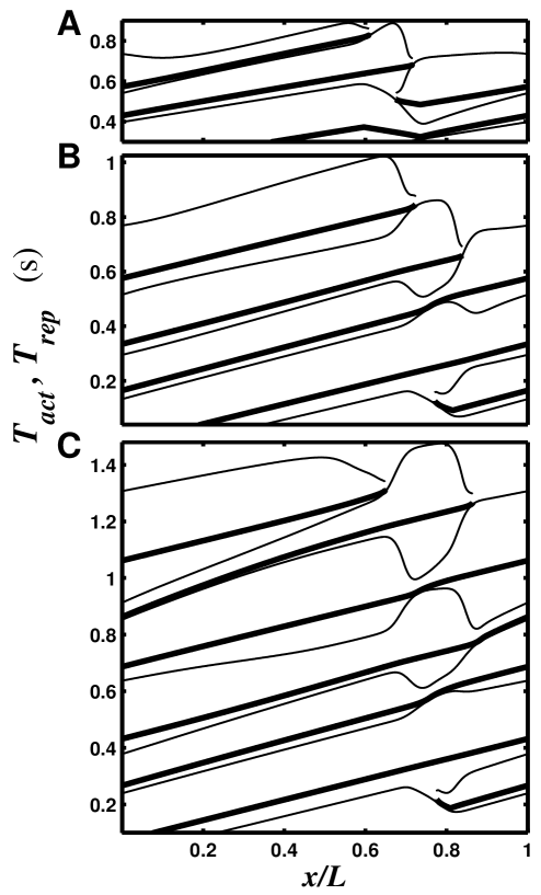
Figure 5: IL model: profile of $T_{act\text{ }}$(thick line) and $T_{rep}$ (thin line) for the three different scenarios of annihilation caused alternans amplification model in the ring. A) $L=23$ cm, $D_{S1}=10$ ms, $\Delta_{S1-S2}=160$ ms, [$A_{1}^{1}\dashv,A_{2}^{1}\dashv$], B) $L=25$ cm, $D_{S1}=47$ ms, $\Delta_{S1-S2}=190.4$ ms, [$A_{1}^{2}\dashv,A_{2}^{2}\dashv$], C) $L=25$ cm, $D_{S1}=47$ ms, $\Delta_{S1-S2}=185.1$ ms [$A_{1}^{3}\dashv,A_{2}^{3}\dashv$]. $S_{1}$ and $S_{2}$ are pictured in panel A, but only $S_{2}$ is shown in panel B and C.

The scenarios of annihilation by alternans amplification occurs over limited range of $L$

The conditions leading to each type of alternans amplification annihilation vary with $L$, and none exists for $L$ $>$$\sim 30.5$ cm. The four panels of fig. 6 picture the extent of the different zones of annihilation for $L$ ranging from $L_{crit}=19.5\operatorname{cm}$, the minimum $L$ with stable period-1 SW reentry, to the limiting $L\approx 30.5$ cm value. At short $L$ ($L=20.5$ $\operatorname{cm}$, fig. 6A), there is a large [$D_{S1}$, $\Delta_{S1-S2}$] area with [$A_{1}^{1}\dashv,A_{2}^{1}\dashv$] block located at low $D_{S1}$ values, and a small adjacent area of [$A_{1}^{2}\dashv,A_{2}^{2}\dashv$]  block. The zone of [$A_{1}^{2}\dashv,A_{2}^{2}\dashv$]  always remains minimal; and it is the first to disappear at $L\approx 28.5$ cm. The zone of [$A_{1}^{3}\dashv,A_{2}^{3}\dashv$] appears at intermediate $L$, expands, and is the last to disappear.

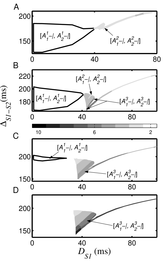
Figure 6: IL model: Area with complex dynamics and alternans amplification in the ($D_{S1},$ $\Delta_{S1-S2})$ plane with A to D) $L=20.5$, $25.0$, $27.5$, $28.5$ cm.  The gray scale indicates the number of turns during which $A_{1}$ and $A_{2}$ persist together. The regions with different annihilation are specified accordingly. Otherwise, one front ends up being blocked and propagation reverts to period-1 SW reentry.

Disappearance of the [$A_{1}^{1}\dashv,A_{2}^{1}\dashv$] annihilation

Taken together, the maps of fig. 4 and fig. 6 A-C shows that the area of [$A_{1}^{1}\dashv,A_{2}^{1}\dashv$] is embedded in the larger region, invariant with respect to $L$, in which $R_{2}$ is blocked between $x_{c}$ and $x_{S}$. The zone of [$A_{1}^{1}\dashv,A_{2}^{1}\dashv$] is located at intermediate $\Delta_{S1-S2}$, just over the area, labeled [$A_{1}^{1}\rightarrow,A_{2}^{1}\dashv$] (fig. 4), in which $A_{1}$can propagated beyond $x_{S}$, but $A_{2}$ is stopped by the refractory tail left by $A_{1}$. As $L$ is increased, the lower boundary of [$A_{1}^{1}\dashv,A_{2}^{1}\dashv$] is lifted, thus diminishing the [$A_{1}^{1}\dashv,A_{2}^{1}\dashv$] area until it disappears completely. The lost of [$A_{1}^{1}\dashv,A_{2}^{1}\dashv$] annihilation is thus caused by the inability of the system to block $A_{1}$ at its first return.

Appendix B provides the conditions needed for $A_{1}$ to block in the tail of $A_{2}$ and proves that there is a limiting $L$ beyond which this cannot happen. To summarize: 1) Increasing $\Delta_{S1-S2}$ produces longer action potential for $S_{2}$, delays $T_{rep}(x_{S})$, and thus augments the likelihood of $A_{1}$ to be blocked. 2) However, the increase of $\Delta_{S1-S2}$ and $T_{rep}(x_{S})$ are bounded by the condition of $R_{2}$ being blocked between $x_{S}$ and $x_{c}$, and these limiting values are independent of $L$. 3) Since increasing $L$ delays the return of $A_{1}$, there is a length $L$ from which the return of $A_{1}$ always occurs after the limiting $T_{rep}(x_{S})$ value.

Opening the way to more than one rotation for both fronts

Figure 6 shows that, for each value of $L$, the zone of [$A_{1}^{1}\dashv,A_{2}^{1}\dashv$]  and [$A_{1}^{2,3}\dashv,A_{2}^{2,3}\dashv$] blocks are disjoint, being respectively located at low and high $D_{S1}$. As seen in fig  6D, the zones of [$A_{1}^{2,3}\dashv,A_{2}^{2,3}\dashv$] remain located at large $D_{S1}$ even at values of $L$ for which [$A_{1}^{1}\dashv,A_{2}^{1}\dashv$]  does not exists anymore. However, enlarging $L$ also leads to the appearance and extension of areas in which $A_{1}$ and $A_{2}$ persist together for an increasing number of turns before one of the front is blocked (up to 7 activations in 6D). As $L$ is increased, the areas of the parameters plane associated to these other forms of transient complex dynamics extend toward low $D_{S1}$, to finally cover all the range from $D_{S1}=0$ to $50$ ms when $L=37.5$ cm, a value close to $2L_{crit}$ from which DW reentry becomes possible. The areas of the parameters plane associated to these behaviors with coexistence of  $A_{1}$ and $A_{2}$ for multiple turns form a sequence of contiguous parallel tongues.

All the higher modes of block and complex dynamics require that both $A_{1}$ and $A_{2}$ travel beyond $x_{s}$, at least at their first return. Conditions for the block of $A_{2}$ are derived in Appendix C based on an approximation using the $A^{SP}\left(D\right)$ equation and rules for $A_{1}$ and $A_{2}$ return cycles. It shows that the block of $A_{2}$ depends on the balance between the return cycle of $A_{1}$ and $A_{2}$.

III.3.2 Transition to double-wave reentry (neither $A_{1}$ nor $A_{2}$ is blocked)

In both the ID and IL model, annihilation by alternans amplification is impossible from $L$ $\geq$ 30.5 cm. In fact, for 31 $>L\ \geq$ 30.5 cm, only transient complex dynamics with a final return to period-1 SW reentry are observed. However, the maximum number of turns with $A_{1}$ and $A_{2}$ co-traveling grows, just as the number of tongues in the [$D_{S1},\Delta_{S1-S2}$ ] plane associated to different numbers of turns during which the two fronts coexist. Each new tongue appears at low $D_{S1}$ and $\Delta_{S1-S2}$ values, and expands as $L$ is further increased. Finally, a first transition to QP mode-0 DW reentry is detected at $L=31$ cm (fig. 7A). Transition to DW reentry thus appears as the asymptotic limit of the prolongation of the transient propagation with two fronts. However, transition to DW reentry begins much beyond $L=2L_{\min}$ $=25.6$ cm, the value at which sustained mode-0 QP DW reentry starts to exist. In fact, at $L=31$ cm, the system is rather in the range of $L$ for which both DW mode-0 and mode-1 solutions coexists.

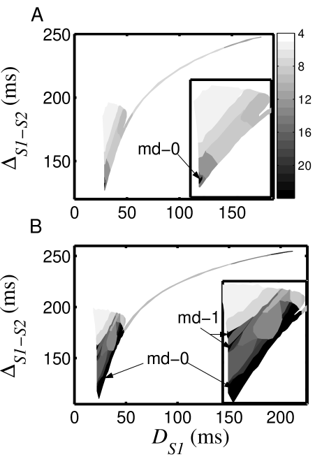
Figure 7: IL model: area of complex dynamics in the $D_{S1}$ vs. $\Delta_{S1-S2}$ plane for $L=31$ cm (panel A) and $L=34$ cm (panel B). The gray code indicates the number of turns during which $A_{1}$ and $A_{2}$ persist together. Arrows pinpoint the zones with transition to mode-0 and mode-1 DW QP dynamics.

For longer $L$, (fig. 7B) the region with transition to mode-0 DW reentry expands, as it was the case for all the zones associated to two fronts transient propagation created at shorter $L$. Transition to mode-1 DW reentry also appears. However, the transition to mode-1 appears at low $D_{S1}$, but at two disjoint intermediate $\Delta_{S1-S2}$ values, giving rise to two separated areas.

For still longer $L$, the areas of mode-0 and mode-1 transition enlarge until covering, from $L=37.5$ cm, all the area where $R_{2}$ is blocked. Hence, from this value of $L,$transition to DW reentry occurs in all instances where $R_{2}$ is blocked. Finally, beyond $2L_{crit}=39$ cm, all transitions go to period-1 DW reentry, which is the only DW solution that remains.

III.3.3 Selecting the mode of QP reentry

Increasing the length of the pathway correlates with an increase in the complexity of the dynamics and to the transition to sustained DW reentry. The results presented in fig. 7 show that changing the timing of the stimuli when $2L_{\min}<L<2L_{crit}$ can induce the transition either to the mode-0 or mode-1 DW QP reentry. The IL model was simulated with $L=37.5$ cm ($2L_{\min}\leq L<2L_{crit}$ but near $2L_{crit}$) to circumscribe the basin of attraction in the parameter space associated to each DW QP reentry. The large area in which two antegrade fronts are created ($D_{S1}<50$ ms) is separated between two regions, with lower $\Delta_{S1-S2}$ converging to mode-0, and higher $\Delta_{S1-S2}$ to mode-1. In this last section, we compare the transient dynamics leading to each of two modes of DW QP reentry.

Figure 8  shows the spatial profile of $D$ associated to $A_{1}$ and $A_{2}$ for two cases converging respectively to mode-0 (panel A) and mode-1(panel B). In this representation,  the passage of $A_{2}$ ($D_{A2}\left(z\right)$, dotted line) at each location is followed by that of $A_{1}$ ($D_{A1}\left(z\right),$full line). At first, $A_{2}$ propagates with a short $D$, producing brief action potentials everywhere along the loop. As a consequence, $A_{1}$ travelling afterwards meets long $D\left(z\right)$. $D_{A1}\left(z\right)$ has its first maximum (P₁) when it travels between $x_{c}$ and the point where $R_{2}$was blocked, such that $D_{A2}$ has a minimum at the same location from which it increases slowly until its next return in the same region. From there, $D_{A2}\left(z\right)$ starts to alternate between long and short values with a spatial period close to 2 turns, and $D_{A1}\left(z\right)$ follows a complementary profile. This first phase of the propagation, lasting for approximately 8 turns, can be labeled as concordant alternans since $D_{A2}$ and $D_{A1}$ have alternating values and that each remains short or long for at least one complete rotation. This pattern does not correspond neither to mode-0 nor mode-1, since both stabilized DW QP solutions have a wavelength less than $L$.

However, from the beginning ($k=1,2$), $D_{A1}$ already shows a second spatial oscillation in $D$ that is superimposed to the concordant alternans. The structure of this oscillation, which has a wavelength close to one turn, makes the difference between the cases converging to mode-0 and mode-1. In the former case, the oscillation embeds two peaks {P₁, P₂} ($D_{A1}$ for mode-0, continuous line in fig. 8A), while in the later case, it has three peaks {P₁, P₂, P₃} ($D_{A1}$ for mode-1, continuous line in fig. 8B). These superimposed spatial variations persist while the concordant alternans dissipate. During this process, the position of the peaks does not change much. As the amplitude of the concordant alternans decreases, the respective height of the discordant alternans increases up to a point where the boundary with large gradient in $D$ begins to move around the loop due to the quasiperiodic nature of the propagation. This travelling mechanism is akin to the propagation of paced discordant alternans on a cable of cardiac tissueWatanab2001_Me ; Fox2002_Io ; Echebar2002_In .

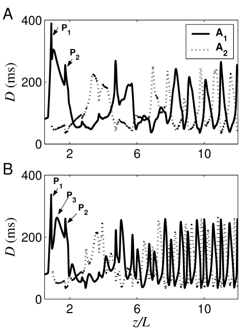
Figure 8: The spatial variation of $D$ as a function of the travelled distance for the transition to A) mode-0 and B) mode-1 double-wave QP reentry.

The main difference between the transition to mode-0 and mode-1 is the presence of the third peak P₃ in $D_{A1}$. The P₃ peak of $D_{A1}$ is induced by the increase of $\Delta_{S1-S2}$. On one hand, a larger $\Delta_{S1-S2}$ produces a longer $T_{rep}$ such that $A_{1}$ meets a lower $D$ and the amplitude of P₁ is reduced. But a larger $\Delta_{S1-S2}$ also implies that $A_{2}$ travels faster, comes back sooner to the stimulation sites, and set the stage for a new maximum in the $D_{A1}$ profile.

Of course the transition from two to three peaks is continuous process since a similar variation of $D$ with less amplitude already exists with the transition to mode-0 in fig. 8A. It means that there must be a minimal spatial profile that corresponds to the boundary between the two basins of attraction (the transition to either mode-0 or mode-1).

IV Discussion

Alternans amplification, leading either to reentry annihilation or transition to DW reentry, can exist if the slope of the APD restitution curve is larger than one. Hence, the condition on the slope of the APD restitution curve that is mandatory for the existence of sustained QP reentrycomtoispre2003 also enables double-pulse stimulation to produce a new mode of unidirectional block, in which only an antegrade front propagates away from the stimulation site. On any closed circuit with two activation fronts travelling in opposite direction, this opens a large spatio-temporal window in which an ectopic focus or an external source firing twice can start a reentry. This is consistent with the use of burst pacing as a standard experimental and clinical procedure to start tachycardia Vinet1996_Cy ; Cao1999_Sp ; Helie2000_Cy ; Nattel2000_Ba . In a loop already holding a SW reentry, the $S_{1}-S_{2}$ protocol can induced the simultaneous propagation of two antegrade fronts whose final outcome depends on the timing of the stimuli and the length of the loop. The transient or persistent coexistence of two antegrade fronts is a new type of dynamics in which the effects of the stimuli cannot be represent as perturbations of a limit-cycle, as it has been done for models in which the steep slope criteria was not fulfill Nomura1996_En ; Glass2002_Pr .

In clinical and experimental investigations, stimulations are currently used to either study the characteristics of reentry circuits through resetting or to stop the tachycardias Fei1996_As ; Jalil2003_Ex . Most often, stimulations are applied at one site and propagation is assessed through one or a few recording electrodes. We may consider the dynamics that will be observed  with this setting for each of the three scenarios of annihilation by alternans amplification. Since the distance traveled by $R_{1}$ from $x_{s}$ to $x_{c}$ usually covers a small portion of the reentry pathway, electrodes are much more likely to be positioned in the complementary portion of the circuit. For [$A_{1}^{1}\dashv,A_{2}^{1}\dashv$],  such electrodes will detect the last passage of $F$ before the collision with $R_{1}$, then $A_{1\text{ }}$and $A_{2}$. The detection of $A_{1\text{ }}$and $A_{2}$ would clearly exclude classical unidirectional block being responsible for the annihilation. In fact, this modeling study was initiated after a set of experimental and clinical studies on flutter using multichannel (4 to 8 channels) recordings Mensour2000_In . In these, cases of annihilation were reported in which $F$, $A_{1\text{ }}$, $A_{2}$ were detected, and in which the propagation of $A_{1\text{ }}$and $A_{2}$ was blocked in the segment of the circuit were the collision of $F$ and $A_{1\text{ }}$was presumed to have occurred. This scenario, that was called collision block, is consistent with the [$A_{1}^{1}\dashv,A_{2}^{1}\dashv$] block by alternans amplification Comtois2002_Re . In the case of [$A_{1}^{2}\dashv,A_{2}^{2}\dashv$] block, $A_{1}$ and $A_{2}$ would be detected twice (see 5B). Since the time intervals from each $A_{1}$ to the next $A_{2}$ are longer than that between $A_{2}$ and the following $A_{1}$, the sequence of the differences between activation times alternates around a value shorter than the period of the original reentry, the block occurring after the longer interval of the time series. For [$A_{1}^{3}\dashv,A_{2}^{3}\dashv$], each front is seen thrice, with similar oscillation in the time series of  the difference. However, the structure of oscillation of the cycle as well as the last value before annihilation depend on the position of the electrode in the circuit. In a protocol for annihilation by unidirectional block, the detection of $A_{1\text{ }}$and $A_{2}$ would indicate that the stimuli were beyond the vulnerable window and would trigger the application of a new stimulus at shorter coupling interval. However, this could rather reinitiate a reentry bound to stop by alternans amplification.

To allow the unidirectional block of $R_{2}$, $S_{1}$ must be applied early beyond the vulnerable window, in the portion of the excitable gap referred as partially refractory by electrophysiologists DellaBe1991_Us ; Heisel1997_Fa . The prematurity of $S_{1}$, in conjunction with the high slope of the APD restitution curve and of the $\theta$ dispersion curve, create a concave asymmetrical profile of $T_{rep}(x)$ around $x_{s}$. For a given $S_{1}$, the $\Delta_{S1-S2}$ intervals for which $R_{2}$ is blocked depends on the local dynamics around $x_{s}$ that is again determined by the APD restitution and the dispersion of $\theta$. In fact, when the parameters $D_{S1}$ is used to describe the timing of the first stimulus, the [$D_{S1},\Delta_{S1-S2}$] range to get a block of $R_{2}$ becomes independent of $L$.

The pivotal role of the $A^{SP}(D)$ and $\theta(D)$functions is further confirmed by the capacity of the ID model to reproduce the dynamics of the ionic model. However, in order to avoid discontinuity in $T_{rep}(x)$ in the region where $R_{2}$ is blocked and get a correct representation of the dynamics, spatial averaging must be included in the computation of the spatial profile of $T_{rep}(x)$. Originally, spatial averaging was added to the ID model to reproduce the modulation of the repolarization by resistive coupling in order to correct the shortcomings of the model regarding the details of the bifurcation from periodic to QP propagation Vinet2000_Qu . Including spatial averaging becomes even more essential when stimulations and blocks produce steep gradients in $T_{rep}(x)$ Comtois2002_Re .

While the wide range of [$D_{S1},\Delta_{S1-S2}$] for which $R_{2}$ is blocked does not depends on $L$, this is not the case for the subset of this interval leading to reentry annihilation by alternans amplification. As shown in fig. 6, the interval of block is very large for $L\simeq L_{crit}$ and decreases gradually until it disappears at $L\simeq 2L_{\min}^{\text{mode-1}}$. For the MBR model used herein, annihilation by alternans amplification exists for $30.5>L>19.4$ cm, and it occurs on a range of [$D_{S1},\Delta_{S1-S2}$] that remains much wider than the $\sim 1$ ms standard vulnerable window for most of this range of $L$. This is consistent with the result of a clinical study in which dual pulses stimulation was found to be four times more effective than single stimulus to stop monomorphic ventricular tachycardia in man Almendr1986_An . As $L$ is increased, the [$D_{S1},\Delta_{S1-S2}$] area of $R_{2}$ block also encloses a growing number of tongues with increasingly prolong coexistence of $A_{1}$ and $A_{2}$, a process that culminates in the appearance of zones of transition to DW reentry. Then the zones with transition to DW reentry extend until they cover completely the area in which $R_{2}$ is blocked. From $L\simeq 2L_{crit},$ blocking $R_{2}$ yields automatically to sustained DW reentry. Hence, transition to DW reentry does not necessarily imply a heterogeneous substrate as it is been proposed elsewhere Brugada1991_On ; Cheng1998_Ac , but can also be achieved in a homogeneous medium through the creation of a functional heterogeneity by a limited number of electrical stimulations. Annihilation and transition to DW occur on separated ranges of loop lengths. On shorter loop, reentry annihilation is produced when alternans amplification reaches an amplitude high enough to block $A_{1}$and $A_{2}$. On longer loop, the distributed alternans saturate at an amplitude that still permits sustained propagation. In our version of the BR model, the transition from SW QP to period-1 reentry at $L_{crit}$ is supercritical. However, we have shown that, for other sets of parameters, the bifurcation is subcritical, with bistability between QP and period-1 reentry near $L_{crit}$ Vinet1999_Me . In these cases, it is possible that the two-stimulations protocol applied to the SW period-1 reentry near $L_{crit}$ could induced a transition to SW QP propagation, a phenomenon that was not possible with the instance of the MBR model used in this paper.

Our results are consistent with different clinical and experimental observations, and open the possibility to design more effective anti-arrhythmic pacing strategies. However, the modeling studies must be extended to more realistic representations to evaluate properly potential applications. Preliminary results from an ongoing work on a two-dimensional annulus show that block by alternans amplification can still be obtained on this setting, but that additional scenarios are possible, including termination through transient fibrillation that has also been observed in real cardiac tissue. Tissue heterogeneity, either at the level of the ionic properties or of the cells coupling, could also be important since termination of reentry has been obtained in a one-dimensional loop model embedding a small area of slower conduction but using an ionic model with minimal APD restitution properties Sinha2002_Cr ; Sinha2002_Te . It remains to be seen if annihilation based on alternans amplification would be amplified or reduced by the inclusion of spatial inhomogeneity. Investigation will also have to be extended to bidomain model in order to get a more proper representation of the stimulus. The simplified representation used herein can be an acceptable approximation for low amplitude stimuli or to mimic the effect spontaneous firing of a group of cells. However it is known that current spread of the stimulus depend on the properties of the external and internal medium Lindblo2000_Ro ; Keener2003_Th . The MBR representation of the ionic properties is also oversimplified. However, since most phenomena described in this paper occurs in the few first beat after the stimulations and can be explained from the APD restitution and speed dispersion, it is unlikely that slow memory effects appearing in the dynamics of more complex model would change the behaviour. Characterizing the APD restitution and speed dispersion of the more complex model in the range of frequency of repetitive activity associated to reentry should allow a prediction of the possible dynamics.

V Conclusion

This work is a further illustration of the richness and diversity of the dynamics that can results from the restitution of APD and dispersion of the speed even in a simplified model of the tissue. It has revealed some unexpected behaviours, like block by alternans amplification, which can be much more prevalent than the mechanism of unidirectional block that are usually assumed to be dominant. The low-dimensional model whose behaviour is equivalent to the ionic model, provides a generic understanding of the dynamics that can used a guideline to investigate the effects of future complexification of the model.

Appendix A The upper limit of the $\Delta_{S1-S2}$ interval for double-wave creation

Three conditions must be fulfilled for the block to occur: 1) $R_{2}$, the retrograde front created by $S_{2}$, must be blocked between the stimulation site $x_{s}$and $x_{c},$ the locus of the collision between the reentry front $F$ and retrograde front $R_{1}$ created by $S_{1}$; 2) afterward, $A_{1}$, the antegrade front produced by $S_{1}$, must be blocked when it returns near $x_{s}$; 3) finally, $A_{2}$, the antegrade front produced by $S_{2}$, must also be blocked when it travels between $x_{s}$ and $x_{c}$ The following three appendixes formulate the constraints associated with each of these conditions. In all three appendixes, we consider that $F,A_{1}$and $A_{2}$ travels toward increasing value of $x$, we use $T_{rep,F}(x_{s})$, the repolarization time associated to the passage of the last activation front of the reentry $F$ at $x_{S}$, as the reference time $t=0$, and introduce a spatial coordinate $y=\left(x_{s}-x\right)\geq 0$ to follow the retrograde fronts $R_{1}$ and $R_{2}$.

$R_{2}$ can propagate as long as its activation time $T_{act,R2}(x)$ is larger than $T_{rep,R1}(x)$, the repolarization time associated to $R_{1}$. In the limiting case $T_{act,R2}(x)=T_{rep,R1}(x)$, $D_{R2}(x)=T_{act,R2}(x)-T_{rep,R1}(x)=0$, and $R_{2}$ travels with the maximum conduction time $-dT_{act,R2}/dx=c_{t}\left(0\right)$ =$c_{t,\max}$. When $R_{2}$ reaches a point $x_{c}<x_{0}<x_{s}$ with $D_{R2}(x_{0})=0,$ it can continue to propagate if $\left|dT_{rep,R1}(x_{0})/dx\right|$ $\leq c_{t,\max}$. The limiting case for the propagation of $R_{2}$ is thus

$$T_{rep,R1}(x_{0}) =T_{act,R2}(x_{0})$$ (6)

$$\left|\frac{dT_{rep,R1}(x_{0})}{dx}\right| =c_{t,\max}$$

We neglect the effect of coupling in the calculation of $T_{rep,R1}$ to obtain

$$T_{rep,R1}\left(y\right)\simeq T_{act,R1}(y)+A^{SP}\left(D_{R1}\left(y\right)\right)$$ (7)

where $D_{R1}\left(y\right)=$ $T_{act,R1}(y)-T_{rep,F}(y)$ is the diastolic interval associated to the propagation of $R_{1}$. From our choice of reference time and the definition of $y$, $T_{act,R1}(0)=D_{S1}$. In the MBR model, the $c_{t}$ dispersion curve is very steep such that the conduction time is minimal, except for a short interval of $D$ close to $0$. As a consequence, we approximate that both $R_{1}$ and $F$ have been propagating with the minimum conduction time (i.e. maximum speed) $c_{t,\min}$, such that

$$T_{rep,F}(y) \simeq-c_{t,\min}y$$

$$T_{act,R1}(y) \simeq D_{S1}+c_{t,\min}y$$

$$D_{R1}(y) =T_{act,R1}(y)-T_{rep,F}(y)\simeq D_{S1}+2c_{t,\min}y$$

Substituting these relations in eq. 7 yields

$$T_{rep,R1}\left(y\right)\simeq D_{S1}+c_{t,\min}y+A^{SP}\left(D_{S1}+2c_{t,\min}y\right)$$ (8)

Taking the spatial derivatives of eq. 8 yields

$$\frac{dT_{rep,R1}}{dy}=c_{t,\min}\left(1+2\left.\frac{dA^{SP}}{dD}\right|_{D_{R1}\left(y\right)}\right).$$

which, thanks to eq. 8, gives

$$\left.\frac{dA^{SP}}{dD}\right|_{D_{R1}\left(y_{0}\right)=D_{\max}}=\frac{c_{t,\max}-c_{t,\min}}{2c_{t,\min}}$$

The existence and location of the critical point depends on the slope of the restitution curve, and on the relative difference between the maximum and minimum conduction time. From the $c_{t}(D)$ given by eq. 4 , $c_{t,\max}\simeq 3.13c_{t,\min}$, and

$$\left.\frac{dA^{SP}}{dD}\right|_{D_{R1}\left(y_{o}\right)=D_{\max}}\simeq 1.065.$$ (9)

Using eq. 5 to solve this equation, we obtain that $D_{\max}\approx D_{S1}+2c_{t,\min}y_{0}\simeq 70$ ms. This result means that, if $D_{S1}>D_{\max}\simeq 70$ ms, $\left|dT_{rep,R1}/dx\right|<c_{t,\max}$ everywhere between $x_{c}$ and $x_{s}$, and $R_{2}$ cannot be blocked. It means also that if $D_{S1}<D_{\max}$, there is a critical point $x_{c}<x_{0}<x_{s}$ whose position depends on $D_{S1}$ but is independent of $L$. The last step is to determine the maximum $\Delta_{S1-S2}$ ($\Delta_{S1-S2,\max}$) to get a block of $R_{2\text{ }}$ at the $x_{0}$. Assuming again that $R_{2}$ travels with the minimum conduction time, the first condition of eq. 6 becomes

$$D_{S1}+c_{t,\min}y+A^{SP}\left(D_{\max}\right)=D_{S1}+\Delta_{S1-S2,\max}+c_{t,\min}y$$

reducing to the limit

$$\Delta_{{}_{S1-S2}},_{\max}=A^{SP}\left(D_{\max}\right)$$

The maximum $\Delta_{S1-S2}$ for the block of $R_{2\text{ }}$is independent of $L$ and of $D_{S1}$, provided that .$D_{S1}<D_{\max}$. For $S2$ to induce propagation $\Delta_{S1-S2}$, must also be $\geq APD(D_{S1})$, which is the refractory period at $x_{s}$. In summary, for all $0\leq D_{S1}\leq D_{\max}\simeq 70$ ms, $R_{2}$ blocks if $APD^{SP}(D_{S1})\leq\Delta_{{}_{S1-S2}}\leq A^{SP}\left(D_{\max}\right)$.

The main approximation used herein is that both $R_{1}$ and $R_{2}$ propagate everywhere with the minimal propagation time. With regard to $R_{1}$, the error introduces by the approximation is minimal unless $D_{S1}\simeq 0$. For $R_{2}$, the conduction time is obviously underestimated when its activation time comes close to $T_{rep,R1}$. The approximation thus overestimates $D_{\max}$, whose value is around 50 ms for the ID and IL  model, compared to the $D_{\max}=70$ ms provided by the approximation.

Appendix B Block of $A_{1}$ after one rotation on the loop

Appendix A shows that $\forall D_{S1}\in[0,D_{\max}]$, $R_{2}$ exist and is blocked if $\Delta_{{}_{S1-S2}}\in[APD^{SP}(D_{S1}),A^{SP}\left(D_{\max}\right)],$ a set of conditions that do not depend on $L$. The next event is the annihilation $A_{1}$ when it returns near $x_{s}$ and hits the refractory tail left $A_{2}$. Using $T_{rep,F}(x_{s})$ as a reference time $A_{1}$ comes back to $x_{s}$ at the time $D_{S1}+\tau_{A1}$, in which $\tau_{A_{1}}$ is the time taken by $A_{1}$ to propagates over the loop on its first turn. It is blocked if the system is still refractory, which means

$$T_{rep,S2}>D_{S1}+\tau_{A_{1}}$$ (10)

Neglecting the effect of coupling on repolarization, $T_{rep,S2}$ is approximated as:

$$T_{rep,S2}\simeq D_{S1}+\Delta_{S1-S2}+A^{SP}(D_{S2})$$ (11)

in which $D_{S2}$, the diastolic interval associated to $S_{2}$, is estimated by

$$D_{S2}\simeq\Delta_{S1-S2}-A^{SP}(D_{S1})$$ (12)

Substituting eq. 11 and 12 in eq. 10 yields

$$\Delta_{S1-S2}+A^{SP}(\Delta_{S1-S2}-A^{SP}(D_{S1}))>\tau_{A_{1}}\text{,}$$ (13)

in which $\tau_{A_{1}}$ is the only non- local term. For most ionic models and experimental preparations, $\tau_{A1}$ is a monotonic decreasing function of $D_{S1}$ (as in fig. 4 of ref. Comtois2002_Re ). The effect of the prematurity on the return cycle comes from the steepness of the $c_{t}$ dispersion curve (eq. 4) which is close to $c_{t,\min}$ as soon as $D$ is greater than a few tenths of ms. Therefore, the prolongation of the return cycle depends on the limited region beyond $x_{s}$ over which $A_{1}$ does not propagate at the maximum speed. Hence, we write

$$\tau_{A1}\left(D_{S1},L\right)\approx Lc_{t,\min}+f\left(D_{S1}\right)$$ (14)

where $f$ is maximum for $D_{S1}=0$ and

$$\frac{df}{dD_{S1}} <0,$$

$$\lim_{D_{S1}\longrightarrow\infty}f =0$$

The condition 13 for the block of $A_{1}$ becomes

$$\Delta_{S1-S2}+A^{SP}(\Delta_{S1-S2}-A^{SP}(D_{S1}))>Lc_{t,\min}+f\left(D_{S1}\right)\text{.}$$ (15)

Consider

$$\Delta_{S1-S2}^{\lim}+A^{SP}(\Delta_{S1-S2}^{\lim}-A^{SP}(D_{S1}))=Lc_{t,\min}+f\left(D_{S1}\right)$$ (16)

as the minimum value of $\Delta_{S1-S2}$ to get a block of $A_{1}$.

Lets consider next the case where $D_{S1}<D_{\max}$ and $\Delta_{S1-S2}=A^{SP}(D_{S1})$, for which $D_{S2}=0$. The condition for the block of $A_{1}$ becomes

$$A^{SP}(D_{S1})+A^{SP}(0)=Lc_{t,\min}+f\left(D_{S1}\right)$$

which cannot be fulfilled since both $D_{S1}$ and $A^{SP}(0)$ are smaller than the diastolic interval of the free reentry. The block of $A_{1}$ will occur from the minimum $\Delta_{S1-S2}>A^{SP}(D_{S1})$. This explains why the dynamical regime [$A_{1}^{1}\rightarrow,A_{2}^{1}\dashv$] is found in the lower portion of the [$D_{S1},\Delta_{S1-S2}$] area in which $R_{2}$ blocked, as seen in figure 4.

The condition for the block of $R_{2}$ are that $D_{S1}\in[0,D_{\max}]$ and $\Delta_{{}_{S1-S2}}\in[APD^{SP}(D_{S1}),A^{SP}\left(D_{\max}\right)]$. Since the right hand side of eq. 16 is a growing function of $L$, $\Delta_{S1-S2}^{\lim}$ for any fixed value of $D_{S1}$ must also increase with $L$ until reaching $A^{SP}\left(D_{\max}\right)$. Hence, there is a limit value of $L$ from which $A_{1}$cannot be blocked on its first return. For $D_{S1}^{\lim}(L)$, the value of $D_{S1}$ for which $\Delta_{S1-S2}^{\lim}=APD^{SP}(D_{\max})=\Delta_{S1-S2,\max}$, eq. 16 becomes

$$\Delta_{S1-S2,\max}+A^{SP}(\Delta_{S1-S2,\max}-A^{SP}(D_{S1}^{\lim}(L))=Lc_{t,\min}+f\left(D_{S1}^{\lim}(L)\right)$$

Shortening $D_{S1}^{\lim}(L)$  increases both the left and right side of the equation, such that the value of $D_{S1}^{\lim}(L)$ depends on the balance between the slope of $df/dD$ (i.e. the change in the return cycle) and $dA^{SP}/dD$ (the change in repolarisation time at $x_{s}$). The derivative of the equation with respect to $L$ gives:

$$\left(-\frac{df}{dD_{S1}}-a_{D_{S1}}^{\prime}a_{D_{S2}}^{\prime}\right)\frac{dD_{S1}^{\lim}}{dL}=c_{t,\min}$$

where $a_{D_{0}}^{\prime}=\left.dA^{SP}/dD\right|_{D=D_{0}}$. In the MBR model, $\left|\partial f/\partial D_{S1}\right|<1,$ whereas $dA^{SP}/dD>1$ at low $D$ value, such that $dD_{S1}^{\lim}/dL<0,$ as observed in the numerical simulations.

Appendix C Block of $A_{2}$ after one rotation on the loop

Appendix B  shows that $A_{1}$ is blocked only over a subset of the [$D_{S1},\Delta_{{}_{S1-S2}}$] area for which $R_{2}$ exist and is blocked (i.e. $D_{S1}\in[0,D_{\max}]$, $\Delta_{{}_{S1-S2}}\in[APD^{SP}(D_{S1}),A^{SP}\left(D_{\max}\right)]$). With respect to $\Delta_{{}_{S1-S2}}$, the lower bound of this subset is greater than $APD^{SP}(D_{S1})$ and increases with $L$, while the upper bound remains constant at $A^{SP}\left(D_{\max}\right)$. With respect to $D_{s1},$the variation of the limits of this subset is given by a complex expression that depends on the slope of both the restitution and dispersion curves. For the MBR model, the upper $D_{S1}$ of the subset decreases toward 0 as $L$ is increased. The last step is to obtain the conditions for the block of $A_{2.}$

$A_{2}$ blocks between $x_{c}$ and the locus where $R_{2\text{ }}$has stopped when it hits the refractory tail left by $A_{1}$. Using the $y$ coordinate, the condition for the block of $A_{2}$ is that there is a point where

$$T_{rep,A1}\left(y\right)>T_{act,A2}\left(y\right)$$ (17)

$T_{rep,A1}(y)$ is approximated as $T_{act,A1}\left(y\right)+A^{SP}(D_{A1}\left(y\right),$where $D_{A1}\left(y\right)=T_{act,A1}\left(y\right)-T_{rep,R1}\left(y\right)$ since $R_{2}$ has not propagated in this region. Using eq. 8 of appendix  A  for $T_{rep,R1}(y)$ and eq. 14 of appendix B for $T_{act,A1}\left(y\right)$ yields

$$T_{repol,A1}=D_{S1}+Lc_{t,\min}+f\left(D_{S1}\right)-c_{t,\min}y+A^{SP}(D_{A1}\left(y\right)$$ (18)

$$D_{A1}\left(y\right)=Lc_{t,\min}+f\left(D_{S1}\right)-2c_{t,\min}y-A^{SP}\left(D_{S1}+2c_{t,\min}y\right)$$

$T_{act,A2}\left(y\right)=D_{S1}+\Delta_{{}_{S1-S2}}+\tau_{A2}(y)$ where $\tau_{A2}$ is the time needed for $A_{2}$ to travel from the stimulation site to $y$. For $A_{1}$, we have assumed in B that the prolongation of the return cycle was occurring mainly in a short region around $x_{s}$ beyond which $A_{1}$ was travelling at maximal speed. The situation is different for $A_{2}$. As it could be seen in fig. 5 A, the $D$ associated to $A_{2}$ as it propagates away form $x_{s},$meaning that it speed of propagation diminishes. Nevertheless, we write

$$\tau_{A2}(y)=Lc_{t,\min}+g\left(D_{S1,}D_{s2}\right)-c_{t,\min}y$$ (19)

With eq. 18 and 19, the condition 17  for the block $A_{2}$ after one rotation becomes

$$f\left(D_{S1}\right)+A^{SP}(D_{A1}\left(y\right))>\Delta_{S1-S2}+g\left(D_{S1},D_{S2}\right)$$ (20)

To get the [$A_{1}^{1}\dashv,A_{2}^{1}\dashv$] block, the conditions given by eq. 15 and eq. 20 must both be fulfilled, leading to the final condition:

$$A^{SP}\left(\Delta_{S1-S2}-A^{SP}\left(D_{S1}\right)\right)>Lc_{t,\min}+g\left(D_{S1},D_{S2}\right)-A^{SP}\left(D_{A1}\left(y\right)\right).$$

with the supplementary constraint that $\Delta_{S1-S2}$ and $D_{S1}$ must remain in the interval where $R_{2}$ is block. Since both $\Delta_{S1-S2}$ and $D_{S1}$ are bound, there is a limiting $L$ value beyond which [$A_{1}^{1}\dashv,A_{2}^{1}\dashv$] block cannot occur. For the IL and ID model,   we found that $A_{2}$ was always stop when $A_{1}$ was blocked, meaning that eq. 20  was fulfilled whenever eq. 15 was satisfied. However, the condition depends on the restitution and dispersion curve and, through $g\left(D_{S1},D_{S2}\right)$, the interaction of $A_{2}$ with the spatial profile of $T_{repol}$ left by $A_{1}$.