Damping factors for the gap-tooth scheme

Abstract

An important class of problems exhibits macroscopically smooth behaviour in space and time, while only a microscopic evolution law is known. For such time-dependent multi-scale problems, the gap-tooth scheme has recently been proposed. The scheme approximates the evolution of an unavailable (in closed form) macroscopic equation in a macroscopic domain; it only uses appropriately initialized simulations of the available microscopic model in a number of small boxes. For some model problems, including numerical homogenization, the scheme is essentially equivalent to a finite difference scheme, provided we repeatedly impose appropriate algebraic constraints on the solution for each box. Here, we demonstrate that it is possible to obtain a convergent scheme without constraining the microscopic code, by introducing buffers that “shield” over relatively short times the dynamics inside each box from boundary effects. We explore and quantify the behavior of these schemes systematically through the numerical computation of damping factors of the corresponding coarse time-stepper, for which no closed formula is available.

1 Introduction

For an important class of multi-scale problems, a separation of scales exists between the (microscopic, detailed) level of description of the available model, and the (macroscopic, continuum) level at which one would like to observe the system. Consider, for example, a kinetic Monte Carlo model of bacterial chemotaxis [SGK03]. A stochastic biased random walk model describes the probability of an individual bacterium to run or “tumble”, based on the rotation of its flagellae. Technically, it would be possible to run the detailed model for all space and time, and observe the macroscopic variables of interest, but this would be prohibitively expensive. It is known, however, that, under certain conditions, one can write a closed deterministic model for the evolution of the concentration of the bacteria as a function of space and time.

The recently proposed gap-tooth scheme [KGK02] can then be used instead of performing stochastic time integration in the whole domain. A number of small intervals (boxes, teeth), separated by large gaps, are introduced; they qualitatively correspond to mesh points for a traditional, continuum solution of the unavailable chemotaxis equation. The scheme works as follows: We first choose a number of macroscopic grid points. We then choose a small interval around each grid point; initialize the fine scale, microsopic solver within each interval consistently with the macroscopic initial conditions; and provide each box with appropriate (as we will see, to some extent artificial) boundary conditions. Subsequently, we use the microscopic model in each interval to simulate evolution until time $\Delta t$, and obtain macroscopic information (e.g. by computing the average density in each box) at time $\Delta t$. This amounts to a coarse time-$\Delta t$ map; this procedure is then repeated.

The generalized Godunov scheme of E and Engquist [EE03] also solves an unavailable macroscopic equation by repeated calls to a microscopic code; however, the assumption is made that the unavailable equation can be written in conservation form. In the gap-tooth scheme discussed here, the microscopic computations are performed without assuming such a form for the “right-hand-side” of the unavailable macroscopic equation; we evolve the detailed model in a subset of the domain, and try to recover macroscopic evolution through interpolation in space and extrapolation in time.

We have showed analytically, in the context of numerical homogenization, that the gap-tooth scheme is close to a finite difference scheme for the homogenized equation [SKR03]. However, that analysis employed simulations using an algebraic constraint, ensuring that the initial macroscopic gradient is preserved at the boundary of each box over the time-step $\Delta t$. This requires altering an existing microscopic code, so as to impose this macroscopically-inspired constraint. This may be impractical (e.g. if the macroscopic gradient has to be estimated), undesirable (e.g. if the development of the code is expensive and time-consuming) or even impossible (e.g. if the microscopic code is a legacy code). Generally, a given microscopic code allows us to run with a set of pre-defined boundary conditions. It is highly non-trivial to impose macroscopically inspired boundary conditions on such microscopic codes, see e.g. [LLY98] for a control-based strategy. This can be circumvented by introducing buffer regions at the boundary of each small box, which shield the short-time dynamics within the computational domain of interest from boundary effects. One then uses the microscopic code with its built-in boundary conditions.

Here, we show we can study the gap-tooth scheme (with buffers) through its numerically obtained damping factors, by estimating its eigenvalues. Integration with nearby coarse initial conditions is used to estimate matrix-vector products of the linearization of the coarse time-$\Delta t$ map with known perturbation vectors; these are integrated in matrix-free iterative methods such as Arnoldi eigensolvers. For a standard diffusion problem, we show that the eigenvalues of the gap-tooth scheme are approximately the same as those of the finite difference scheme. When we impose Dirichlet boundary conditions at the boundary of the buffers, we show that the scheme converges to the standard gap-tooth scheme for increasing buffer size.

2 Physical Problem/ Governing Equations

We consider a general reaction-convection-diffusion equation with a dependence on a small parameter $\epsilon$,

$$\frac{\partial}{\partial t}u(x,t)=f\left(u(x,t),\frac{\partial}{\partial x}u(x,t),\frac{\partial^{2}}{\partial x^{2}}u(x,t),x,\frac{x}{\epsilon}\right),$$ (1)

with initial condition $u(x,0)=u_{0}(x)$ and Dirichlet boundary conditions $u(0,t)=v_{o}$ and $u(1,t)=v_{1}$. We further assume that $f$ is 1-periodic in $y=\frac{x}{\epsilon}$.

Since we are only interested in the macroscopic (averaged) behavior, let us define an averaging operator for $u(x,t)$ as follows

$$U(x,t):=\mathcal{S}_{h}(u)(x,t)=\int_{x-\frac{h}{2}}^{x+\frac{h}{2}}u(\xi,t)\mathrm{d}\xi.$$ (2)

This operator replaces the unknown function with its local average in a small box of size $h>>\epsilon$ around each point. If $h$ is sufficiently small, this amounts to the removal of the microscopic oscillations of the solution, retaining its macroscopically varying components.

The averaged solution $U(x,t)$ satisfies an (unknown) macroscopic partial differential equation,

$$\frac{\partial}{\partial t}U(x,t)=F\left(U(x,t),\frac{\partial}{\partial x}U(x,t),\frac{\partial^{2}}{\partial x^{2}}U(x,t),x;h\right),$$ (3)

which does not depend on the small scale, but instead has a dependence on the box width $h$.

The goal of the gap-tooth scheme is to approximate the solution $U(x,t)$, while only making use of the detailed model (1). For illustration purposes, consider as a microscopic model the constant coefficient diffusion equation,

$$\frac{\partial}{\partial t}u(x,t)=a^{*}\frac{\partial^{2}}{\partial x^{2}}u(x,t),$$ (4)

In this case both $U(x,t)$ and $u(x,t)$ satisfy (4). The microscopic and macroscopic models are the same, which allows us to focus completely on the method and its implementation.

3 Multiscale/Multiresolution Method

3.1 The gap-tooth scheme

Suppose we want to obtain the solution of the unknown equation (3) on the interval $[0,1]$, using an equidistant, macroscopic mesh $\Pi(\Delta x):=\{0=x_{0}<x_{1}=x_{0}+\Delta x<\ldots<x_{N}=1\}$. To this end, consider a small interval (tooth, box) of length $h<<\Delta x$ centered around each mesh point, and let us perform a time integration using the microscopic model (1) in each box. We provide each box with boundary conditions and initial condition as follows.

Boundary conditions. Since the microscopic model (1) is diffusive, it makes sense to impose a fixed gradient at the boundary of each small box for a time $\Delta t$ for the macroscopic function $U(x,t)$. The value of this gradient is determined by an approximation of the concentration profile by a polynomial, based on the (given) box averages $U_{i}^{n}$, $i=1,\ldots,N$.

$$u(x,t_{n})\approx p_{i}^{k}(x;t_{n}),\qquad x\in[x_{i}-\frac{h}{2},x_{i}+\frac{h}{2}],$$

where $p_{i}^{k}(x;t_{n})$ denotes a polynomial of (even) degree $k$. We require that the approximating polynomial has the same box averages in box $i$ and in $\frac{k}{2}$ boxes to the left and to the right. This gives us

$$\frac{1}{h}\int_{x_{i+j}-\frac{h}{2}}^{x_{i+j}+\frac{h}{2}}p_{i}^{k}(\xi;t_{n})\mathrm{d}\xi=U_{i+j}^{n},\qquad j=-\frac{k}{2},\ldots,\frac{k}{2}.$$ (5)

One can easily check that

$$\mathcal{S}_{h}(p_{i}^{k})(x,t_{n})=\sum_{j=-\frac{k}{2}}^{\frac{k}{2}}U_{i+j}^{n}L_{i,j}^{k}(x),\qquad L_{i,j}^{k}(x)=\prod_{\stackrel{{\scriptstyle l=-\frac{k}{2}}}{{l\neq j}}}^{\frac{k}{2}}\frac{(x-x_{i+l})}{(x_{i+j}-x_{i+l})}$$ (6)

where $L_{i,j}^{k}(x)$ denotes a Lagrange polynomial of degree $k$. The derivative of $p_{i}^{k}(x,t_{n})$ at $x_{i}\pm\frac{h}{2}$ is subsequently used as a Neumann boundary condition,

$$\left.\frac{\mathrm{d}}{\mathrm{d}x}p_{i}^{k}(x;t_{n})\right|_{x_{i}\pm\frac{h}{2}}$$ (7)

In [SKR03], it is shown how to enforce the macroscopic gradient to be constant when the microscopic model exhibits fast oscillations.

Initial condition. For the time integration, we must impose an initial condition $\tilde{u}^{i}(x,t_{n})$ in each box $[x_{i}-\frac{h}{2},x_{i}+\frac{h}{2}]$, at time $t_{n}$. We require $\tilde{u}^{i}(x,t_{n})$ to satisfy the boundary condition and the given box average. We choose a quadratic polynomial, centered around the coarse mesh point,

$$\tilde{u}^{i}(x,t_{n})\equiv a(x-x_{i})^{2}+b(x-x_{i})+c.$$ (8)

Using the constraints (7) and requiring $\frac{1}{h}\int_{x_{i}-\frac{h}{2}}^{x_{i}+\frac{h}{2}}\tilde{u}^{i}(\xi,t_{n})\mathrm{d}\xi=U_{i}^{n}$, we obtain

$$a=\frac{s_{i}^{+}-s_{i}^{-}}{2h},\qquad b=\frac{s_{i}^{+}+s_{i}^{-}}{2},\qquad c={U}_{i}^{n}-\frac{h}{24}(s_{i}^{+}-s_{i}^{-}).$$ (9)

The algorithm. The complete gap-tooth algorithm to proceed from $t_{n}$ to $t_{n+1}=t_{n}+\Delta t$ is given below:

1. At time $t_{n}$, construct the initial condition $\tilde{u}^{i}(x,t_{n})$, $i=0,\ldots,N$, using the box averages $U^{n}_{j}$ ($j=0,\ldots,N$) as defined in (9).

2. Compute $\tilde{u}^{i}(x,t)$ by solving the equation (1) until time $t_{n+1}=t+\Delta t$ with Neumann boundary conditions (7).

3. Compute the box average $U_{i}^{n+1}$ at time $t_{n+1}$.

It is clear that this amounts to a “coarse to coarse” time-$\Delta t$ map. We write this map as follows,

$$U^{n+1}=S_{k}(U^{n};t_{n}+\Delta t),$$ (10)

where $S$ represents the numerical time-stepping scheme for the macroscopic (coarse) variables and $k$ denotes the degree of interpolation.

We emphasize that the scheme is also applicable if the microscopic model is not a partial differential equation. In this case, we replace step 2 with a coarse time-stepper, based on the lift-run-restrict procedure that was outlined in [GKT02]. Numerical experiments using this algorithm are presented in [GLK03, GK02]. Figure 1(a) gives a schematic representation of the algorithm.

3.2 The gap-tooth scheme with buffers

We already mentioned that, in many cases, it is not possible or convenient to constrain the macroscopic gradient. However, the only crucial issue is that the detailed system in each box should evolve as if it were embedded in a larger domain. This can be effectively accomplished by introducing a larger box of size $H>>h$ around each macroscopic mesh point, but still only use (for macro-purposes) the evolution over the smaller, “inner” box. This is illustrated in figure 1(b). Lifting and evolution (using arbitrary outer boundary conditions) are performed in the larger box; yet the restriction is done by taking the average of the solution over the inner, small box. The goal of the additional computational domains, the buffers, is to buffer the solution inside the small box from outer boundary effects. This can be accomplished over short enough times, provided the buffers are large enough; analyzing the method is tantamount to making these statements quantitative.

The idea of using a buffer region was also used in the multi-scale finite element method (oversampling) of Hou [HW97] to eliminate the boundary layer effect; also Hadjiconstantinou makes use of overlap regions to couple a particle simulator with a continuum code [Had99]. If the microscopic code allows a choice of different types of “outer” microscopic boundary conditions, selecting the size of the buffer may also depend on this choice.

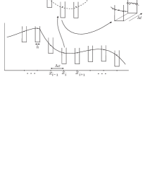
(a) The gap-tooth scheme

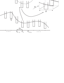
(b) Introduction of buffers

Figure 1: A schematic representation of the two variants of the gap-tooth scheme (with and without buffer boxes).

4 Results

We first show analytically and numerically that the standard gap-tooth scheme converges for equation (4). We then analyze convergence of the scheme with buffers and Dirichlet boundary conditions through its damping factors.

4.1 Convergence of the gap-tooth scheme

Theorem 1.

The gap-tooth scheme, applied to equation (4) with exact, analytical integration within the boxes, and boundary conditions defined through interpolating polynomials of (even) order $k$, is equivalent to a finite difference discretization of equation (4) of order $k$ central differences in space and an explicit Euler time step.

Proof.

When using exact (analytic) integration in each box, we can find an explicit formula for the gap-tooth time-stepper. The initial profile is given by (8), $\tilde{u}_{i}(x,t_{n})=a(x-x_{i})^{2}+b(x-x_{i})+c$. Due to the Neumann boundary conditions, time integration can be done analytically, using

$$\tilde{u}(x,t_{n}+\Delta t)=a(x-x_{i})^{2}+b(x-x_{i})+c+2a\cdot a^{*}\Delta t$$

Averaging this profile over the box gives the following time-stepper for the box averages,

$$U_{i}^{n}=U_{i}^{n}+a^{*}\frac{s^{+}_{i}-s^{-}_{i}}{h}\Delta t.$$

We know that $s^{\pm}_{i}=\left.\frac{\mathrm{d}}{\mathrm{d}x}p_{i}^{k}(x,t_{n})\right|_{x_{i}\pm\frac{h}{2}},$ where $p_{i}^{k}(x,t_{n})$ is determined by (5). One can easily verify that

$$\frac{\mathrm{d}^{2}}{\mathrm{d}x^{2}}\mathcal{S}_{h}(p_{i}^{k})(x,t_{n})=\frac{s^{+}_{i}-s^{-}_{i}}{h},$$

is a $k$-th order approximation of $\frac{\partial^{2}u}{\partial x^{2}}$, which concludes the proof.∎∎

As an example, we apply the gap-tooth scheme to the diffusion equation (4) with $a^{*}=1$. We choose an initial condition $U(x,t)=1-|2x-1|$, with Dirichlet boundary conditions, and show the result of a fourth-order gap-tooth simulation with $\Delta x=0.05$, $\Delta t=5\cdot 10^{-3}$ and $h=0.01$. Inside each box, we used a second order finite difference scheme with microscopic spatial mesh size $\delta x=1\cdot 10^{-3}$ and $\delta t=5\cdot 10^{-7}$. The results are shown in figure 2.

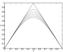
(a) Numerical solution

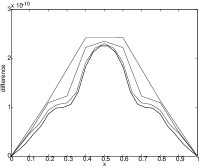
(b) Difference with FD

Figure 2: The gap-tooth scheme of fourth order for eq. (4) at $t=0,4\cdot 10^{-3},\ldots,2\cdot 10^{-2}$.

4.2 Damping factors

Convergence results are typically established by proving consistency and stability. If one can prove that the error in each time step can be made arbitrarily small by refining the spatial and temporal mesh size, and that an error made at time $t_{n}$ does not get amplified in future time-steps, one has proved convergence. This requires the solution operator to be stable as well.

In the abscense of explicit formulas, one can examine the damping factors of the time-stepper. If, for decreasing mesh sizes, all (finitely many) eigenvalues and eigenfunctions of the time-stepper converge to the dominant eigenvalues and eigenfunctions of the time evolution operator, one expects the solution of the scheme to converge to the true solution of the evolution problem.

Consider equation (4) with Dirichlet boundary conditions $u(0,t)=0$ and $u(1,t)$, and denote its solution at time $t$ by the time evolution operator

$$u(x,t)=s(u_{0}(x);t),$$ (11)

We know that

$$s(\sin(m\pi x);t)=\mathrm{e}^{-(m\pi)^{2}t}\sin(m\pi x),\qquad m\in\mathbb{N}.$$

Therefore, if we consider the time evolution operator over a fixed time $\bar{t}$, $s(\cdot,\bar{t})$, then this operator has eigenfunctions $\sin(m\pi x)$, with resp. eigenvalues

$$\lambda_{m}=\mathrm{e}^{-{(m\pi)}^{2}\bar{t}}.$$ (12)

A good (finite difference) scheme approximates well all eigenvalues whose eigenfunctions can be represented on the given mesh. We note that it is possible to decouple the time horizon $\bar{t}$ from the gap-tooth (or finite-difference) time-step $\Delta t$, in order to study the effect of different discretizations on the same reporting horizon.

Since the operator defined in (11) is linear, the numerical time integration is equivalent to a matrix-vector product. Therefore, we can compute the eigenvalues using matrix-free linear algebra techniques, even for the gap-tooth scheme, for which it might not even be possible to obtain a closed expression for the matrix. We note that this analysis gives us an indication about the quality of the scheme, but it is by no means a proof of convergence.

We illustrate this with the computation of the eigenvalues of the gap-tooth scheme with Neumann box boundary conditions. In this case, we know from theorem 1 that these eigenvalues should correspond to the eigenvalues of a finite difference scheme on the same mesh. We compare the eigenvalues of the gap-tooth scheme of order $k=2$ for equation (4) with diffusion coefficient $a^{*}=0.45825686$. As method parameters, we choose $\Delta x=0.05$, $h=5\cdot 10^{-3}$, $\Delta t=2.5\cdot 10^{-4}$ for a time horizon $\bar{t}=4\cdot 10^{-3}$, which corresponds to 16 gap-tooth steps. Inside each box, we use a finite difference scheme of order $2$ with $\delta x=1\cdot 10^{-4}$ and an implicit Euler time-step of $5\cdot 10^{-5}$. We compare these eigenvalues to those the finite difference scheme with $\Delta x=0.05$ and $\Delta t=2.5\cdot 10^{-4}$, and with the dominant eigenvalues of the “exact” solution (a finite difference approximation with $\Delta x=1\cdot 10^{-3}$ and $\Delta t=1\cdot 10^{-7}$). The result is shown in figure 3. The difference between the finite difference approximation and the gap-tooth scheme in the higher modes, which should be zero according to theorem 1, is due to the numerical solution inside each box and the use of numerical quadrature for the average.

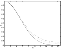
Figure 3: Comparison between the damping factors (left) and the eigenfunction corresponding to eigenvalue $\lambda_{3}$ (right) of the exact solution (full line), the finite difference approximation (dashed) and the gap-tooth scheme (dotted). The eigenfunction of the gap-tooth scheme is indistinguishable of the finite difference eigenfunction.

We now examine the effect of introducing a buffer region, as described in section 3.2. We consider again equation (4) with $a^{*}=0.45825686$, and we take the gap-tooth scheme with parameters $\Delta x=0.05$, $h=5\cdot 10^{-3}$, $\Delta t=2.5\cdot 10^{-4}$ for a time horizon $\bar{t}=4\cdot 10^{-3}$, and an internal time-stepper as above. We introduce a buffer region of size $H$, and we impose Dirichlet boundary conditions at the outer boundary of the buffer region. Lifting is done in identically the same way as for the gap-tooth scheme without buffers; we only use (9) as the initial condition in the larger box $[x_{i}-\frac{H}{2},x_{i}+\frac{H}{2}]$. We compare the eigenvalues again with the equivalent finite difference scheme and the exact solution, for increasing sizes of the buffer box $H$. Figure 4 shows that, as $H$ increases, the eigenvalues of the scheme converge to those of the original gap-tooth scheme. We see that, in this case, we would need a buffer of size $H=4\cdot 10^{-2}$, i.e. 80% of the original domain, for a good approximation of the damping factors. Note that it is conceptually possible, though inefficient, to let the buffer boxes overlap.

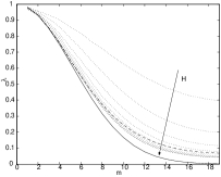
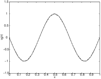
Figure 4: Comparison between the damping factors (left) and the eigenfunction corresponding to the eigenvalue $\lambda_{3}$ (right) of the exact solution (full line), the finite difference scheme (dashed) and the gap-tooth scheme with buffers (dash-dotted lines) for increasing buffer sizes $H=2\cdot 10^{-2},3\cdot 10^{-2}\ldots,1\cdot 10^{-1}$.

5 Summary/Conclusions

We described the gap-tooth scheme for the numerical simulation of multi-scale problems. This scheme simulates the macroscopic behaviour over a macroscopic domain when only a microscopic model is explicitly available. In the case of diffusion, we showed equivalence of our scheme to standard finite differences of arbitrary (even) order, both theoretically and numerically.

We showed that it is possible, even without analytic formulas, to study the properties of the gap-tooth scheme and generalizations through the damping factors of the resulting coarse time-$\Delta t$ map. We illustrated this for the original gap-tooth scheme and for an implementation using Dirichlet boundary conditions in a buffer box. We showed that, as long as the buffer region is “large enough” to shield the internal region from the boundary effects over a time $\Delta t$, we get a convergent scheme. Therefore, we are able to use microscopic codes in the gap-tooth scheme without modification.

In a forthcoming paper, we will explore, using these damping factors for many different types of boundary conditions, the relation between the quality of the boundary conditions, the size of the buffer region and the time-step before reinitialization. We will investigate the trade-off between the effort required to impose a particular type of boundary conditions (and the eventual macroscopically inspired control-based strategy) and the efficiency gain due to smaller buffer sizes and/or longer possible time-steps before reinitialization. Here, we showed that this investigation is made possible by studying the damping factors of the resulting coarse time-$\Delta t$ map.

Acknowledgements GS is a Research Assistant of the Fund of Scientific Research - Flanders. This work has been partially supported by an IUAP grant and by the Fund of Scientific Research through Research Project G.0130.03 (GS, DR), and by the AFOSR and the NSF (IGK). The authors thank Olof Runborg for discussions that improved this text and the organizers of the Summer School in Multi-scale Modeling and Simulation in Lugano.

References

- [EE03] W. E and B. Engquist. The heterogeneous multi-scale methods. Comm. Math. Sci., 1(1):87–132, 2003.
- [GK02] C.W. Gear and I.G. Kevrekidis. Boundary processing for Monte Carlo simulations in the gap-tooth scheme. physics/0211043 at arXiv.org, 2002.
- [GKT02] C.W. Gear, I.G. Kevrekidis, and C. Theodoropoulos. “Coarse” integration/bifurcation analysis via microscopic simulators: micro-Galerkin methods. Comp. Chem. Eng., 26(7-8):941–963,2002.
- [GLK03] C.W. Gear, J. Li, and I.G. Kevrekidis. The gap-tooth method in particle simulations. Physics Letters A, 316:190–195, 2003.
- [Had99] N. G. Hadjiconstantinou. Hybrid atomistic-continuum formulations and the moving contact-line problem. J. Comp. Phys., 154:245–265, 1999.
- [HW97] T.Y. Hou and X.H. Wu. A multiscale finite element method for elliptic problems in composite materials and porous media. J. Comp. Phys. , 134:169–189, 1997.
- [KGK02] I.G. Kevrekidis, C.W. Gear, J.M. Hyman, P.G. Kevrekidis, O. Runborg, and C. Theodoropoulos. Equation-free multiscale computation: enabling microscopic simulators to perform system-level tasks. Comm. Math. Sci. Submitted, physics/0209043 at arxiv.org, 2002.
- [LLY98] J. Li, D. Liao, S. Yip. Imposing field boundary conditions in MD simulation of fluids: optimal particle controller and buffer zone feedback, Mat. Res. Soc. Symp. Proc, 538(473-478), 1998.
- [SKR03] G. Samaey, I.G. Kevrekidis, and D. Roose. The gap-tooth scheme for homogenization problems. SIAM MMS, 2003. Submitted.
- [SGK03] S. Setayeshar, C.W. Gear, H.G. Othmer, and I.G. Kevrekidis. Application of coarse integration to bacterial chemotaxis. SIAM MMS. Submitted, physics/0308040 at arxiv.org, 2003.