Double-resonant extremely asymmetrical scattering of electromagnetic waves in periodic arrays separated by a gap

Abstract

Preprint of:

D. K. Gramotnev and T. A. Nieminen,

“Double-resonant extremely asymmetrical scattering of

electromagnetic waves in periodic arrays separated by a gap”,

Optical and Quantum Electronics 33, 1–17 (2001)

Two strong simultaneous resonances of scattering—double-resonant extremely asymmetrical scattering (DEAS)—are predicted in two parallel, oblique, periodic Bragg arrays separated by a gap, when the scattered wave propagates parallel to the arrays. One of these resonances is with respect to frequency (which is common to all types of Bragg scattering), and another is with respect to phase variation between the arrays. The diffractional divergence of the scattered wave is shown to be the main physical reason for DEAS in the considered structure. Although the arrays are separated, they are shown to interact by means of the diffractional divergence of the scattered wave across the gap from one array into the other. It is also shown that increasing separation between the two arrays results in a broader and weaker resonance with respect to phase shift. The analysis is based on a recently developed new approach allowing for the diffractional divergence of the scattered wave inside and outside the arrays. Physical interpretations of the predicted features of DEAS in separated arrays are also presented. Applicability conditions for the developed theory are derived.

I Introduction

Extremely asymmetrical scattering (EAS) occurs when the scattered wave propagates parallel to the front boundary of a strip-like periodic Bragg array kishino1971 ; kishino1972 ; bedynska1973 ; bedynska1974 ; bakhturin1995 ; gramotnev1995 ; gramotnev1996 ; gramotnev1997 ; gramotnev1999a ; gramotnev1999b ; gramotnev1999c . Steady-state EAS is characterized by a strong resonant increase of the scattered wave amplitudes inside and outside the array. The smaller the grating amplitude, the larger the amplitudes of the scattered waves kishino1972 ; bakhturin1995 ; gramotnev1995 ; gramotnev1996 ; gramotnev1997 ; gramotnev1999a ; gramotnev1999b ; gramotnev1999c . In addition, the incident and scattered waves inside the array split into three waves each bakhturin1995 ; gramotnev1995 ; gramotnev1996 ; gramotnev1997 ; gramotnev1999a ; gramotnev1999b ; gramotnev1999c . Two of these scattered waves and two of the incident waves inside the array are evanescent waves localized near the array boundaries bakhturin1995 ; gramotnev1995 ; gramotnev1996 ; gramotnev1997 . The third scattered wave is a plane wave propagating at a grazing angle into the array bakhturin1995 ; gramotnev1995 ; gramotnev1996 ; gramotnev1997 . All these features demonstrate that EAS is radically different from the conventional Bragg scattering in periodic arrays.

There are two opposing physical mechanisms affecting scattering in the extremely asymmetric geometry bakhturin1995 ; gramotnev1995 ; gramotnev1996 ; gramotnev1997 ; gramotnev1999a ; gramotnev1999b ; gramotnev1999c . On the one hand, the scattered wave amplitude must increase along the direction of its propagation (parallel to the front boundary of the periodic array) due to scattering of the incident wave inside the array. On the other hand, the scattered wave amplitude must decrease along the direction of its propagation due to the diffractional divergence of this wave bakhturin1995 ; gramotnev1995 ; gramotnev1996 ; gramotnev1997 ; gramotnev1999a ; gramotnev1999b ; gramotnev1999c . This diffractional divergence was demonstrated to be the main physical reason for EAS. In the steady-state case of scattering in the geometry of EAS, the contributions to the scattered wave amplitude from the two opposing mechanisms must exactly compensate each other. A new powerful approach for a simple theoretical analysis of EAS, based on allowance for the diffractional divergence of the scattered wave, was introduced and justified bakhturin1995 ; gramotnev1995 ; gramotnev1996 ; gramotnev1997 ; gramotnev1999a ; gramotnev1999b ; gramotnev1999c .

It was demonstrated that in non-uniform arrays with varying phase of the grating, EAS is characterized by two simultaneous resonances—one with respect to frequency, and the other with respect to the phase variation in the grating gramotnev1999a ; gramotnev1999c ; gramotnev2000 . As a result, typical scattered wave amplitudes in this case appear to be many times larger than those for EAS in uniform arrays. This effect was called double-resonant extremely asymmetrical scattering (DEAS) gramotnev1999a ; gramotnev1999c ; gramotnev2000 . DEAS was described for a non-uniform array that consists of two joint strip-like periodic arrays with different phases of the grating, i.e. a step-like variation of the grating phase occurs at the interface between the arrays gramotnev1999a ; gramotnev1999c ; gramotnev2000 .

The main physical reason for DEAS is related to the diffractional divergence of the scattered wave from one of the joint periodic arrays into another. For example, the scattered wave from the second array, propagating parallel to the array boundaries, diverges into the first array, and is re-scattered by the grating in the first array. Due to the phase difference between the arrays (that should be close to $\pi$), the resultant re-scattered wave appears to be approximately in phase with the incident wave inside the first array. Therefore, the amplitude of the incident wave (that is analogous to a force driving resonant oscillations) is increased due to the constructive interference with the mentioned re-scattered wave. The same speculations are valid for the second array. This is the reason for a substantial resonant increase in the scattered wave amplitude in DEAS compared to EAS gramotnev1999a ; gramotnev1999c ; gramotnev2000 .

It was also demonstrated that strong DEAS (i.e. strong resonance with respect to phase variation between the arrays) can take place only if the array width is smaller than a critical width. Physically, half of this critical width is equal to a distance through which the scattered wave can be spread inside the array due to the diffractional divergence before being re-scattered in the grating gramotnev1999a ; gramotnev1999c ; gramotnev2000 . It is obvious that only within this distance from the interface between the two joint arrays can the diffractional divergence significantly affect scattering.

The aim of this paper is to demonstrate that strong DEAS can take place not only in two joint periodic arrays, but also in two oblique, strip-like, periodic arrays separated by a gap. We will show that separated arrays can interact with each other by means of the diffractional divergence of the scattered waves across the gap. This interaction will be demonstrated to decrease with increasing gap width. The effect of gap width on the incident and scattered wave amplitudes inside and outside the arrays will be investigated. Steady-state DEAS of bulk and guided optical waves will be analyzed. Applicability conditions for the developed approximate theory will be determined and investigated.

II Coupled wave equations

In this section we present coupled wave equations and their solutions in the case of DEAS of bulk TE electromagnetic waves in two separated uniform periodic arrays (Fig. 1) that are represented by small sinusoidal variations of the mean dielectric permittivity:

$$\begin{array}[]{l}\epsilon_{s}=\epsilon+\epsilon_{1}\exp(\mathrm{i}\mathbf{q}\cdot\mathbf{r})+\epsilon_{1}^{\ast}\exp(-\mathrm{i}\mathbf{q}\cdot\mathbf{r}),\\ \epsilon_{s}=\epsilon+\epsilon_{2}\exp(\mathrm{i}\mathbf{q}\cdot\mathbf{r})+\epsilon_{2}^{\ast}\exp(-\mathrm{i}\mathbf{q}\cdot\mathbf{r}),\\ \\ \epsilon_{s}=\epsilon,\end{array}\begin{array}[]{l}\textrm{if}\;\;0<x<L_{1};\\ \textrm{if}\;\;L+L_{1}<x\\ <L+L_{1}+L_{2};\\ \textrm{otherwise,}\end{array}$$ (1)

where $L_{1}$ and $L_{2}$ are the widths of the first and second arrays (Fig. 1), $L$ is the width of the gap between the arrays, $\mathbf{q}$ is the reciprocal lattice vector, $|\mathbf{q}|=2\pi/\Lambda$, $\Lambda$ is the grating period that is the same in both the arrays, the mean dielectric permittivity $\epsilon$ is the same in all parts of the structure (inside and outside the arrays), and the amplitudes of the gratings $\epsilon_{1}$ and $\epsilon_{2}$ in the first and the second arrays are assumed to be small:

$$|\epsilon_{1,2}|/\epsilon\ll 1.$$ (2)

The grating amplitudes $\epsilon_{1}$ and $\epsilon_{2}$ can differ in magnitude and/or in phase. There is no dissipation of electromagnetic waves inside or outside the array, i.e. $\epsilon$ is real and positive.

Figure 1: The geometry of DEAS in two non-uniform strip-like periodic Bragg arrays of width $L_{1}$ and $L_{2}$, separated by a gap of width $L$.

A plane TE electromagnetic wave (with the electric field parallel to the $z$-axis) is incident onto the first array at an angle $\theta_{0}$ (measured from the $x$-axis counter-clockwise—Fig. 1). We assume that the Bragg condition is satisfied precisely:

$$\mathbf{k}_{1}-\mathbf{k}_{0}=-p\mathbf{q},$$ (3)

where $p$ takes one of the values: $\pm 1,\pm 2,...$, $\mathbf{k}_{0}$ is the wave vector of the incident wave, $\mathbf{k}_{1}$ is parallel to the array boundaries (Fig. 1), $|\mathbf{k}_{1}|=|\mathbf{k}_{0}|=k_{0}=\omega\epsilon^{1/2}/c$, $\omega$ is the angular frequency, and $c$ is the speed of light in vacuum.

As has been demonstrated previously bakhturin1995 ; gramotnev1995 ; gramotnev1996 ; gramotnev1997 ; gramotnev1999a ; gramotnev1999b ; gramotnev1999c ; gramotnev2000 , strong resonant increase in the scattered wave amplitude in the extremely asymmetrical geometry can only occur for small grating amplitudes—see condition (2). In this case, the two wave approximation kogelnik1969 is valid, and only two harmonics in the Floquet expansion—incident and scattered waves—need to be taken into account inside and outside the array:

$$E(x) = E_{0}(x)\exp\left\{\mathrm{i}k_{0x}x+\mathrm{i}k_{0y}y-\mathrm{i}\omega t\right\}$$ (4)

$$+E_{1}(x)\exp\left\{\mathrm{i}k_{0}y-\mathrm{i}\omega t\right\},$$

where $E_{0}(x)$ and $E_{1}(x)$ are the varying amplitudes of the electric fields in the incident and scattered waves, respectively, $k_{0x}=k_{0}\cos\theta_{0}$, and $k_{0y}=k_{0}\sin\theta_{0}$. Detailed discussions of applicability conditions for this approximation in the cases of EAS and DEAS are presented below in Section 4.

Similarly to how it was done in bakhturin1995 ; gramotnev1996 ; gramotnev2000 ; gramotnev1999a ; gramotnev1999c , the coupled wave equations in the separated arrays, describing DEAS, can be derived by means of separate analyses of the diffractional divergence of the scattered wave (by means of the parabolic equation of diffraction bakhturin1995 ; gramotnev1999a ; gramotnev1999c ; gramotnev2000 or Fourier analysis gramotnev1996 ; gramotnev2000 ), and scattering (by means of the conventional theory of scattering kogelnik1969 ; gramotnev1996 ; stegeman1981 ; popov1985 ; wellerbrophy1988 ; hall1990 ). In the steady-state DEAS the contribution to the scattered wave amplitude from scattering is exactly compensated by the contribution from the diffractional divergence. In the same fashion as in gramotnev1996 ; gramotnev2000 ; gramotnev1999c , the comparison of these contributions leads to the coupled wave equations in the separated arrays:

$$\frac{\mathrm{d}}{\mathrm{d}x}E_{0}(x)=\left\{\begin{array}[]{l}\mathrm{i}K_{11}E_{1}(x)\\ 0\\ \mathrm{i}K_{12}E_{1}(x)\\ {}\end{array}\begin{array}[]{l}\textrm{if}\;\;0\leq x\leq L_{1},\\ \textrm{if}\;\;L_{1}<x<L+L_{1},\\ \textrm{if}\;\;L+L_{1}\leq x\\ \leq L+L_{1}+L_{2},\end{array}\right.$$ (5)

$$\frac{\mathrm{d}^{2}}{\mathrm{d}x^{2}}E_{1}(x)=\left\{\begin{array}[]{l}\mathrm{i}-K_{01}E_{0}(x)\\ 0\\ \mathrm{i}K_{02}E_{0}(x)\\ {}\end{array}\begin{array}[]{l}\textrm{if}\;\;0\leq x\leq L_{1},\\ \textrm{if}\;\;L_{1}<x<L+L_{1},\\ \textrm{if}\;\;L+L_{1}\leq x\\ \leq L+L_{1}+L_{2},\end{array}\right.$$ (6)

where

$$K_{1j}=\Gamma_{1j}\cos\eta/\cos\theta_{0},$$ (7)

$$K_{0j}=-2k_{1}\Gamma_{0j}\sin(\eta-\theta_{0}),$$ (8)

indices $j=1,2$ correspond to the first and second arrays, respectively, $\eta$ is the angle between the direction of propagation of the incident wave and the $x_{0}$-axis (Fig. 1), $\Gamma_{0j}$ and $\Gamma_{1j}$ are the coupling coefficients in the well-known coupled wave equations kogelnik1969 ; stegeman1981 ; popov1985 ; wellerbrophy1988 ; hall1990 ; gramotnev1996

$$\mathrm{d}E_{0}/\mathrm{d}x_{0}=\mathrm{i}\Gamma_{1j}E_{1},\;\;\;\mathrm{d}E_{1}/\mathrm{d}x_{0}=\mathrm{i}\Gamma_{0j}E_{0}$$ (9)

for the conventional dynamic theory of scattering in two isolated uniform arrays with the grating fringes parallel to the array boundaries, and with the grating amplitudes $\epsilon_{1}$ (for $j=1$) and $\epsilon_{2}$ (for $j=2$).

Note that Equations (5)–(9) are directly applicable for the description of DEAS of all types of waves, including optical modes guided by a slab with a periodically corrugated boundary. In this case, the plane of Fig. 1 is the plane of a guiding slab, and the incident and scattered waves are modes guided by this slab. The only difference between scattering of different types of waves are different values of coupling coefficients $\Gamma_{0j}$ and $\Gamma_{1j}$ that are already determined in the conventional theory of scattering kogelnik1969 ; stegeman1981 ; popov1985 ; wellerbrophy1988 ; hall1990 ; gramotnev1996 . For example, in the case of bulk TE electromagnetic waves in arrays described by Equation (1) we obtain kogelnik1969 ; gramotnev1996 :

$$\Gamma_{0j}=-\Gamma_{1j}^{\ast}=-\epsilon_{j}^{\ast}\omega^{2}/[2c^{2}k_{0}\cos\eta].$$ (10)

We have also used $k_{1}$ instead of $k_{0}$ in Equation (8), because for guided optical modes $k_{1}$ may not be equal to $k_{0}$ (e.g., for scattering of TE modes guided by a slab into TM modes of the same slab).

The solutions to coupled wave equations (5) and (6) inside the first ($j=1$) and the second ($j=2$) arrays can be written as bakhturin1995 ; gramotnev1996 ; gramotnev1999b ; gramotnev2000 :

$$E_{1}(x) = C_{1j}\exp(\mathrm{i}\lambda_{1j}x)+C_{2j}\exp(\mathrm{i}\lambda_{2j}x)$$

$$+C_{3j}\exp(\mathrm{i}\lambda_{3j}x),$$

$$E_{0}(x) = D_{1j}\exp(\mathrm{i}\lambda_{1j}x)+D_{2j}\exp(\mathrm{i}\lambda_{2j}x)$$

$$+D_{3j}\exp(\mathrm{i}\lambda_{3j}x),$$

where $\lambda_{1j}=\gamma_{j}$, $\lambda_{2j}=-(1-\mathrm{i}3^{1/2})\gamma_{j}/2$, $\lambda_{2j}=-(1+\mathrm{i}3^{1/2})\gamma_{j}/2$, and

$$\gamma_{j}=[K_{0j}K_{1j}]^{1/3}.$$ (12)

In front of and behind the arrays,

$$\begin{array}[]{l}E_{1}(x)=A_{1},\\ E_{1}(x)=A_{3},\end{array}\begin{array}[]{l}E_{0}(x)=E_{00},\\ E_{0}(x)=E_{01},\end{array}\begin{array}[]{l}\textrm{if}\;\;x<0;\\ \textrm{if}\;\;x>L+L_{1}+L_{2}.\end{array}$$ (13)

In the gap between the arrays (i.e. for $L_{1}<x<L+L_{1}$) Equations (5) and (6) yield:

$$E_{1}(x)=A_{21}+A_{22}x,E_{0}(x)=B.$$ (14)

These equations suggest that, although there is no scattering in the gap between the arrays, the scattered wave amplitude is not constant due to the interaction between the scattered waves diverging from each of the two arrays.

A relationship between the amplitudes of the incident and scattered waves inside the array $C_{ij}$ and $D_{ij}$ ($j=1,2$; $i=1,2,3$) can be established by substituting Equations (11) into Equations (6):

$$C_{ij}=\lambda_{ij}D_{ij}/K_{1}$$ (15)

The remaining unknown constants $A_{1}$, $A_{3}$, $A_{21}$, $A_{22}$, $B$, $E_{01}$, and $D_{ij}$ can be determined from the boundary conditions gramotnev1999a ; gramotnev1999c of continuity of the fields and their derivatives across the four array boundaries (note however, that in the considered two-wave approximation, the derivatives of the fields in the incident wave are not continuous across the boundaries gramotnev1996 ; gramotnev1997 ; gramotnev1999a ; gramotnev1999b ; gramotnev1999c ; gramotnev2000 . The resultant analytical equations for these constants (amplitudes) appear to be too awkward to be presented here. Instead, in the next section we analyze these solutions numerically for different gap widths and array parameters.

III Analysis of DEAS in separated arrays

As expected, the form of solutions (11)–(13) is the same as for two joint uniform arrays gramotnev1999a ; gramotnev2000 . However, due to the presence of the gap with the field given by Equation (14), the overall pattern of scattering changes substantially. That is, the particular dependencies of the incident and scattered wave amplitudes $E_{1}(x)$ and $E_{0}(x)$ inside and outside the arrays are noticeably different from those obtained for EAS and DEAS in uniform and non-uniform arrays without the gap gramotnev1999a ; gramotnev1999b ; gramotnev1999c ; gramotnev2000 . This will be seen from the figures below.

Equations (11)–(15) are also written in such a way that they are valid for any types of waves, including guided TE and TM modes in a slab with a corrugated interface. The boundary conditions at the array boundaries will also be the same for all types of waves, because actually there are no physical boundaries since the mean parameters of the media are the same inside and outside the array. Therefore, we can consider bulk TE electromagnetic waves in arrays described by Equation (1), keeping in mind that all the results below are valid, for example, for DEAS of guided optical modes gramotnev1999a ; gramotnev1999c ; gramotnev2000 .

Figure 2: The dependencies of relative (normalized) amplitudes of the scattered wave at the front array boundary on phase shift $\phi$ between the arrays for different values of gap width $L$: (a) $L=0$, (b) $L=3$ µm, (c) $L=6$ µm, (d) $L=9$ µm, and (e) $L=+\infty$. Scattering of bulk TE electromagnetic waves takes place in the structure with $\epsilon=5$, $\epsilon_{1}=|\epsilon_{2}|=5\times 10^{-3}$, $\epsilon_{2}=\epsilon_{1}\exp(\mathrm{i}\phi)$, $\theta_{0}=\pi/4$, $L_{1}=L_{2}=15$ µm, $\lambda_{\mathrm{vacuum}}=1$ µm, the grating period $\Lambda\approx 0.58$ µm, $\eta=3\pi/8$.

Fig. 2 presents typical dependencies of the relative scattered wave amplitude at the front boundary of the first array (i.e. at $x=0$) on the phase variation $\phi$ between the arrays for different values of the gap width $L$. The structural parameters are as follows: $\epsilon=5$, $\epsilon_{1}=|\epsilon_{2}|=5\times 10^{-3}$, $\epsilon_{2}=\epsilon_{1}\exp(\mathrm{i}\phi)$, $\theta_{0}=\pi/4$, $L_{1}=L_{2}=15$ µm, i.e. the two separated arrays, apart from a phase difference $\phi$ between them, are identical. The period of the structure $\Lambda$ is also the same for both the arrays, and is unambiguously determined by the Bragg condition (3) and the angle of incidence $\theta_{0}$: $\Lambda\approx 0.58$ µm, and $\eta=3\pi/8$. The wavelength in vacuum is $\lambda=1$ µm.

Fig. 2 demonstrates that as the gap width decreases, the maximum of the scattered wave amplitude at an optimal (resonant) value of $\phi$ becomes sharper and stronger until the gap width reaches zero (curve (a)). It can be seen that even if the arrays are separated, they can effectively interact across the gap, which results in DEAS. Since the scattered waves in both the arrays propagate parallel to the array boundaries (Fig. 1), the interaction (interference) between the waves can only occur due to their diffractional divergence from one array into another across the gap. This clearly demonstrates not only a new interesting effect in periodic arrays in the extremely asymmetrical geometry, but also most explicitly confirms the unique role of the diffractional divergence in DEAS.

Curves (b)–(d) in Fig. 2 show the transition from DEAS in the joint arrays (curve (a)) to EAS in the uniform array of $L_{1}=15$ µm (curve (e)) as the gap width increases from zero to infinity. Even small gap widths, e.g., $L=3$ µm (curve (b) in Fig. 2), which is about seven wavelengths in the structure, result in a noticeable decrease of the scattered wave amplitude compared to DEAS in the joint arrays. This is because the effectiveness of the diffractional divergence in spreading the scattered wave across the gap quickly decreases with increasing gap width.

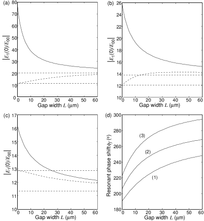
Figure 3: Solid and dashed curves in (a)–(c) present the dependencies of relative scattered wave amplitudes at the front boundary $x=0$ on gap width $L$ for bulk TE electromagnetic waves in the structure with $\epsilon=5$, $\epsilon_{1}=|\epsilon_{2}|=5\times 10^{-3}$, $\epsilon_{2}=\epsilon_{1}\exp(\mathrm{i}\phi)$, $\theta_{0}=\pi/4$, $\lambda_{\mathrm{vacuum}}=1$ µm, $\phi=\phi_{rf}$ (solid curves), and $\phi=0$ (dashed curves); (a) $L_{1}=L_{2}=10$ µm; (b) $L_{1}=L_{2}=15$ µm; (c) $L_{1}=L_{2}=20$ µm. Dotted lines: $L=+\infty$ (i.e., uniform isolated arrays of widths $L_{1}$); dash-and-dot lines: $L=0$ and $\phi=0$ (i.e., uniform isolated arrays of widths $2L_{1}$). Resonant values $\phi_{rf}$ of the phase shift between the arrays (i.e., the values of $\phi$ at which the scattered wave amplitude is maximal at the front boundary $x=0$) are presented in (d) as functions of gap width $L$: (1) $L_{1}=L_{2}=10$ µm; (2) $L_{1}=L_{2}=15$ µm; (3) $L_{1}=L_{2}=20$ µm.

The dependencies of maximal scattered wave amplitudes at the front array boundary (i.e. at $x=0$) on gap width $L$ in the case of DEAS are presented by the solid curves in Fig. 3a–c for different array widths: (a) $L_{1}=L_{2}=10$ µm, (b) $L_{1}=L_{2}=15$ µm, (c) $L_{1}=L_{2}=20$ µm. Fig. 3d presents the resonant phase shifts $\phi_{rf}$ between the arrays as functions of gap width $L$ for the same array widths: 10 µm (curve 1), 15 µm (curve 2), and 20 µm (curve 3). In other words, each value of $|E_{1}(0)/E_{00}|$ given by the solid curves in Fig. 3a–c has been determined at the corresponding resonant value of the phase shift $\phi=\phi_{rf}$ given by Fig. 3d. The index $f$ in $\phi_{rf}$ indicates that this is the value of the phase shift at which the scattered wave amplitude is maximal at the front boundary $x=0$. Dotted lines in Fig. 3a–c correspond to EAS in the first of the uniform arrays in the absence of the second array. Obviously, these lines must also correspond to the case when the gap is infinitely large. Therefore, if the gap width increases to infinity, the solid curves in Fig. 3a–c tend to the dotted lines. The dashed curves in Fig. 3a–c present the amplitudes of the scattered wave at the front boundary of the first array as functions of gap width $L$ for zero phase shift $\phi=0$ (i.e. for EAS in separated arrays). In this case, the interaction between the arrays does not result in a significant increase in the scattered wave amplitude compared to EAS in the first uniform array (the dotted lines). The amplitude of the scattered wave at the front boundary of the first array basically varies from its value for a uniform array of the width $2L_{1}$ (dash-and-dot lines in Fig. 3a–c) to the value for the first isolated uniform array (dashed curves in Fig. 3a–c). This clearly demonstrates strong differences between DEAS and EAS in separated arrays. The existence of a phase shift between the arrays, which is close to the resonant value (Fig. 3d), results in a substantial resonant increase in the scattered wave amplitude (solid curves in Fig. 3a–c).

The dependencies of the amplitudes of the incident and scattered waves on the $x$-coordinate inside and between the arrays is presented in Fig. 4 for resonant values of $\phi=\phi_{r}$, where $\phi_{r}$ corresponds to maximal scattered wave amplitudes in the middle of the gap ($\phi_{r}$ is very close to, but not equal to $\phi_{rf}$). It can be seen that the amplitude of the incident wave in the gap is constant, which is expected since there is no scattering in the gap, and the diffractional divergence of the incident wave is negligible (curves 2 and 3 in Fig. 4a, b). A maximum of the incident wave amplitude is achieved in the gap. However, this maximum quickly decreases with increasing gap width $L$ (Fig. 4a, b), reaching $E_{00}$ (the amplitude of the incident wave at the front boundary $x=0$) when the gap width is infinite—see curves 4 in Fig. 4a, b).

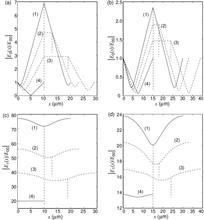
Figure 4: Typical dependencies of relative amplitudes of the incident [(a) and (b)] and scattered [(c) and (d)] waves on distance $x$ from the front boundary $x=0$ for narrow ($L_{1}=L_{2}<L_{c}$) arrays for different widths of the gap and arrays: (a) and (c): $L_{1}=L_{2}=10$ µm, $L=0$ and $\phi=\phi_{r}\approx 190.3$° (curves 1); $L=3$ µm and $\phi=\phi_{r}\approx 197.2$° (curves 2); $L=9$ µm and $\phi=\phi_{r}\approx 206.6$° (curves 3); $L=+\infty$ (curves 4). (b) and (d): $L_{1}=L_{2}=15$ µm, $L=0$ and $\phi=\phi_{r}\approx 197.6$° (curves 1); $L=3$ µm and $\phi=\phi_{r}\approx 200.9$° (curves 2); $L=9$ µm and $\phi=\phi_{r}\approx 199.3$° (curves 3); $L=+\infty$ (curves 4). $\phi_{r}$ is the value of $\phi$ at which the scattered wave amplitude is maximal in the middle of the gap (note that in general $\phi_{r}\neq\phi_{rf}$). All other structural parameters are the same as for Figs. 3 and 4: $\epsilon=5$, $\epsilon_{1}=|\epsilon_{2}|=5\times 10^{-3}$, $\epsilon_{2}=\epsilon_{1}\exp(\mathrm{i}\phi)$, $\theta_{0}=\pi/4$, $\lambda_{\mathrm{vacuum}}=1$ µm. The edges of the gap between the arrays are marked by the vertical dotted lines.

Fig. 4c, d demonstrate how the increase in the gap width from zero to infinity results in the transformation of the $x$ dependencies of the scattered wave amplitudes which are typical for DEAS in the joint arrays (curves 1 in Fig. 4c, d), into the $x$ dependencies of the scattered wave amplitudes which are typical for EAS in the uniform arrays (curves 4 in Fig. 4c, d).

Note that all the curves in Figs. 4a–d are shown only within the region $0<x<2L_{1}+L$ (recall that in our examples $L_{1}=L_{2}$). Outside this region, the relative (normalized) magnitude of the incident wave amplitude is equal to one (this is the consequence of energy conservation), and the amplitudes of the scattered waves are the same as at the array boundaries $x=0$ and $x=2L_{1}+L$ (i.e. constant).

It can be seen that DEAS can be strong only if the array widths $L_{1}$ and $L_{2}$ (in our examples, $L_{1}=L_{2}$) are less than the critical width $L_{c}$ that has been determined in our previous publications gramotnev1999b ; gramotnev2000 :

$$L_{c}\approx 2\left\{(\mathrm{e}k_{1})^{-1}|(E_{1})_{x=L_{1}}[\Gamma_{01}E_{00}\sin(\eta-\theta_{0})]^{-1}|\right\}^{1/2}$$ (16)

(recall that in the considered examples we have assumed that $\epsilon_{1}=|\epsilon_{2}|$, i.e. $|\Gamma_{01}|=|\Gamma_{02}|$, and the critical widths for the first and the second arrays are equal: $L_{c}=L_{c1}=L_{c2}$). In Equation (16), $(E_{1})_{x=L_{1}}$ is the maximal amplitude of the scattered wave at the interface between the two joint arrays in the limit of large array widths (i.e. when $L_{1}>L_{c}$) gramotnev2000 , and $\mathrm{e}=2.718$.

Physically, $L_{c}$ is the distance through which the diffractional divergence can spread the scattered wave along the $x$-axis inside the array before this wave is re-scattered by the grating gramotnev1999b ; gramotnev2000 . In our previous examples, Equation (16) gives $L_{c}\approx 15$ µm. If the width of the arrays $L_{1}=L_{2}<L_{c}$ (e.g., $L_{1}=10$ µm—Fig. 4a, c), then for the zero gap width the diffractional divergence effectively spreads the scattered wave from the second array throughout the first array, and vice versa. The interaction between the diffracted waves in both the arrays results in strong DEAS, i.e. in a resonant increase in the scattered wave amplitude at a resonant phase shift between the arrays (which should be relatively close to 180°)—see gramotnev1999a ; gramotnev1999b ; gramotnev2000 and curve 1 in Fig. 4c. In this case, the incident wave amplitude, after an insignificant decrease near the front boundary, strongly increases, reaching its maximum at the interface between the arrays—see gramotnev2000 and curve 1 in Fig. 4a. The detailed physical explanation of this effect has been presented in gramotnev2000 . The scattered wave with a very large amplitude (typical for the case with $L_{1}<L_{c}$—see curve 1 in Fig. 4c) results in a strong re-scattered wave that within a very short distance from the front boundary $x=0$ appears to be dominating the original incident wave inside the first array. The amplitude of this re-scattered wave quickly increases with distance into the first array—curve 1 in Fig. 4a. The small minimum of curve 1 near the front boundary $x=0$ is related to scattering of the incident wave (and thus reducing its amplitude) before the amplitude of the re-scattered wave becomes dominant (Fig. 4a). Thus, in the first array, the energy basically flows from the scattered wave into the incident wave, resulting in a substantial increase in the incident wave amplitude inside the array. The phase shift between the arrays (that should be relatively close to 180°) results in reversing the situation in the second array. That is, the energy of the powerful (at the interface $x=L_{1}$) incident wave starts flowing back into the scattered wave, resulting in the quick reduction of the incident wave amplitude back to its vale at the front boundary $x=0$ (see gramotnev2000 and curve 1 in Fig. 4a).

If there is a gap between the arrays, then the diffractional divergence becomes less effective in spreading the scattered wave from one array into another. This is because the typical gradient of the scattered wave amplitude across the gap (i.e. across the wave front) decreases with increasing gap width. Therefore the divergence of the scattered wave from one array into another becomes weaker. As a result, less effective interaction of the separated arrays takes place, and the resonant increase of the scattered wave amplitude becomes smaller (Figs. 2–3). In addition to this, the minima near the front ($x=0$) and rear ($x=2L_{1}+L$) boundaries of the structure become more pronounced with increasing $L$ (Fig. 4a). This is related to the reduction of the scattered wave amplitude inside the arrays (Fig. 4c), which results in the reduction of amplitude of the re-scattered wave. Thus the distance from the front boundary, within which the re-scattered wave becomes dominant over the incident wave, must increase, i.e. the minimum of the incident wave near the front boundary must shift towards the middle of the first array—Fig. 4a. On the left-hand side of this minimum the energy flows from the incident wave into the scattered wave, and on the other side, in the opposite direction (up to the rear boundary of the first array). If $L\neq+\infty$, the overall energy flow in the first array will still be from the scattered wave into the incident wave (similarly to DEAS in two joint arrays gramotnev2000 ). This results in larger amplitudes of the incident wave in the gap compared to its amplitude at the front boundary $x=0$ (Fig. 4a, b). At the same time, if $L\rightarrow+\infty$, then the amplitude of the incident wave in the gap becomes the same as at the front boundary. In this case the minimum of the incident wave amplitude appears to be in the middle of the first array (Fig. 4a), resulting in overall zero energy flow from the scattered wave into the incident wave.

This pattern of scattering is typical when $L_{1}\leq L_{c}$—see Fig. 4a–d. If the array width $L_{1}>L_{c}$, then the pattern of scattering is different, and is only weakly dependent on width of the gap between the arrays (Fig. 5a, b). Moreover, in this case, variations of the scattered and incident wave amplitudes, caused by varying gap width, are noticeable only within the regions of width $\approx L_{c}$ (in our example, Equation (16) gives $L_{c}\approx 15$ µm) in each of the arrays next to the gap (Fig. 5a, b). This is quite expected, since $L_{c}$ is the distance within which the scattered wave can be spread inside the array(s) due to the diffractional divergence, before being re-scattered by the grating gramotnev1999a ; gramotnev1999b ; gramotnev1999c ; gramotnev2000 .

Figure 5: Typical dependencies of relative amplitudes of the incident (a) and scattered (b) waves on distance $x$ from the front boundary $x=0$ for wide arrays with $L_{1}=L_{2}=40$ µm $>L_{c}\approx 15$ µm, and for different gap widths: $L=0$ and $\phi=\phi_{r}\approx 158.6$° (curves 1), $L=3$ µm and $\phi=\phi_{r}\approx 153.4$° (curves 2), $L=+\infty$ (curves 3). The other structural parameters are the same as for Fig. 4. The edges of the gap between the arrays are marked by the vertical dotted lines.

IV Applicability conditions of the theory

Applicability conditions for the two-wave approximation and for the new approach based on allowance for the diffractional divergence of the scattered wave are discussed in gramotnev2000 ; nieminen2000 . In particular, it has been shown that the applicability condition derived in moharam1978 ; moharam1980 ; moharam1985 appears to be insufficient for the case of EAS, and more restrictive inequalities should be used:

$$\begin{array}[]{l}4(\lambda_{\mathrm{m}}/L_{1})^{2}\ll\\ 4(\lambda_{\mathrm{m}}/L_{c})^{2}\ll\end{array}\begin{array}[]{l}\textrm{if}\;\;L_{1}\leq L_{c},\\ \textrm{if}\;\;L_{1}>L_{c},\end{array}$$ (17)

where $\lambda_{\mathrm{m}}$ is the wavelength in the medium, and $L_{c}$ is the critical width—see Equation (16).

Use of the two wave approximation (which in the case of strong EAS or DEAS is basically reduced to neglecting boundary scattering gramotnev2000 will result in a relative error that is of the order of the left-hand sides of inequalities (17).

Conditions (17) are written for the case of EAS in an isolated uniform array of width $L_{1}$ (i.e. for $L=+\infty$ in Fig. 1). For DEAS, the amplitudes of the scattered wave inside and outside the array can be significantly larger than for EAS gramotnev1999a ; gramotnev1999b ; gramotnev1999c , and there are four boundaries at which the edge effects can occur (Fig. 1). However, if $L=0$ and $L_{1}<L_{c}$, then the two waves due to boundary scattering from the joint interfaces of the two arrays will obviously be in antiphase with each other (since the phase shift between the arrays is about 180°). The scattered waves due to boundary scattering from the boundaries $x=0$ and $x=2L_{1}+L$ will also interfere destructively. Therefore, the edge effects will mainly result in an energy flow from the second array to the first array, while the overall energy flow from the structure will be approximately zero. Since the arrays are narrower than the critical width $L_{c}$, the energy flow between the arrays will be (at least partly) compensated by the diffractional divergence of the scattered wave.

If there is a gap of width $L\neq 0$ between the arrays, the situation becomes more complicated, because the waves resulting from boundary scattering may interfere constructively (depending on gap with $L$). This may result in a significant energy flow from the structure. Nevertheless, this energy flow is of the order of the energy flow between the arrays across the gap.

These speculations show that the approximate theory of DEAS is valid if the energy flow between the arrays (joint or separated), caused by boundary scattering, is negligible compared to the energy flow in the incident wave. Therefore, in accordance with gramotnev2000 , the condition we are looking for can be obtained by the multiplication of the left-hand side of Equation (17a) by the square of the ratio of the scattered wave amplitude typical for DEAS, $E_{1}$, to the scattered wave amplitude typical for EAS, i.e. $(E_{1})_{L=+\infty}$:

$$\frac{4\lambda_{\mathrm{m}}^{2}}{L_{1}^{2}}|(E_{1})_{L=+\infty}|^{2}\ll 1\;\;\;\textrm{if}\;\;L_{1}\leq L_{c}.$$ (18)

Similarly to inequalities (17), relative errors of using the developed approximate approach for DEAS in narrow arrays are of the order of the left-hand side of condition (18).

Finally, the approximate theory of EAS and DEAS, presented in this paper and in bakhturin1995 ; gramotnev1995 ; gramotnev1996 ; gramotnev1997 ; gramotnev1999a ; gramotnev1999b ; gramotnev1999c ; gramotnev2000 , also neglects the second order derivatives of the incident wave amplitude with respect to the $x$ coordinate in the array. The analysis of the solutions for the incident wave inside the array, obtained in bakhturin1995 ; gramotnev1995 ; gramotnev1996 ; gramotnev1997 ; gramotnev1999a ; gramotnev1999b ; gramotnev1999c ; gramotnev2000 , gives that, despite a significant gradient of the incident wave amplitude $E_{0}(x)$, especially in narrow arrays (see for example curve 4 in Fig. 4a), the second order derivative $\mathrm{d}^{2}E_{0}/\mathrm{d}x^{2}$ is about three orders of magnitude smaller than the term with the first order derivative in Equation (5). Therefore, with a very good approximation, it can be neglected. Recall that the allowance for the second order derivative of the scattered wave amplitude is crucial for the geometry of EAS. In the new approach, this derivative is automatically taken into account through the consideration of the diffractional divergence of the scattered wave—see above.

For example, for DEAS described by curves 1–3 in Fig. 4b, d inequality (18) gives an error less than $\approx 1$%. However, for curves 1–3 in Fig. 4a, c, inequality (18) gives errors from $\approx 10$% for curves 1 to $\approx 3$% for curves 3. This demonstrates that the two-wave approximation and the developed approach provide good accuracy for the considered examples of scattering, especially for the structure with $L_{1}=15$ µm. Only for very large scattered wave amplitudes (curves 1 in Fig. 4a, c) is it preferable to use the rigorous numerical methods chu1977 ; moharam1985 ; nieminen2000 .

V Conclusions

In this paper we have demonstrated that the diffractional divergence of the scattered wave in the extremely asymmetrical geometry may result in a very noticeable interaction of two strip-like periodic arrays separated by a gap. Due to this divergence, the scattered waves from each of the separated arrays penetrate into the neighboring array across the gap. As a result, an optimal (resonant) phase shift between the arrays is shown to exist, resulting in the double-resonant extremely asymmetrical scattering, i.e. strong resonant increase of the scattered wave amplitude in both the arrays and in the gap between them. Clear physical interpretation of the obtained results, based on allowance for the diffractional divergence, is presented.

The recently introduced approach for simple analytical (approximate) analysis of EAS and DEAS, based on the allowance for the diffractional divergence of the scattered wave, has been extended to the case of two arrays separated by a gap. One of the significant advantages of this approach is that it is immediately applicable to all types of waves, including bulk, guided, and surface optical and acoustic waves in oblique periodic Bragg arrays with sufficiently small grating amplitude, and thickness that is much larger than the wavelength of the incident wave (or the grating period). For example, the derived couple wave equations describe DEAS of optical modes guided by a slab with a corrugated boundary if the coupling coefficients $\Gamma_{0j}$ and $\Gamma_{1j}$ are taken from the known coupled wave theories for the conventional Bragg scattering stegeman1981 ; popov1985 ; wellerbrophy1988 ; hall1990 . Therefore, all the graphs presented above are valid for slab modes if the wave numbers of the incident and scattered modes are equal: $k_{0}=k_{1}$ (i.e. there is no mode transformation in the process of scattering), and the structural parameters of the periodic corrugation are adjusted so that the numerical values of the coefficients $\Gamma_{0j}$ and $\Gamma_{1j}$ for guided modes are the same as for the considered cases of DEAS of bulk waves. In addition, the angle of incidence, wavelength of the slab modes, and the array widths must also be the same as in the considered examples.

Potential applications of the analyzed effect include signal-processing devices, optical sensors and measurement techniques (the scattering is expected to be unusually sensitive to mean structural parameters in the gap, due to strong dependence of the diffractional divergence on even small variations of these parameters).

References

- (1) Bedynska, T. Phys. status solidi (a) 19, 365, 1973.
- (2) Bedynska, T. Phys. status solidi (a) 25, 405, 1974.
- (3) Bakhturin, M.P., L.A. Chernozatonskii and D.K. Gramotnev. Appl. Opt. 34, 2692, 1995.
- (4) Gramotnev, D.K. Phys. Lett. A 200, 184, 1995.
- (5) Gramotnev, D.K. J. Phys. D 30 2056, 1997.
- (6) Gramotnev, D.K. Opt. Lett. 22, 1053, 1997.
- (7) Gramotnev, D.K. and T.A. Nieminen. J. Opt. A: Pure and Appl. Opt. 1, 635, 1999.
- (8) Gramotnev, D.K. and D.F.P. Pile. Appl. Opt. 38, 2440, 1999.
- (9) Gramotnev, D.K. and D.F.P. Pile. Phys. Lett. A 253, 309, 1999.
- (10) Kishino, S., A. Noda, K. Kohra. J. Phys. Soc. Japan 33, 158, 1972.
- (11) Kishino, S. J. Phys. Soc. Japan 31, 1168, 1971.
- (12) Chu, R.S. and J.A. Kong. IEEE Trans. Microwave Theory Tech. MTT-25, 18, 1977.
- (13) Gramotnev, D.K. Opt. Quantum Electron. 33, 253, 2001.
- (14) Gramotnev, D.K. and D.F.P. Pile. Opt. Quantum Electron. 32, 1097, 2000.
- (15) Hall, D.G. Opt. Lett. 15, 619, 1990.
- (16) Kogelnik, H. Bell Syst. Tech. J. 48, 2909, 1969.
- (17) Moharam, M.G. and T.K. Gaylord. IEEE Proc. 73, 894, 1985.
- (18) Moharam, M.G. and L. Young. Appl. Opt. 17, 1757, 1978.
- (19) Moharam, M.G., T.K. Gaylord and R. Magnusson. Opt. Commun. 32, 14, 1980.
- (20) Nieminen, T.A. and D.K. Gramotnev. Opt. Commun. 189, 175, 2001.
- (21) Popov, E. and L. Mashev. Opt. Acta 32, 265, 1985.
- (22) Stegeman, G.I., D. Sarid, J.J. Burke and D.G. Hall. J. Opt. Soc. Am. 71, 1497, 1981.
- (23) Weller-Brophy, L.A. and D.G. Hall. J. Lightwave Technol. 6, 1069, 1988.