Modified conjugated gradient method for diagonalising large matrices

Abstract

We present an iterative method to diagonalise large matrices. The basic idea is the same as the conjugated gradient (CG) method, i.e, minimizing the Rayleigh quotient via its gradient and avoiding reintroduce errors to the directions of previous gradients. Each iteration step is to find lowest eigenvector of the matrix in a subspace spanned by the current trial vector and the corresponding gradient of the Rayleigh quotient, as well as some previous trial vectors. The gradient, together with the previous trail vectors, play a similar role of the conjugated gradient of the original CG algorithm. Our numeric tests indicate that this method converges significantly faster than the original CG method. And the computational cost of one iteration step is about the same as the original CG method. It is suitably for first principle calculations.

I introduction

In first principle calculations, such as band structure calculations, atomic and molecular structure calculations, one of the basic tasks is to find several lowest eigenvalues and the corresponding eigenvectors iteratively (and very often self-consistently) of the effective Hamiltonian 1 . The matrix dimension of the Hamiltonian may range from tens of thousands to several millions, and one may need up to several thousands of the lowest eigenvectors of the effective Hamiltonian. Diagonalising of matrices in such a scale needs considerable CPU time and memories. It is one of the major numerical costs in the first principle calculations, and the efficiency of the algorithm is crucial for the performances of the whole program. There are many efforts to improve the algorithm 2 ; 3 ; 4 ; 5 ; 6 .

Among widely used algorithms, such as Lanczos 5 ; 7 , Dividson 8 , relaxation method 4 ; 9 , DIIS ( Direct Inversion in the Iterative Subspace, which minimizes all matrix elements between all trial vectors) 10 , and its later version RMM-DIIS 2 ; 11 (RMM stands for residual minimization, i.e., minimizing the norm of the residual vector in iterative subspace), the conjugated gradient (CG) method 1 ; 2 is a valuable tool to find a set of lowest eigenvectors of a large matrix. Briefly speaking, to obtain the lowest eigenvector of a matrix $H$ for the general form eigenvalue problem

$$H|\psi\rangle=ES|\psi\rangle,$$ (1)

the CG method iteratively minimizes the Rayleigh quotient

$$E_{n}=\frac{\left\langle\phi_{n}\left|H\right|\phi_{n}\right\rangle}{\langle\phi_{n}|S|\phi_{n}\rangle},$$ (2)

where $S$ is the overlap matrix, and $|\phi_{n}\rangle$ is a refined trial vector at step $n$. Each iteration step is to search the minimization point in the direction of the conjugated gradient which is a combination of the current gradient and previous conjugated gradient. One can obtain higher eigenvectors in the same way, provided to keep the trial vector orthogonal to the lower eigenvectors. In practical calculations, the CG method is stable and reasonably efficient in many cases, and it is easy to implement. The iteration procedure needs only to store the trial vector and its gradient, as well as one previous conjugated gradient.

Conjugated gradient method is originally designed to minimize positive definite quadratic functions iteratively. In $n$-th step of iteration, The CG method is equivalent to find a minimum in a $n$-dimensional subspace spanned by the initial trial vector and the subsequent $n-1$ gradients of the quadratic function. Due to special properties of a quadratic function, one needs only do the minimization in a two dimensional space spanned by current state and the conjugated gradient which is a combination of current gradient and last step’s conjugated gradient. In principle, one needs at most $N$ steps to obtain final solution in a $N$ dimensional space. Practical calculations usually needs more steps due to round off errors. The conjugated gradient method is virtually the most effective method to minimize a quadratic function iteratively. And it is a formally established algorithm to solve the linear algebraic equation.

For general functions, such as Rayleigh quotient, there are several ways to define the conjugated gradient, and the behaviors of conjugated gradient algorithm are unclear. However, near an exact minimum point, any function behaves like a quadratic function. If one starts with a good guess, one may find solution very quickly. This partially explains the successes of the conjugated gradients method in diagonalising a large matrix.

II The modified conjugated algorithm

Our method is based on the following two observations:

Firstly, each iteration step of minimizing the Rayleigh quotient by CG algorithm is equivalent to find lowest eigenvector in a two dimensional subspace. The subspace at $n$-th step is spanned by the current state $|\phi_{n}\rangle$, and the conjugated gradient $|F_{n}\rangle$. Note that the conjugated gradient $|F_{n}\rangle$ is a combination of the gradient of $n$-th step’s Rayleigh quotient, and the $(n-1)$-th step’s conjugated gradient $|F_{n-1}\rangle$. One may expect a better result at $n$-th iterative step by finding lowest eigenvector in a three dimensional subspace spanned by $|\phi_{n}\rangle$, $|G_{n}\rangle$, and $|F_{n-1}\rangle$, where $|G_{n}\rangle$ is the gradient of the Rayleigh quotient at $n$-th step.

Secondly, we note that, within the CG algorithm, $|\phi_{n}\rangle$ is a combination of $|\phi_{n-1}\rangle$ and $|F_{n-1}\rangle$. Thus the three dimensional subspace spanned by $|\phi_{n}\rangle$, $|G_{n}\rangle$, and $|F_{n-1}\rangle$ is the same as the subspace spanned by $|\phi_{n}\rangle$, $|G_{n}\rangle$, and $|\phi_{n-1}\rangle$. This means that one may obtain a better result $|\phi_{n+1}\rangle$ at $n$-th step by replace the $n$-step iteration of CG algorithm with finding lowest eigenvector at the three dimensional subspace spanned by $|\phi_{n}\rangle$, $|G_{n}\rangle$, and $|\phi_{n-1}\rangle$. Of course, the result will further improved if one finds the lowest eigenvector in a larger subspace spanned by $|\phi_{n}\rangle$, $|G_{n}\rangle$, $|\phi_{n-1}\rangle$, $\cdots$, $|\phi_{n-m+2}\rangle$.

The above observations indicate that one may improve the efficiency of the CG algorithm by replacing each iteration step of the CG algorithm with finding lowest eigenvector in a small subspace spanned by the current vector $|\phi_{n}\rangle$ and the corresponding gradient $|G_{n}\rangle$, as well as some previous vectors $|\phi_{n-1}\rangle$, $|\phi_{n-2}\rangle$, $\cdots$. In our numeric tests, the effect is significant in many cases. Since diagonalising a small matrix of several dimension is very cheap numerically, each step’s numeric cost of the modified version is about the same as the original CG algorithm.

Practical implementation of the modified conjugated gradient method is similar to that of original CG method. For finding one single lowest eigenvalue and its corresponding eigenvector, it goes through the following steps:

1. Choose the dimension $M$ of the iteration subspace, and the maximum iteration step $N_{max}$. In our numerical test, it is enough to set the dimension $M\leq 10$. In many case, $M=3$ works quite well. In this case, the 3 dimensional subspace is spanned by current trial vector $|\phi_{n}\rangle$, the corresponding gradient $|G_{n}\rangle$ and one previous trial vector $|\phi_{n-1}\rangle$ obtained in the last step.

2. Choose an initial normalized trial vector $|\phi_{0}\rangle$, $\langle\phi_{0}|S|\phi_{0}\rangle=1$; and calculate the expectation value (Rayleigh quotient) $E_{0}=\langle\phi_{0}|H|\phi_{0}\rangle$.

3. For $n=0,\,1,\,2,\,\cdots$, $N_{max}$, do the following iteration loop to refine the trial vector from $|\phi_{0}\rangle$ to $|\phi_{1}\rangle$, $|\phi_{2}\rangle$, $\cdots$:

   1. Calculate the gradient of the Rayleigh quotient

      $$|G_{n}\rangle=H|\phi_{n}\rangle-E_{n}|\phi_{n}\rangle.$$ (3)

      Here the refined trial function $|\phi_{n}\rangle$ is normalized at the end of each iteration.

   2. In the $m$ dimensional subspace spanned by $|\psi_{1}\rangle=|G_{n}\rangle$, $|\psi_{2}\rangle=|\phi_{n}\rangle$, $|\psi_{3}\rangle=|\phi_{n-1}\rangle$, $\cdots$, $|\psi_{m}\rangle=|\phi_{n-m+2}\rangle$, calculate the matrix elements of the matrix $H$, $\mathcal{H}_{ij}=\langle\psi_{i}|H|\psi_{j}\rangle$, and the overlap matrix of the basis vector $\mathcal{S}_{ij}=\langle\psi_{i}|S|\psi_{j}\rangle$. Here, the dimension $m=n+1$ if $n+1\leq M$, otherwise $m=M$, i.e., in the first $M-1$ loops, the subspace has only $n+1$ basis vector.

   3. find the lowest eigenvalue $\epsilon$ and eigenvector $\varphi$ for the general form eigenvalue problem

      $$\mathcal{H}\varphi=\epsilon\mathcal{S}\varphi.$$ (4)

   4. From the above eigenvector $\varphi$, construct the refined trial vector $|\phi_{n+1}\rangle$,

      $$|\phi_{n+1}\rangle=\sum_{i=1}^{m}\varphi_{i}|\psi_{i}\rangle,$$ (5)

      and calculate the expectation value $E_{n+1}=\langle\phi_{n+1}|H|\phi_{n+1}\rangle$.

   5. If $|E_{n+1}-E_{n}|$ is less than a required value or $n>N_{max}$, stop the iteration loop, otherwise continue the iteration loop.

Impose a maximum iteration step is necessary in many cases. For example, in self-consistent calculations, one needs to update the Hamiltonian after some steps of iterations. The trial vector can be chosen, in principle, arbitrarily, provided it is not orthogonal with the lowest eigenvector. However, even if the initial trial vector does accidently orthogonal to the lowest eigenvector, due to the numeric round off errors in the iterations, one can always arrive the lowest eigenvector.

Check the convergence is usually testing the difference between the trial vector and its refined version after an iteration. In our numeric tests, check the difference between two consecutive trial vectors’ Rayleigh quotients also works well. And it is numerically faster.

For large matrices, calculation of the gradient is a main numeric task in each loop of iteration. It involves a multiplication of matrix and vector. Other numeric costs are mainly the calculation of the matrix elements $\mathcal{H}_{ij}$ and $\mathcal{S}_{ij}$ in the small subspace , as well as the combination of the gradient and previous trial vectors to form a refined trial vector. The numeric cost of diagonalising the small matrix $\mathcal{H}$ is almost nothing as compared with other operations. In each loop of iteration, the subspace changes two basis vectors, i.e., the current gradient $|G_{n}\rangle$ replaces the previous one $|G_{n-1}\rangle$, and the refined trial vector $|\phi_{n}\rangle$ replace the old one $|\phi_{n-m+2}\rangle$. One needs only to calculate the matrices elements $\mathcal{H}_{ij}$ and $\mathcal{S}_{ij}$ related to the two vectors in each iteration loop. If the subspace is three dimensional, the numerical cost of one iteration loop is about the same as that of original CG method.

After finding the lowest eigenvector, one can find the second lowest one in a similar way. One starts with a trial vector orthogonal to the lowest eigenvector, and in following iterations, gradients of the Rayleigh quotient, as well as the updated trial vectors, must be kept orthogonal to the lowest eigenvector. Similarly, after working out $k$ lowest eigenvectors, the $k+1$ eigenvector can be worked out by maintaining the orthogonality with $k$ lower eigenvectors.

In this strict sequential procedure, the accuracy of lower eigenvectors affect the higher ones. A remedy to this problem, according to Ref. 2 , is re-diagonalising the matrix in the subspace spanned by the refined trial vectors, which is referred as subspace rotation in 2 . After this subspace rotation, one can use these resulted vector as trial vectors for further iteration to improve the accuracy. In practical implementations, we only iterate every trial vector for some steps, then perform a subspace rotation. The convergence check is to test the eigenvalues differences between two consecutive subspace rotation. This procedure improves the overall efficiency. In Ref. 2 , there is a detailed discussion on the role of the subspace rotation.

III Numerical results

We test the efficiency of the above outlined algorithm by comparing its performance with other algorithms for various matrices. In all cases, the modified CG algorithm outperforms the original CG algorithm. We observe significant improvement to the convergence rate in many cases.

As an illustration, we show in figure 1 a typical result for a banded matrix with bandwidth $2L$. The matrix’s diagonal element is $a_{ii}=2\sqrt{i}-a$, and its off-diagonal elements within the band width is a constant $a_{ij}=a$. Due to its simple form and its relation with Hamiltonian describing the pairing effects, this matrix has been investigated by some other authors, see, e.g. 4 . Here we choose the matrix’s dimension $N=200000$ with half-bandwidth $L=300$, the parameter $a$ is set to be 20. For finding first 8 lowest eigenvectors, the modified CG algorithm converges within 100 steps with an accuracy of machine’s precision limit. It is more than three times faster than the original CG algorithm. As a comparison, we also show the result for the block Lanczos method 7 , as well as the steepest decent method. In Figure 1, the convergence rate of one iteration step is defined as the relative error of the two consecutive Rayleigh quotients, $(E_{n}-E_{n-1})/[(E_{n}+E_{n-1})/2]$, where $E_{n-1}$ and $E_{n}$ are two consecutive Rayleigh quotients. When every eigenvalue reaches the required accuracy, we perform a subspace rotation and repeat the iteration. Convergence is to test the corresponding relative error for every eigenvalue between two consecutive rotations. In our implementation, the maximum iteration number $N_{max}=500$, i.e., we go at most 500 steps of iteration for each trial vector before performing a subspace rotation.

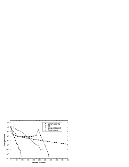
Figure 1: Convergence rate of the modified conjugated gradient method in comparing with other algorithms.

In the above calculations, we use a 3-dimensional iteration subspace for the modified CG algorithm, i.e., the subspace is constitute of the current trial vector, its corresponding gradient, as well as one previous trial vector. In such case, each iteration step needs to calculate one gradient, and some combinations of the three vectors, as well as solving a 3-dimensional eigenvalue problem. From the above argument, when the iteration subspace is 3-dimensional, the numeric cost of each iteration step is almost the same as that of the original CG method. For the block Lanczos algorithm, however, to ensure a reasonable convergence rate, the iteration subspace is 50 dimensional, i.e., one needs to calculate 50 gradients for each iteration step. To our experience, on step of Lanczos iteration needs longer CPU time than 50 steps of the modified CG method. Thus, one Lanczos step is counted as 50 steps in Figure 1.

In the 3-dimensional iteration subspace spanned by $\{|G_{n}\rangle$, $|\phi_{n}\rangle$, $|\phi_{n-1}\rangle\}$ the gradient vector $|G_{n}\rangle$, together with the previous trial vector $|\phi_{n-1}\rangle$, play the same role as that of the conjugate gradient in the minimization of a quadratic function. This is especially the case when the Rayleigh quotient closes to the minimum point, i.e., it is approximately a quadratic function of the iteration trial vector. In fact, without the previous trial vector $|\phi_{n-1}\rangle$, the lowest eigenvector obtained in the 2-dimensional subspace spanned by$\{|G_{n}\rangle,\ |\phi_{n}\rangle\}$ is just the result of steepest descent method. By including one previous trial vector which contains information about previous gradients, one is able to prevent reintroduction of errors to the refined trial vector in the direction of previous gradients. This is the reason we call this method as modified CG algorithm.

On the other hand, in the sense of relaxation algorithm for finding lowest eigenvector 4 ; 9 , the refined trial vector $|\phi_{n}\rangle$ at step $n$, is an approximation to the lowest eigenvector of the matrix in the subspace spanned by $\{|\phi_{0}\rangle,\,\,|G_{1}\rangle,\,\,|G_{2}\rangle,\,\cdots,\,\,|G_{n}\rangle\}$, which is equivalent to the subspace spanned by $\{|\phi_{0}\rangle,\,\,|\phi_{1}\rangle,\,\,|\phi_{2}\rangle,\,\,\cdots,\,|\phi_{n-1}\rangle,\,\,|\phi_{n}\rangle\}$. According to the relaxation algorithm, to find the lowest eigenvector in the subspace spanned by the above basis vectors, one starts from an initial trial vector $|\psi_{0}\rangle$, and minimizes the Rayleigh quotient iteratively. Each iterative step is to minimize the Rayleigh quotient in a two dimensional subspace spanned by the (updated) trial vector, and one basis vector. The basis vector can be chosen consecutively from the first one to the last one. After going through all basis vectors, one continues the next round of iteration by choosing the first basis vector as next basis vector. This iteration will converge after goes through all basis vectors several rounds. Note that, if one starts with the first basis vector $|\phi_{0}\rangle$ as initial trial vector, in the two dimensional subspace spanned by two consecutive basis vector $|\phi_{i}\rangle$, and $|\phi_{i+1}\rangle$, the second basis vector $|\phi_{i+1}\rangle$minimizes the Rayleigh quotient. After going through all basis vector for one round, the refined trial vector is $|\phi_{n}\rangle$, which represents an approximate lowest eigenvector in the above subspace.

The above two factors explain the rapid convergence of the modified CG algorithm. One consequence from the above arguments is that, if we increase the dimension of the iteration subspace by including more previous trial vectors, the convergence rate will not increase too much. In other words, one needs only do the modified CG algorithm in a small iteration space. To our experience, one needs at most 5-dimensional iteration subspace. In most cases, it is enough to do the iteration in the 3-dimensional iteration subspace. Figure 2 shows our numeric result to confirm this property of the modified CG algorithm. Here we do the same calculation using different iteration subspace. The filled circle connected line is the same as figure 1 with 3-dimensional iteration subspace, and the filled square and triangle are results for 6 dimensional and 12 dimensional iteration subspace respectively. There is almost no difference within 50 steps where the the convergence rate is about $10^{-8}$. One needs almost the same iteration steps to arrive the final precision. However, the 3-dimensional iteration runs faster for each iteration step since it involves less combination and production of the basis vectors that span the iteration subspace.

Figure 2: Convergence rates of the modified CG algorithm for different dimensions of the iteration subspace.

For some matrices or some properly chosen initial trial vectors, the Rayleigh quotient are approximately quadratic functions of the trial vectors. In such cases, the modified CG algorithm converges in almost the same rate as the original CG algorithm. And a trial vector $\phi_{n}$ at step $n$, is an almost exact minimum in the subspace spanned by $\{|\phi_{0}\rangle,\,|\phi_{1}\rangle,\,\cdots,\,|\phi_{n}\rangle,\,|G_{n}\rangle\}$. We have encountered such cases in our numeric tests. In fact, near a minimum, any function behaves like a quadratic function. Some matrices with special structures also make the Rayleigh quotient like a quadratic function in a quite large region of the vector space. For such matrices, the CG method is indeed a very efficient method. Of cause, in any cases the modified CG method always outperforms the original CG method.

The refined trial vector $|\phi_{n}\rangle$ becomes closer and closer to the previous step’s trial vector $|\phi_{n-1}\rangle$ when iteration closes to final solution. In higher dimensional iteration, one may encounter (numerical) degeneracy of basis vectors that span the iteration subspace. This problem is easy to solve. One simple solution is to replace this step by an steepest descent’s step. Other more sophisticated way is to choose some independent vectors from the basis vectors and do this step in a small subspace. Both methods are easy to implement. In fact, one can detect the degeneracy when solving the general form eigenvalue problem (4) which can be conveniently solved by the conventional Choleski-Householder procedure 12 . If there is a degeneracy, the Choleski decomposition of the overlap matrix $\mathcal{S}$ returns an error code. When this happens, one can simply redo this step with a steepest descent step. Alternatively, one can use a more sophisticated Choleski decomposition program that automatically chooses independent basis vector. In doing so, one must adjust the the matrix element of $\mathcal{H}$ simultaneously. This two methods need almost the same numerical cost. Of course, the first method is easy to implement. In our numerical tests, there is almost no degeneracy in the 3-dimensional iteration subspace.

It is straightforward to implement preconditioning treatment for the modified CG algorithm. Preconditioning treatment can significantly improve the convergence rate for matrices with large difference between lowest and highest eigenvalues. Due to the fact that there is no need to construct explicitly the conjugated gradient in the modified CG algorithm, it is easier to implement the preconditioning treatment by direct modifying each step’s gradient. Since preconditioning treatment depends on specific system, we don’t go into more details about such topic.

The modified CG algorithm shares a common feature with many other iterative methods of diagonalising matrices, such as Lanczos, Dividson, RMM-DIIS, and relaxation method. In all these algorithms, one refines the trial vector in iterative subspaces. What makes the modified CG algorithm different from other algorithms is that the iteration subspaces are spanned by the trial vectors of previous iteration steps, as well as the latest trial vector and its gradient. The trial vectors of previous steps are already prepared, one needs only calculating one gradient vector (and possibly does some preconditioning treatment) to construct the basis vectors of the iterative subspace. Only two basis vectors of the iterative subspace are different from previous one, it needs only update two columns of the matrix elements in the iteration subspace. By including previous trial vectors into the iterative subspace, one avoids reintroduces errors to the trial vectors in the previous directions of gradients. These properties of the iterative subspace make the modified CG algorithm numeric efficient. And the common feature of the algorithm makes it easy to implement.

It is easy to formulate block algorithm for the modified CG algorithm to find several lowest eigenvectors simultaneously. For this end, one refines several trial vectors at each iteration step. Here the iteration subspace includes all current trial vectors, their gradients, and all trial vectors of some previous steps. In this implementation, one needs to find several eigenvectors by solving the general form eigenvalue problem (4). Trial vectors obtained in this way are automatically orthogonal with each other, and one needs no additional subspace rotation.

However, one step of block algorithm usually needs more floating point operations than sequentially processing each trial vector and maintaining orthogonality between trial vectors by Schmidt orthogonalization method. This is mainly because the block algorithm needs more flops to form the matrix elements of $\mathcal{H}$ and the corresponding overlap matrix $\mathcal{S}$. If one needs $n_{0}$ lowest eigen-solutions for $N$ dimensional matrix, the block algorithm’s iterative subspace is $M=mn_{0}$ dimensional with $m=3,4,\cdots$. Each step of block algorithm needs the following floating point operations: (a) $n_{0}NL$ flops for $n_{0}$ matrix multiplying vector operations to obtain $n_{0}$ gradients, where $L\leq N$ is the band width of the matrix; (b) $2(mn_{0})^{2}N$ flops for the formation of the matrix elements of $\mathcal{H}$ in the iterative subspace and the corresponding overlap matrix $\mathcal{S}$; (c) An $O\left((mn_{0})^{3}\right)$ floating point operations for solving the general form eigen-value problem (4); (d) $2mn_{0}^{2}N$ flops for combination the $mn_{0}$ basis vectors to form $n_{0}$ refined trial vectors. Here, the flops in step (c) is negligible when $n_{0}<<N$. The total flops of one step block algorithm is $\sigma(m,n_{0},N)=n_{0}NL+2(mn_{0})^{2}N+2mn_{0}^{2}N$. If $n_{0}=1$, the above floating point operations $\sigma(m,1,N)=NL+2m^{2}N+2mN$ is the flops for processing one trial vector in sequential algorithm. One the other hand, sequentially processing each trial vector one round needs $n_{0}\sigma(m,1,N)+4n_{0}^{2}N$ flops. Here the second term is the flops to maintain the orthogonality of trial vectors, including making gradients orthogonal to previous trial vectors. Even including subspace rotation which is performed after some rounds of sequential steps, the sequential implementation needs less floating point operations than the block algorithm.

If $n_{0}$ is small, e.g., $n_{0}<10$, the difference of flops between block and sequential algorithm is small. The block algorithm may be one choice in such cases. Like the block Lanczoz 7 , and block Dividson 8 , there are some other ways to form the iterative subspace to implement the block version of modified CG algorithm. For example, the iterative subspace may contain only one gradient, plus all the current trial vectors and some previous trial vectors. The choice of iterative subspace affects the convergence properties which needs further investigations. For large $n_{0}$, e.g., $n_{0}>100$, to our experiences, block algorithm need more numeric cost and is less efficient as compared with the above sequential implementation. The dimension of the iteration subspace grows quickly with the number of needed eigenvectors, and one needs more memory to store the basis vectors and much more CPU time to solve the general from eigenvalue problem (4) which increases drastically with the dimension of the iterative subspace. Since lowest eigenvector usually converges faster that higher ones, the number of iteration steps in a block algorithm is determined by the the vector with slowest convergence rate.

IV conclusions

In summary, in the sense of conjugated gradient algorithm, we formulate an iterative method to find a set of lowest eigenvalues and eigenvectors of a matrix. This method minimizes the Rayleigh quotient of a trial vector via the gradient of the Rayleigh quotient, and at the same time, prevents reintroduce errors in the direction of previous gradients. We realize such idea by refining the trial vectors in a special kind of iteration subspaces. Each iteration subspace is spanned by the latest trial vector and the gradient of its Rayleigh quotient, as well as some trial vectors of previous steps. Each iteration step is to find lowest eigenvector in the iteration subspace. The gradient, together with the previous trial vector, play the role of the conventional conjugated gradient. In our numerical test, it is usual enough to include only one previous trial vector, i.e., one needs only refining the trail vector in a 3-dimensional subspace. As compared to the conventional conjugated gradient algorithm, which is designed to minimizes a general function, the current method exploits special properties of eigenvalue problems, and thus converges much faster in many cases. During iterations, the trial vector at the step $n$, is an approximately lowest eigenvector in the subspace spanned by the initial trial vector and $n$ subsequent gradient vectors. This is the reason of rapid convergence rate. The easy implementation of this algorithm makes it suitable for first principle calculations.

This work is supported in part by the National Natural Science Foundation, the Research Fund of the State Education Ministry of China, and the Research Fund of the Wuhan University. We thanks helpful discussions with Prof. W. Wang.

References

- (1) M. C. Payne, M. P. Teter, D. C. Allan, T. A. Arias, and J. D. Joannopoulos, Rev. Mod. Phys., 64, 1045 (1992); M. P. Teter, M. C. Patne, and D. C. Allan, Phys. Rev. B 40, 12255 (1989).
- (2) G. Kresse, and J. Furthmm̈ller, Phys. Rev. B 54, 11169 (1996).
- (3) D. M. Bylander, L. Kleinman, and S. Lee, Phys. rev. B 42, 1394 (1990).
- (4) F. Andreozzi, A. Porrino, and N. L. Iudice, J. Phys. A 35, L61, (2002).
- (5) H. Q. Lin, J. E. Gubernatis, Computers in Phys. 7, 400 (1993).
- (6) N. Wijesekera, G. Feng, T. L. Beck, arXiv:cond-mat/0304374.
- (7) J. K. Cullum, R. A. Willoughby,Lanczos Algorithms for Large Symmetric Eigenvalue Computations, (Birkhäuser Boston, Inc, 1985).
- (8) E. R. Davidson, J. Computat. Phys. 17, 87 (1975); B. Liu, in Report on the Workshop Numerical Algorithms in Chemistry: Algebraic Methods, edited by C. Moler and I. Shavitt (University of California, Berkley, 1978), p. 49.
- (9) I. Shavitt, C. F. Bender, A. Pipano, and R. P. Hosteny, J. Comput. Phys. 11, 90 (1973).
- (10) P. Pulay, Chem. Phys. Lett. 73, 393 (1980).
- (11) D. M. Wood and Z. Zunger, J. Phys. A 18, 1343 (1985).
- (12) G. H. Golub, and C. F. Van Loan, Matrix Computation, (The Johns Hopkins University Press, 1996).