Nonlinear magneto-optical rotation of frequency-modulated light resonant with a low-$J$ transition

Abstract

A low-light-power theory of nonlinear magneto-optical rotation of frequency-modulated light resonant with a $J=1\rightarrow J^{\prime}=0$ transition is presented. The theory is developed for a Doppler-free transition, and then modified to account for Doppler broadening and velocity mixing due to collisions. The results of the theory are shown to be in qualitative agreement with experimental data obtained for the rubidium $D1$ line.

I Introduction

Nonlinear magneto-optical rotation (NMOR), or light-power-dependent rotation of optical polarization due to resonant interaction with an atomic medium in the presence of a magnetic field $B$, has applications ranging from fundamental symmetry tests to magnetometry Budker et al. (2002a). With NMOR due to the evolution of ground-state atomic polarization Budker et al. (1999), optical rotation is proportional to the magnetic field for small fields, but falls off when the Larmor frequency $\Omega_{L}=g\mu_{0}B$ ($g$ is the gyromagnetic ratio, $\mu_{0}$ is the Bohr magneton, and we set $\hbar=1$ throughout) becomes larger than half of the atomic polarization relaxation rate $\gamma$ (Fig. 1).

Figure 1: Experimental (dots) and dispersive-Lorentzian least-squares fit (line) magnetic-field dependence of NMOR in a 10-cm-diameter paraffin-coated ⁸⁵Rb-vapor cell, obtained as described in Ref. Budker et al. (2000). Linearly polarized laser light is tuned to the high-frequency side of the $D2$ $F=3\rightarrow F^{\prime}$ transition, at which maximum rotation occurs. The light intensity is $\sim$50 ${\rm\mu W\,cm^{-2}}$, and the beam diameter is $\sim$2 mm. The temperature of the cell is $\sim$$19^{\circ}$C corresponding to a vapor density of $\sim$$4\times 10^{9}{\rm cm^{-3}}$.

Atomic polarization relaxation rates as low as $\gamma\simeq 2\pi\!\times 1$ Hz can be achieved for alkali atoms contained in paraffin-coated vapor cells Alexandrov et al. (1996), corresponding to magnetic field widths of approximately 1 $\mu$G Budker et al. (1998) and high magnetometric sensitivity ($\sim$3 $\rm{pG\,Hz^{-1/2}}$ Budker et al. (2000)) to small fields.

With a traditional NMOR magnetometer, the high small-field sensitivity comes at the expense of a limited dynamic range. Since many applications (such as measurement of geomagnetic fields or magnetic fields in space Ripka (2001)) require high sensitivity at magnetic fields on the order of a Gauss, a method to extend the magnetometer’s dynamic range is needed. It was recently demonstrated Budker et al. (2002b); Yashchuk et al. (2003) that when frequency-modulated light is used to induce and detect nonlinear magneto-optical rotation (FM NMOR), the narrow features in the magnetic-field dependence of optical rotation normally centered at $B=0$ can be translated to much larger magnetic fields. In this setup (Fig. 2), the light frequency is modulated at frequency $\Omega_{m}$, and the time-dependent optical rotation is measured at a harmonic of this frequency.

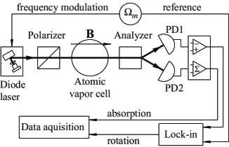
Figure 2: Simplified schematic of the apparatus used to detect FM NMOR signals. A paraffin-coated cell containing Rb vapor is placed inside a balanced polarimeter (a polarizer and an analyzer oriented at $\sim$$45^{\circ}$ with respect to each other). The frequency of the laser is modulated with an amplitude of a few dozen MHz. The lock-in amplifier is used to detect the components of optical rotation oscillating both in phase and $\pi/2$ out of phase with the frequency modulation.

Narrow features appear, centered at Larmor frequencies that are integer multiples of $\Omega_{m}$, allowing the dynamic range of the magnetometer to extend well beyond the Earth field.

Light-frequency modulation has been previously applied to measurements of linear magneto-optical rotation and parity-violating optical rotation Barkov and Zolotorev (1978); Barkov et al. (1988) in order to produce a time-dependent optical rotation signal without introducing additional optical elements (such as a Faraday modulator) between the polarizer and analyzer. Optical pumping with frequency-modulated light has been applied to magnetometry with ⁴He Cheron et al. (1995, 1996); Gilles et al. (2001) and Cs Andreeva et al. (2003); in these experiments transmission, rather than optical rotation, was monitored. In the latter work with Cs, the modulation index (the ratio of modulation depth to modulation frequency) is on the order of unity, in contrast to the much larger index in the work described here, allowing interpretation of the process in terms of the $\Lambda$- or coherent-population-trapping resonances. This regime has also been explored in Rb using modulation of the magnetic field, rather than the light field Valente et al. (2003). The closely related method of modulation of light intensity (synchronous optical pumping) predates the frequency-modulation technique Bell and Bloom (1961). Also employing light-intensity modulation is the so-called quantum beat resonance technique Aleksandrov (1963) used, for example, for measuring the Landé factors of molecular ground states (see Ref. Auzinsh and Ferber (1995) and references therein). Intensity modulation was recently used in experiments that put an upper limit on the (parity- and time-reversal-violating) electric dipole moment of ¹⁹⁹Hg (Refs. Romalis et al. (2001a, b) and references therein).

A quantitative theory of FM NMOR would be of use in the study and application of the technique. As a first step towards a complete theory, we present here a perturbative calculation for a $J=1\rightarrow J^{\prime}=0$ atomic transition that takes into account Doppler broadening and averaging due to velocity-changing collisions. We begin the discussion in Sec. II by comparing experimental FM NMOR magnetic-field-dependence data obtained with a paraffin-coated ⁸⁷Rb-vapor cell to the predictions of the calculation (described in Sec. III). We find that the simplified model still reproduces the salient features of the observed signals, indicating that the magnetic-field dependence of FM NMOR at low light power is not strongly dependent on power or angular momentum. As discussed in Sec. IV, the description of the saturation behavior and spectrum of FM NMOR in a system like Rb, on the other hand, will require a more complete theory.

II Experimental data and comparison with theory

Figures 3 and 4 show first- and second-harmonic data, respectively, obtained from an FM NMOR magnetometer with light tuned near the $D1$ line of rubidium in the manner described in Ref. Budker et al. (2002b); Yashchuk et al. (2003), along with the predicted signals for a $J=1\rightarrow J^{\prime}=0$ transition obtained from the theory described in Sec. III with parameters matching those of the experimental data.

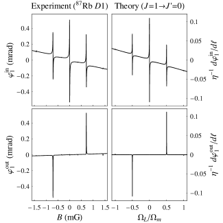
Figure 3: Measured (left column) and calculated (right column) in-phase (top row) and quadrature (bottom row) first-harmonic amplitudes of FM NMOR. The experimental signals, plotted as a function of magnetic field $B$ applied along the light propagation direction, are obtained with light tuned to the wing of the $F=2\rightarrow F^{\prime}=1$ absorption line of the ⁸⁷Rb $D1$ spectrum. The laser power is 15 $\mu$W, beam diameter is $\sim$2 mm, $\Omega_{m}=2\pi\times 1$ kHz, and modulation amplitude is $2\pi\times 220$ MHz. All resonances have widths ($\sim$1 $\mu$G) corresponding to the rate of atomic polarization relaxation in the paraffin-coated cell. The normalized calculated signals [Eq. 58], for a $J=1\rightarrow J^{\prime}=0$ transition, are plotted as a function of normalized Larmor frequency $\Omega_{L}/\Omega_{m}$. For these plots, the parameters $\Delta_{0}/\Gamma_{\!D}=0.7$, $\Omega_{m}/\gamma=500$, and $\Delta_{l}/\Delta_{0}=1$ (described in Sec. III) are chosen to match the experimental parameters given above.

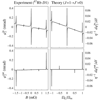
Figure 4: Measured and calculated second-harmonic amplitudes of FM NMOR. See caption to Fig. 3. For the experimental signals, light is tuned to the center of the $F=2\rightarrow F^{\prime}=1$ absorption line of the ⁸⁷Rb $D1$ spectrum, the laser power is 15 $\mu$W, beam diameter is $\sim$2.5 mm, $\Omega_{m}=2\pi\times 1$ kHz, and modulation amplitude is $2\pi\times 440$ MHz. The parameters for the theoretical signals are $\Delta_{0}/\Gamma_{\!D}=1.4$, $\Omega_{m}/\gamma=500$, and $\Delta_{l}/\Delta_{0}=0.2$.

The calculation for the simpler system reproduces many of the qualitative aspects of the experimental data for Rb. The features at the center of the in-phase plots of Figs. 3 and 4 are the zero-field resonances, analogous to the one shown in Fig. 1. (The background linear slope seen in the in-phase signals is also a zero-field resonance, due to the “transit effect” Budker et al. (2002a). It is modelled in the theory by an extra term analogous to the others with the isotropic relaxation rate $\gamma$ equal to the transit rate of atoms through the laser beam.) In addition to these features, there appear new features centered at magnetic field values at which $\left|\Omega_{L}/\Omega_{m}\right|=1/2$ and 1. For the first-harmonic signal, the former are larger, whereas for the second-harmonic, the latter are; this is primarily a result of the different light detunings used in the two measurements. For these new resonances, there are both dispersively shaped in-phase signals and $\pi/2$ out of phase (quadrature) components peaked at the centers of these resonances. The resonances occur when the optical pumping rate, which is periodic with frequency $\Omega_{m}$ due to the laser frequency modulation, is synchronized with Larmor precession, which for an aligned state has periodicity at frequency $2\Omega_{L}$ as a result of the state’s rotational symmetry. This results in the atomic medium being optically pumped into an aligned rotating state, modulating the optical properties of the medium at $2\Omega_{L}$. The aligned atoms produce maximum optical rotation when the alignment axis is at $\pi/4$ to the direction of the light polarization and no rotation when the axis is along the light polarization. Thus, on resonance, there is no in-phase signal and maximum quadrature signal. The relative sizes and signs of the features in the magnetic-field dependence, largely determined by the ratio of the modulation width $\Delta_{0}$ to the Doppler width $\Gamma_{\!D}$ (Sec. III), are well reproduced by the theory. The theory also exhibits the expected linear light-power dependence of the optical rotation amplitude as observed in experiments at low power Budker et al. (2002b); Yashchuk et al. (2003).

There are additional features, centered at $\left|\Omega_{L}/\Omega_{m}\right|=1/4$, just barely visible in the experimental plots of Figs. 3, 4. These features, which become more prominent at higher light power Yashchuk et al. (2003), are due to the optical pumping, precession, and detection of the hexadecapole moment. These resonances are not described by the current theory, because the presence of the hexadecapole moment requires ground-state angular momentum $J\geq 2$ and second-order light interactions. A quantitative description of these resonances is among the goals for an expanded theory.

III Theory

III.1 Introduction

The goals for a complete theory of FM NMOR are outlined in Sec. IV. As a first step towards such a theory, we calculate here the optical rotation due to interaction of frequency-modulated light with a $J_{g}=1\rightarrow J_{e}=0$ atomic transition (Fig. 5), where the subscripts $g$ and $e$ indicate the ground and excited states, respectively.

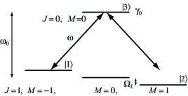
Figure 5: A $J_{g}=1\rightarrow J_{e}=0$ atomic transition of frequency $\omega_{0}$. The lower sublevels are split by the Larmor frequency $\Omega_{L}$. The arrows indicate the interaction with light of frequency $\omega$ polarized perpendicular to the quantization axis. The upper state spontaneously decays a rate $\gamma_{0}$.

We will assume that the light power is low enough that no optical pumping saturation occurs.

We begin by calculating the time-dependent atomic ground-state coherence of a Doppler-free system. Using the magnetic-field–atom and light–atom interaction Hamiltonians (under the rotating wave approximation) we write the density-matrix evolution equations. Under the low-light-power approximation, an expression for the ground-state atomic coherence can be written as a time integral. We convert the integral to a sum over harmonics of the modulation frequency by expanding the integrand as a series. This form is convenient for this calculation because the optical rotation signal is measured by lock-in detection. The expression for the Doppler-free case is then modified to take into account Doppler broadening and velocity averaging due to collisions. Atoms in an antirelaxation-coated vapor cell collide with the cell walls in between interactions with the light beam, preserving their polarization but randomizing their velocities. In the low-light-power case, we can account for this by first calculating the effect of optical pumping assuming no collisions, and then averaging the density matrix over atomic velocity. Note that in this case we assume that optical pumping is unsaturated not only for the resonant velocity group, but also when atomic polarization is averaged over the velocity distribution and cell volume.

Using the wave equation, we find an expression for the time-dependent optical rotation in terms of the atomic ground-state coherence of a given atomic velocity group. This rotation is then integrated over time and atomic velocity to obtain an expression for the signal at a given harmonic measured by the lock-in detector.

III.2 The Hamiltonian

The total Hamiltonian $H$ is the sum of the unperturbed Hamiltonian $H_{0}$, the light–atom-interaction Hamiltonian $H_{l}$, and the magnetic-field–atom-interaction Hamiltonian $H_{B}$. Using the basis states ${\left|\xi JM\right\rangle}$, where $\xi$ represents additional quantum numbers, denoted by

$${\left|\xi_{g}J_{g},-1\right\rangle} =\begin{pmatrix}1\\ 0\\ 0\\ 0\end{pmatrix}, \quad{\left|\xi_{g}J_{g},0\right\rangle} =\begin{pmatrix}0\\ 1\\ 0\\ 0\end{pmatrix},$$ (1)

$${\left|\xi_{g}J_{g},1\right\rangle} =\begin{pmatrix}0\\ 0\\ 1\\ 0\end{pmatrix}, \quad{\left|\xi_{e}J_{e},0\right\rangle} =\begin{pmatrix}0\\ 0\\ 0\\ 1\end{pmatrix},$$

the unperturbed Hamiltonian $H_{0}$ is given by

$$H_{0}=\begin{pmatrix}0&0&0&0\\ 0&0&0&0\\ 0&0&0&0\\ 0&0&0&\omega_{0}\end{pmatrix},$$ (2)

where $\omega_{0}$ is the transition frequency (again, we set $\hbar=1$ throughout).

An $x$-polarized optical electric field $\mathbf{E}$ is written as

$$\mathbf{E}=E_{0}\cos\left(\omega t\right)\hat{\mathbf{e}}_{x}.$$ (3)

where $E_{0}$ is the electric field amplitude and $\omega$ is the frequency (modulated as $\omega=\omega_{l}-\Delta_{0}\cos\Omega_{m}t$, where $\omega_{l}$ is the laser carrier frequency and $\Delta_{0}$ is the modulation amplitude). We assume that the atomic medium is optically thin, so that we can neglect the change in light polarization and intensity inside the medium when calculating the state of the medium. The light-atom interaction Hamiltonian is given by

$$\begin{split}H_{l}&{}=-\mathbf{E}\cdot\mathbf{d}\\ &{}=-E_{0}\cos\left(\omega t\right)d_{x}\\ &{}=-\frac{1}{\sqrt{2}}E_{0}\cos\left(\omega t\right)\left(d_{-1}-d_{+1}\right),\end{split}$$ (4)

where $\mathbf{d}$ is the dipole operator. According to the Wigner-Eckart theorem, components of a tensor operator $T_{\kappa q}$ are related to the reduced matrix element $\left(\xi J\|T_{\kappa}\|\xi J^{\prime}\right)$ by Sobelman (1992)

$${\left\langle\xi\!JM\right|}T_{\kappa q}{\left|\xi^{\prime}\mspace{-4.0mu}J^{\prime}\!M^{\prime}\right\rangle}=(-1)^{J-M}\!\left(\xi\!J\|T_{\kappa}\|\xi^{\prime}\mspace{-4.0mu}J^{\prime}\right)\!\begin{pmatrix}J&\kappa&J^{\prime}\\ -M&q&M^{\prime}\end{pmatrix}\mspace{-5.0mu}.$$ (5)

Thus the matrix elements of $d_{+1}$ and $d_{-1}$ for this transition can be written

$$\begin{split}&{\left\langle\xi\!JM\right|}d_{\pm 1}{\left|\xi^{\prime}\mspace{-4.0mu}J^{\prime}\!M^{\prime}\right\rangle}=(-1)^{J-M}\!\left(\xi\!J\|d\|\xi^{\prime}\mspace{-4.0mu}J^{\prime}\right)\!\begin{pmatrix}J&1&J^{\prime}\\ -M&\pm 1&M^{\prime}\end{pmatrix}\\ &=\frac{1}{\sqrt{3}}\times\begin{cases}\left(\xi_{e}J_{e}\|d\|\xi_{g}J_{g}\right)&\text{for $\xi=\xi_{e},J=J_{e},M=0$}\\ &\text{and $\xi^{\prime}=\xi_{g},J^{\prime}=J_{g},M^{\prime}=\mp 1$,}\\ \left(\xi_{g}J_{g}\|d\|\xi_{e}J_{e}\right)&\text{for $\xi=\xi_{g},J=J_{g},M=\pm 1$}\\ &\text{and $\xi^{\prime}=\xi_{e},J^{\prime}=J_{e},M^{\prime}=0$,}\\ 0&\text{in all other cases.}\end{cases}\end{split}$$ (6)

Reduced matrix elements with different ordering of states are related by Sobelman (1992)

$$\left(\xi\!J\|T_{\kappa}\|\xi^{\prime}\mspace{-4.0mu}J^{\prime}\right)=(-1)^{J-J^{\prime}}\left(\xi^{\prime}\mspace{-4.0mu}J^{\prime}\|T_{\kappa}\|\xi\!J\right)^{*},$$ (7)

and since the reduced dipole matrix element is real,

$$\left(\xi_{g}J_{g}\|d\|\xi_{e}J_{e}\right)=-\left(\xi_{e}J_{e}\|d\|\xi_{g}J_{g}\right).$$ (8)

Thus $H_{l}$ is given in matrix form by

$$H_{l}=2\Omega\cos\omega t\begin{pmatrix}0&0&0&-1\\ 0&0&0&0\\ 0&0&0&1\\ -1&0&1&0\end{pmatrix},$$ (9)

where $\Omega=\left(\xi_{g}J_{g}\|d\|\xi_{e}J_{e}\right)E_{0}/\!\left(2\sqrt{6}\,\right)$ is (apart from a numerical factor of order unity) the optical Rabi frequency.

The magnetic field interaction Hamiltonian $H_{B}$ for a $\hat{\mathbf{z}}$-directed magnetic field $\mathbf{B}$ is given by

$$\begin{split}H_{B}&{}=-\boldsymbol{\mu}\cdot\mathbf{B}\\ &{}=g\mu_{0}\,\mathbf{J}\cdot\mathbf{B}\\ &{}=g\mu_{0}J_{z}B\\ &{}=\Omega_{L}\begin{pmatrix}-1&0&0&0\\ 0&0&0&0\\ 0&0&1&0\\ 0&0&0&0\end{pmatrix},\end{split}$$ (10)

where $\Omega_{L}$ is the Larmor frequency as defined in Sec. I. Thus, the total Hamiltonian is given by

$$\begin{split}H&{}=H_{0}+H_{l}+H_{B}\\ &{}=\begin{pmatrix}-\Omega_{L}&0&0&-2\Omega\cos\omega t\\ 0&0&0&0\\ 0&0&\Omega_{L}&2\Omega\cos\omega t\\ -2\Omega\cos\omega t&0&2\Omega\cos\omega t&\omega_{0}\end{pmatrix}.\end{split}$$ (11)

III.3 Rotating-wave approximation

We now use the rotating-wave approximation in order to remove the optical-frequency time dependence from the Hamiltonian. We first transform into the frame rotating at the optical frequency by means of the unitary transformation operator $U(t)=\exp\left(-iH^{\prime}t\right)$, where

$$H^{\prime}=\begin{pmatrix}0&0&0&0\\ 0&0&0&0\\ 0&0&0&0\\ 0&0&0&\omega\end{pmatrix}$$ (12)

is the unperturbed Hamiltonian $H_{0}$ with $\omega_{0}$ replaced by $\omega$. It is straightforward to show that under this transformation the Hamiltonian in the rotating frame is given by

$$\begin{split}\tilde{H}&{}=U^{-1}(t)\,H(t)\,U(t)-i\,U^{-1}(t)\,\frac{d}{dt}\,U(t)\\ &{}=\begin{pmatrix}-\Omega_{L}&0&0&-\Omega\left(1+e^{-2i\omega t}\right)\\ 0&0&0&0\\ 0&0&\Omega_{L}&\Omega\left(1+e^{-2i\omega t}\right)\\ -\Omega\left(1+e^{2i\omega t}\right)&0&\Omega\left(1+e^{2i\omega{}t}\right)&\omega_{0}-\omega\end{pmatrix},\end{split}$$ (13)

where we have used $\cos\omega t=\left(e^{-i\omega t}+e^{i\omega t}\right)\!/\,2$. Averaging over an optical cycle to remove far-off-resonant terms (the rotating wave approximation), we have

$$\tilde{H}\simeq\begin{pmatrix}-\Omega_{L}&0&0&-\Omega\\ 0&0&0&0\\ 0&0&\Omega_{L}&\Omega\\ -\Omega&0&\Omega&-\Delta\end{pmatrix}.$$ (14)

where $\Delta=\omega-\omega_{0}$ is the (time-dependent) optical detuning.

III.4 Relaxation and repopulation

We assume that the upper state spontaneously decays with a rate $\gamma_{0}$, and that the ground state relaxes with a rate $\gamma$, due to the exit of atoms from the light beam, in the case of the “transit” effect, or collisions with other atoms or the cell wall in the case of the “wall-induced Ramsey effect” Budker et al. (2002a). (Additional upper-state relaxation processes can be neglected in comparison with the spontaneous decay rate.) This relaxation is described by the matrix $\Gamma$, given by

$$\Gamma=\begin{pmatrix}\gamma&0&0&0\\ 0&\gamma&0&0\\ 0&0&\gamma&0\\ 0&0&0&\gamma_{0}\end{pmatrix}.$$ (15)

The simplest model of ground state relaxation is used. The effects of collisional dephasing could be included by adding off-diagonal terms if a more realistic model is desired. In order to conserve the number of atoms, the ground state must be replenished at the same rate at which it relaxes. This is described by the repopulation matrix $\Lambda$:

$$\Lambda=\frac{N}{3}\begin{pmatrix}\gamma&0&0&0\\ 0&\gamma&0&0\\ 0&0&\gamma&0\\ 0&0&0&0\end{pmatrix},$$ (16)

where $N$ is the atomic density. We ignore repopulation due to spontaneous decay since the calculation is performed in the low-light-power limit ($\Omega^{2}\ll\gamma_{0}\gamma$).

III.5 Density-matrix evolution equations

The evolution of the density matrix $\rho$ (defined so that $\operatorname{Tr}\rho=N$) is given by the Liouville equation Scully and Zubairy (1997)

$$\dot{\rho}=-i\left[\tilde{H},\rho\right]-\frac{1}{2}\left\{\Gamma,\rho\right\}+\Lambda,$$ (17)

where the square brackets denote the commutator and the curly brackets the anticommutator. The $M=0$ ground-state sublevel does not couple to the light, and can be ignored. Using ${\left|1\right\rangle}$ and ${\left|2\right\rangle}$ to denote the ground-state $M=-1$ and $+1$ sublevels, respectively, and ${\left|3\right\rangle}$ to denote the upper state, and assuming that $\gamma\ll\gamma_{0}$, the evolution equations for the atomic coherences obtained from Eq. (17) are

$$\dot{\rho}_{31}=-\left[\gamma_{0}/2+i\left(\Omega_{L}-\Delta\right)\right]\rho_{31}+i\Omega\left(\rho_{11}-\rho_{33}-\rho_{21}\right),$$ (18a)

$$\dot{\rho}_{23}=-\left[\gamma_{0}/2+i\left(\Omega_{L}+\Delta\right)\right]\rho_{23}+i\Omega\left(\rho_{22}-\rho_{33}-\rho_{21}\right),$$ (18b)

$$\dot{\rho}_{21}=-\left(\gamma+2i\Omega_{L}\right)\rho_{21}-i\Omega\left(\rho_{31}+\rho_{23}\right).$$ (18c)

We can assume that in the low-light-power limit the populations $\rho_{11,22,33}$ are essentially unperturbed by the light ($\rho_{11,22}\simeq N/3$, $\rho_{33}\ll N$). We can also assume that, neglecting transient terms, the optical coherences $\rho_{31,23}$ are slowly varying (any time dependence would be due to modulation of the light frequency, which will always be done at a rate much less than $\gamma_{0}$; thus $\dot{\rho}_{31,23}\ll\gamma_{0}\rho_{31,23}$). Using these assumptions, the evolution equations for the atomic coherences [Eqs. (18a–18c)] become

$$0\simeq-\left[\gamma_{0}/2+i\left(\Omega_{L}-\Delta\right)\right]\rho_{31}+i\Omega\left(N/3-\rho_{21}\right),$$ (19a)

$$0\simeq-\left[\gamma_{0}/2+i\left(\Omega_{L}+\Delta\right)\right]\rho_{23}+i\Omega\left(N/3-\rho_{21}\right),$$ (19b)

$$\dot{\rho}_{21}{}\simeq-\left(\gamma+2i\Omega_{L}\right)\rho_{21}-i\Omega\left(\rho_{31}+\rho_{23}\right).$$ (19c)

These equations can be used to solve for the optical and ground-state coherences.

III.6 Calculation of the optical and ground-state coherences

The expression for optical rotation (Sec. III.8) is written in terms of the optical coherences $\rho_{31,23}$. We will now relate the optical coherences to the ground-state coherence $\rho_{21}$ and find an expression for $\rho_{21}$ as a sum over harmonics of the light detuning modulation frequency $\Omega_{m}$. This form is convenient because the signal is measured at harmonics of this frequency.

Solving Eqs. (19a) and (19b) for $\rho_{31}$ and $\rho_{23}$ in terms of $\rho_{21}$, we obtain

$$\begin{split}\rho_{31}&{}\simeq\frac{\Omega\left(N/3-\rho_{21}\right)}{\Omega_{L}-\Delta-i\gamma_{0}/2}\,,\\ \rho_{23}&{}\simeq\frac{\Omega\left(N/3-\rho_{21}\right)}{\Omega_{L}+\Delta-i\gamma_{0}/2}\,.\end{split}$$ (20)

In order to solve for $\rho_{21}$, we make the substitution $\rho_{21}\rightarrow r_{21}e^{-\left(2i\Omega_{L}+\gamma\right)t}$ in Eq. (19c):

$$\dot{r}_{21}\simeq-i\Omega\left(\rho_{31}+\rho_{23}\right)e^{\left(2i\Omega_{L}+\gamma\right)t},$$ (21)

or, integrating (assuming that $r_{21}=\rho_{21}=0$ at $t=0$),

$$r_{21}\simeq-i\Omega\int_{0}^{t}\left(\rho_{31}+\rho_{23}\right)e^{\left(2i\Omega_{L}+\gamma\right)\tau}d\tau,$$ (22)

so, substituting back,

$$\rho_{21}\simeq-i\Omega\int_{0}^{t}\left(\rho_{31}+\rho_{23}\right)e^{-\left(2i\Omega_{L}+\gamma\right)\left(t-\tau\right)}d\tau.$$ (23)

The expressions for the optical coherences [Eqs. (20)] are then substituted into the expression for the ground-state coherence [Eq. (23)]. Assuming that the light power is low ($\Omega\ll\gamma_{0}$) allows us to neglect second-order terms. We also assume that the level shift induced by the magnetic field is smaller than the natural line width, i.e. $\Omega_{L}\ll\gamma_{0}$. (For the $D$-lines of rubidium used in the experiment, this assumption holds for magnetic fields up to the earth-field range.) The ground-state coherence is then given by

$$\begin{split}\rho_{21}&{}\simeq-\frac{i}{3}\,\Omega^{2}N\!\int_{0}^{t}\left(\frac{1}{\Omega_{L}-\Delta-i\gamma_{0}/2}+\frac{1}{\Omega_{L}+\Delta-i\gamma_{0}/2}\right)\\ &\mspace{250.0mu}\times e^{-\left(2i\Omega_{L}+\gamma\right)\left(t-\tau\right)}d\tau\\ &{}\simeq\frac{2}{3}\,\Omega^{2}N\!\int_{0}^{t}\left(\frac{\gamma_{0}/2-i\Omega_{L}}{\Delta\mspace{-1.0mu}^{2}+\gamma_{0}^{2}/4}+\frac{2i\Omega_{L}\Delta\mspace{-1.0mu}^{2}}{\left(\Delta\mspace{-1.0mu}^{2}+\gamma_{0}^{2}/4\right)^{2}}\right)\\ &\mspace{250.0mu}\times e^{-\left(2i\Omega_{L}+\gamma\right)\left(t-\tau\right)}d\tau\\ &=\frac{2}{3}\,\Omega^{2}N\left[\left(\gamma_{0}/2-i\Omega_{L}\right)I_{1}(t)+2i\Omega_{L}I_{2}(t)\right],\end{split}$$ (24)

where the integral $I_{1}$ has been defined by

$$\begin{split}I_{1}(t)&=\int_{0}^{t}\frac{e^{-\left(2i\Omega_{L}+\gamma\right)\left(t-\tau\right)}\,d\tau}{\Delta_{0}^{2}\left(D_{0}-\cos\Omega_{m}\tau\right)^{2}+\gamma_{0}^{2}/4}\,\\ &=\left(\gamma_{0}^{2}/4\right)^{-1}\int_{0}^{t}f\!\left(\Omega_{m}\tau\right)\,e^{-\left(2i\Omega_{L}+\gamma\right)\left(t-\tau\right)}\,d\tau,\end{split}$$ (25)

and $I_{2}$ has been defined by

$$\begin{split}I_{2}(t)&=\mspace{-5.0mu}\int_{0}^{t}\mspace{-7.0mu}\frac{\Delta_{0}^{2}\left(D_{0}-\cos\Omega_{m}\tau\right)^{2}d\tau}{\left[\Delta_{0}^{2}\left(D_{0}-\cos\Omega_{m}\tau\right)^{2}+\gamma_{0}^{2}/4\right]^{2}}\,e^{-\left(2i\Omega_{L}+\gamma\right)\left(t-\tau\right)}\\ &=-\Delta_{0}^{2}\frac{\partial I_{1}(t)}{\partial\Delta_{0}^{2}}.\end{split}$$ (26)

Here we have substituted for $\Delta$ the expression for the light-frequency modulation $\Delta=\Delta_{0}\left(D_{0}-\cos\Omega_{m}\tau\right)$, where the dimensionless average detuning parameter $D_{0}$ is defined by $D_{0}=\Delta_{l}/\Delta_{0}$, where $\Delta_{l}=\omega_{l}-\omega_{0}$. The lineshape factor $f(x)$ is defined by

$$f(x)=\frac{\gamma_{0}^{2}/4}{\Delta_{0}^{2}\left(D_{0}-\cos x\right)^{2}+\gamma_{0}^{2}/4}.$$ (27)

Expanding this function as a series of harmonics,

$$f(x)=\sum_{n=-\infty}^{\infty}a_{n}e^{inx},$$ (28)

the coefficients $a_{n}$ are given by

$$a_{n}=\frac{1}{2\pi}\int_{-\pi}^{\pi}f(x)\,\cos nx\,dx.$$ (29)

Substituting the series expansion for $f(x)$ into $I_{1}$, we have

$$\begin{split}I_{1}(t)&{}\simeq\int_{0}^{t}\left[\left(\gamma_{0}^{2}/4\right)^{-1}\mspace{-8.0mu}\sum_{n=-\infty}^{\infty}a_{n}e^{in\Omega_{m}\tau}\right]e^{-\left(2i\Omega_{L}+\gamma\right)\left(t-\tau\right)}d\tau\\ &=\left(\gamma_{0}^{2}/4\right)^{-1}\mspace{-8.0mu}\sum_{n=-\infty}^{\infty}\frac{e^{in\Omega_{m}t}-e^{-\left(\gamma+2i\Omega_{L}\right)t}}{\gamma+i\left(2\Omega_{L}+n\Omega_{m}\right)}\,a_{n}\\ &{}\simeq\left(\gamma_{0}^{2}/4\right)^{-1}\mspace{-8.0mu}\sum_{n=-\infty}^{\infty}\frac{a_{n}e^{in\Omega_{m}t}}{\gamma+i\left(2\Omega_{L}+n\Omega_{m}\right)}\,,\end{split}$$ (30)

where we have discarded the transient term $e^{-\left(\gamma+2i\Omega_{L}\right)t}$. The expression for $I_{2}$ [Eq. (26)] can be found from that for $I_{1}$:

$$\begin{split}I_{2}(t)&=-\Delta_{0}^{2}\frac{\partial I_{1}(t)}{\partial\Delta_{0}^{2}}\\ &{}\simeq\left(\gamma_{0}^{2}/4\right)^{-1}\mspace{-8.0mu}\sum_{n=-\infty}^{\infty}\frac{b_{n}e^{in\Omega_{m}t}}{\gamma+i\left(2\Omega_{L}+n\Omega_{m}\right)}\,,\end{split}$$ (31)

where the coefficient $b_{n}$ is defined by

$$b_{n}=-\Delta_{0}^{2}\frac{\partial a_{n}}{\partial\Delta_{0}^{2}}$$ (32)

In order to find the relative values of $a_{n}$ and $b_{n}$, it is useful to have an approximate expression for them. Assuming that $\gamma_{0}\ll\Delta_{0}$, we can replace $f(x)$ with a delta function normalized to the same area:

$$f(x)\simeq\frac{\pi\gamma_{0}}{2\Delta_{0}\sqrt{1-D_{0}^{2}}}\,\delta\!\left(D_{0}-\cos x\right).$$ (33)

Substituting this expression into Eq. (29), we obtain

$$a_{n}\simeq\frac{\gamma_{0}}{2\Delta_{0}}\frac{\cos\left(n\arccos{D_{0}}\right)}{\sqrt{1-D_{0}^{2}}}.$$ (34)

This approximation breaks down for $\left|D_{0}\right|$ within $\sim$$\gamma_{0}/\Delta_{0}$ of unity. However, as we see below, we are interested in integrals of $a_{n}$ over effective detuning, which can be well approximated using the expression (34). We are also limited by this approximation to harmonics $n\ll\Delta_{0}/\gamma_{0}$, since the factor $\cos nx$ is assumed to not vary rapidly over the optical resonance. Thus, from Eq. (32), $b_{n}$ can be approximated by

$$\begin{split}b_{n}&{}\simeq\frac{\gamma_{0}}{4\Delta_{0}}\frac{\cos\left(n\arccos{D_{0}}\right)}{\sqrt{1-D_{0}^{2}}}\\ &{}\simeq\frac{1}{2}\,a_{n}.\end{split}$$ (35)

Thus we see that $I_{2}\simeq I_{1}/2$ and the terms of Eq. (24) proportional to $\Omega_{L}$ cancel. Substituting Eq. (30) into Eq. (24), we obtain

$$\rho_{21}\simeq\frac{4\Omega^{2}N}{3\gamma_{0}}\!\sum_{n=-\infty}^{\infty}\frac{a_{n}\,e^{in\Omega_{m}t}}{\gamma+i\left(2\Omega_{L}+n\Omega_{m}\right)}\,.$$ (36)

The result (36) applies to atoms that are at rest. We now modify this result to describe an atomic ensemble with a Maxwellian velocity distribution leading to a Doppler width $\Gamma_{\!D}$ of the transition. For an atomic velocity group with component of velocity $v$ along the light propagation direction, the light frequency is shifted according to $\omega(v)=\omega\left(1-v/c\right)=\omega-kv$ where $k$ is the light-field wave number. Writing the dimensionless Doppler-shift parameter $D_{v}=-kv/\Delta_{0}$, the atomic density $N$ for this velocity group becomes

$$dN(v)=\frac{\Delta_{0}}{\Gamma_{\!D}\sqrt{\pi}}\,N_{0}\,e^{-\left(D_{v}\Delta_{0}/\Gamma_{\!D}\right)^{2}}\,dD_{v},$$ (37)

where $N_{0}$ is the total atomic density, and the average detuning parameter $D_{0}$ becomes $D_{0}(v)=D_{0}+D_{v}$. Defining the velocity-dependent coefficient $a_{n}\mspace{-1.0mu}(v)$ by

$$\begin{split}a_{n}\mspace{-1.0mu}(v)\,dD_{v}&=\frac{\Gamma_{\!D}}{\gamma_{0}}\frac{dN(v)}{N_{0}}\,a_{n}\\ &{}\simeq\frac{\cos\left[n\arccos\left(D_{0}+D_{v}\right)\right]}{2\sqrt{\pi}\sqrt{1-\left(D_{0}+D_{v}\right)^{2}}}\,e^{-\left(D_{v}\Delta_{0}/\Gamma_{\!D}\right)^{2}}dD_{v},\end{split}$$ (38)

the velocity-dependent ground-state coherence $\rho_{21}\mspace{-1.0mu}(v)$ is given by

$$\begin{split}\rho_{21}\mspace{-1.0mu}(v)\,dD_{v}&{}\simeq\frac{4\Omega^{2}\,d\mspace{-1.0mu}N\mspace{-1.0mu}(v)}{3\gamma_{0}}\!\sum_{n=-\infty}^{\infty}\frac{a_{n}\,e^{in\Omega_{m}t}}{\gamma+i\left(2\Omega_{L}+n\Omega_{m}\right)}\\ &{}\simeq\frac{4\Omega^{2}N_{0}}{3\Gamma_{\!D}}\!\sum_{n=-\infty}^{\infty}\frac{a_{n}\mspace{-1.0mu}(v)\,e^{in\Omega_{m}t}}{\gamma+i\left(2\Omega_{L}+n\Omega_{m}\right)}\,dD_{v}.\end{split}$$ (39)

In a situation in which atomic collisions are important, such as in a vapor cell with a buffer gas or an antirelaxation coating, this result must be further modified to take into account collisionally induced velocity mixing. For atoms contained in an antirelaxation-coated vapor cell, we assume that each velocity group interacts separately with the excitation light, but after pumping all groups are completely mixed. This model applies when light power is low enough so that optical pumping averaged over the atomic velocity distribution and the cell volume is unsaturated. The ground-state coherence of each velocity group becomes the velocity-averaged quantity $\bar{\rho}_{21}\mspace{-1.0mu}(v)$, given by the normalized velocity average of Eq. (39):

$$\begin{split}\bar{\rho}_{21}\mspace{-1.0mu}(v)\,dD_{v}&{}\simeq\frac{dN(v)}{N_{0}}\int_{-\infty}^{\infty}\rho_{21}\mspace{-1.0mu}(v)\,dD_{v}\\ &{}=\frac{4\Omega^{2}\,d\mspace{-1.0mu}N\mspace{-1.0mu}(v)}{3\Gamma_{\!D}}\sum_{n=-\infty}^{\infty}\frac{\bar{a}_{n}\,e^{in\Omega_{m}t}}{\gamma+i\left(2\Omega_{L}+n\Omega_{m}\right)}\,,\end{split}$$ (40)

where the averaged coefficient $\bar{a}_{n}$ is given by

$$\begin{split}\bar{a}_{n}&=\int_{-\infty}^{\infty}a_{n}\mspace{-1.0mu}(v)\,dD_{v}\\ &{}\simeq\int_{-\infty}^{\infty}\frac{\cos\left[n\arccos\left(D_{0}+D_{v}\right)\right]}{2\sqrt{\pi}\sqrt{1-\left(D_{0}+D_{v}\right)^{2}}}\,e^{-\left(D_{v}\Delta_{0}/\Gamma_{\!D}\right)^{2}}\,dD_{v}.\end{split}$$ (41)

Below, we will need the real and imaginary parts of $\bar{\rho}_{21}$, given by

$$\begin{split}\operatorname{Re}{}&\bar{\rho}_{21}\mspace{-1.0mu}(v)\,dD_{v}\simeq\frac{4\Omega^{2}\,d\mspace{-1.0mu}N\mspace{-1.0mu}(v)}{3\Gamma_{\!D}}\\ &{}\times\sum_{n=-\infty}^{\infty}\frac{\bar{a}_{n}\left[\gamma\cos n\Omega_{m}t+\left(2\Omega_{L}+n\Omega_{m}\right)\sin n\Omega_{m}t\right]}{\gamma^{2}+\left(2\Omega_{L}+n\Omega_{m}\right)^{2}}\,,\\ \operatorname{Im}{}&\bar{\rho}_{21}\mspace{-1.0mu}(v)\,dD_{v}\simeq\frac{4\Omega^{2}\,d\mspace{-1.0mu}N\mspace{-1.0mu}(v)}{3\Gamma_{\!D}}\\ &{}\times\sum_{n=-\infty}^{\infty}\frac{\bar{a}_{n}\left[\gamma\sin n\Omega_{m}t-\left(2\Omega_{L}+n\Omega_{m}\right)\cos n\Omega_{m}t\right]}{\gamma^{2}+\left(2\Omega_{L}+n\Omega_{m}\right)^{2}}\,.\end{split}$$ (42)

III.7 Optical properties of the medium

We now derive the formula for the optical rotation in terms of the polarization of the medium $\mathbf{P}=\operatorname{Tr}\rho\mathbf{d}$. The electric field of coherent light of arbitrary polarization can be described by Huard (1997)

$$\begin{split}\mathbf{E}&{}=\frac{1}{2}\left[E_{0}e^{i\phi}\left(\cos\varphi\cos\epsilon-i\sin\varphi\sin\epsilon\right)e^{i\left(\omega t-kz\right)}+c.c.\right]\hat{\mathbf{e}}_{x}\\ &{}+\frac{1}{2}\left[E_{0}e^{i\phi}\left(\sin\varphi\cos\epsilon+i\cos\varphi\sin\epsilon\right)e^{i\left(\omega t-kz\right)}+c.c.\right]\hat{\mathbf{e}}_{y},\end{split}$$ (43)

where $k=\omega/c$ is the vacuum wave number, $\phi$ is the overall phase, $\varphi$ is the polarization angle, and $\epsilon$ is the ellipticity.

Substituting Eq. (43) into the wave equation

$$\left(\frac{d^{2}}{dz^{2}}-\frac{d^{2}}{c^{2}dt^{2}}\right)\mathbf{E}=-\frac{4\pi}{c^{2}}\frac{d^{2}}{dt^{2}}\mathbf{P},$$ (44)

and neglecting terms involving second-order derivatives and products of first-order derivatives (thus assuming that changes in $\varphi$, $\epsilon$, and $\phi$ and fractional changes in $E_{0}$ are small), gives the rotation, phase shift, absorption, and change of ellipticity per unit distance:

$$\begin{split}\frac{d\varphi}{dz}=&-\frac{2\pi\omega}{E_{0}c}\sec 2\epsilon\left[\cos\varphi\left(P_{1}\sin\epsilon+P_{4}\cos\epsilon\right)\right.\\ &\mspace{150.0mu}\left.{}-\sin\varphi\left(P_{2}\cos\epsilon-P_{3}\sin\epsilon\right)\right],\\ \frac{d\phi}{dz}=&-\frac{2\pi\omega}{E_{0}c}\sec 2\epsilon\left[\cos\varphi\left(P_{1}\cos\epsilon+P_{4}\sin\epsilon\right)\right.\\ &\mspace{150.0mu}\left.{}-\sin\varphi\left(P_{2}\sin\epsilon-P_{3}\cos\epsilon\right)\right],\\ \frac{dE_{0}}{dz}=&\frac{2\pi\omega}{c}\left[\sin\varphi\left(P_{1}\sin\epsilon-P_{4}\cos\epsilon\right)\right.\\ &\mspace{150.0mu}\left.{}-\cos\varphi\left(P_{2}\cos\epsilon+P_{3}\sin\epsilon\right)\right],\\ \frac{d\epsilon}{dz}=&\frac{2\pi\omega}{E_{0}c}\left[\sin\varphi\left(P_{1}\cos\epsilon+P_{4}\sin\epsilon\right)\right.\\ &\mspace{150.0mu}\left.{}+\cos\varphi\left(P_{2}\sin\epsilon-P_{3}\cos\epsilon\right)\right],\end{split}$$ (45)

where the components $P_{1,2,3,4}$ of the polarization are defined by

$$\begin{split}\mathbf{P}&{}=\frac{1}{2}\left[\left(P_{1}-iP_{2}\right)e^{i\left(\omega t-kz\right)}+c.c.\right]\hat{\mathbf{e}}_{x}\\ &{}+\frac{1}{2}\left[\left(P_{3}-iP_{4}\right)e^{i\left(\omega t-kz\right)}+c.c.\right]\hat{\mathbf{e}}_{y}.\end{split}$$ (46)

For initial values of $\varphi=\epsilon=0$, the rotation per unit length is given by

$$\frac{d\varphi}{d\ell}=-\frac{2\pi\omega P_{4}}{cE_{0}}\,.$$ (47)

III.8 Calculation of the signal

We now evaluate $\mathbf{P}=\operatorname{Tr}\rho\mathbf{d}$ and substitute into Eq. (47) to find the optical rotation in terms of the ground-state atomic coherence derived above. Taking into account that in the nonrotating frame the optical atomic coherences oscillate at the light frequency $\omega$, we find for the polarization components

$$\begin{split}P_{1}&=\sqrt{\frac{2}{3}}\left(\xi_{g}J_{g}\|d\|\xi_{e}J_{e}\right)\operatorname{Re}\left(\rho_{31}-\rho_{23}\right),\\ P_{2}&=-\sqrt{\frac{2}{3}}\left(\xi_{g}J_{g}\|d\|\xi_{e}J_{e}\right)\operatorname{Im}\left(\rho_{31}+\rho_{23}\right),\\ P_{3}&=-\sqrt{\frac{2}{3}}\left(\xi_{g}J_{g}\|d\|\xi_{e}J_{e}\right)\operatorname{Im}\left(\rho_{31}-\rho_{23}\right),\\ P_{4}&=-\sqrt{\frac{2}{3}}\left(\xi_{g}J_{g}\|d\|\xi_{e}J_{e}\right)\operatorname{Re}\left(\rho_{31}+\rho_{23}\right),\end{split}$$ (48)

so the optical rotation angle per unit length is given by

$$\begin{split}\frac{d\varphi}{d\ell}&=\frac{\pi\omega\left(\xi_{g}J_{g}\|d\|\xi_{e}J_{e}\right)^{2}}{3\Omega c}\operatorname{Re}\left(\rho_{31}+\rho_{32}\right)\\ &=\frac{\gamma_{0}\lambda^{2}}{16\pi\Omega}\operatorname{Re}\left(\rho_{31}+\rho_{32}\right),\end{split}$$ (49)

where $\lambda$ is the transition wavelength. Here we have used the fact that for a closed $J\rightarrow J^{\prime}$ transition Sobelman (1992),

$$\gamma_{0}=\frac{4\mspace{1.0mu}\omega_{0}^{3}}{3\mspace{1.0mu}c^{3}}\frac{1}{2J^{\prime}+1}\left(\xi\!J\|d\|\xi^{\prime}\mspace{-4.0mu}J^{\prime}\right)^{2},$$ (50)

and that $\omega\simeq\omega_{0}$.

Substituting in the expressions (20), and assuming $\rho_{11}\simeq\rho_{22}\simeq N/3$ and $\Omega_{L}\ll\gamma_{0}$, Eq. (49) can be written in terms of the ground-state coherence as

$$\frac{d\varphi}{d\ell}=\frac{\gamma_{0}\lambda^{2}}{8\pi}\left(\frac{\Omega_{L}\left(N/3-\operatorname{Re}\rho_{21}\right)+\left(\gamma_{0}/2\right)\operatorname{Im}\rho_{21}}{\gamma_{0}^{2}/4+\Delta\mspace{-1.0mu}^{2}}-\frac{2\Omega_{L}\Delta\mspace{-1.0mu}^{2}\left(N/3-\operatorname{Re}\rho_{21}\right)}{\left(\gamma_{0}^{2}/4+\Delta\mspace{-1.0mu}^{2}\right)^{2}}\right),$$ (51)

or, for the case of complete velocity mixing:

$$\frac{d\varphi(v)}{d\ell}\,dD_{v}=\frac{\gamma_{0}\lambda^{2}}{8\pi}\left(\frac{\Omega_{L}\left[dN(v)/3-\operatorname{Re}\bar{\rho}_{21}\mspace{-1.0mu}(v)\,dD_{v}\right]+\left(\gamma_{0}/2\right)\operatorname{Im}\bar{\rho}_{21}\mspace{-1.0mu}(v)\,dD_{v}}{\gamma_{0}^{2}/4+\Delta\mspace{-1.0mu}^{2}(v)}-\frac{2\Omega_{L}\Delta\mspace{-1.0mu}^{2}(v)\left[dN(v)/3-\operatorname{Re}\bar{\rho}_{21}\mspace{-1.0mu}(v)\,dD_{v}\right]}{\left[\gamma_{0}^{2}/4+\Delta\mspace{-1.0mu}^{2}(v)\right]^{2}}\right),$$ (52)

where the velocity-dependent effective detuning $\Delta(v)$ is given, as before, by

$$\Delta(v)=\Delta_{0}\left[D_{0}(v)-\cos\Omega_{m}\tau\right].$$ (53)

The in-phase and quadrature signals (see Sec. II) per unit length of the medium, measured for a time $T$ at the $j$-th harmonic of the modulation frequency, are given by the time averages

$$\begin{split}\frac{d\varphi^{\text{in}}_{\!j}(v)}{d\ell}\,dD_{v}&{}=\frac{dD_{v}}{T}\int_{0}^{T}\frac{d\varphi(v)}{d\ell}\cos\left(j\,\Omega_{m}t\right)dt,\\ \frac{d\varphi^{\text{out}}_{\!j}(v)}{d\ell}\,dD_{v}&{}=\frac{dD_{v}}{T}\int_{0}^{T}\frac{d\varphi(v)}{d\ell}\sin\left(j\,\Omega_{m}t\right)dt.\end{split}$$ (54)

We substitute the formulas for the real and imaginary parts of the ground-state coherence [Eq. (42)] into the formula for the optical rotation [Eq. (52)], and the resulting expression into Eq. (54). After evaluating the time integrals (see Appendix A), we find that the signals due to each velocity group are given by

$$\begin{split}\frac{d\varphi^{\text{in}}_{\!j}(v)}{d\ell}\,dD_{v}\simeq{}&-\frac{\lambda^{2}\Omega^{2}}{6\pi\Gamma_{\!D}}\,dN(v)\\ &{}\times\sum_{n=-\infty}^{\infty}\mspace{-6.0mu}\frac{\left(2\Omega_{L}+n\Omega_{m}\right)\bar{a}_{n}\left(a_{n+j}+a_{n-j}\right)}{\gamma^{2}+\left(2\Omega_{L}+n\Omega_{m}\right)^{2}},\\ \frac{d\varphi^{\text{out}}_{\!j}(v)}{d\ell}\,dD_{v}\simeq{}&-\frac{\lambda^{2}\Omega^{2}}{6\pi\Gamma_{\!D}}\,dN(v)\\ &{}\times\sum_{n=-\infty}^{\infty}\mspace{-6.0mu}\frac{\gamma\,\bar{a}_{n}\left(a_{n+j}-a_{n-j}\right)}{\gamma^{2}+\left(2\Omega_{L}+n\Omega_{m}\right)^{2}}\,.\end{split}$$ (55)

Using the definitions of $dN(v)$ and $a_{n}\mspace{-1.0mu}(v)$ [Eqs. (37,38)] we can rewrite Eq. (55) as

$$\begin{split}&\frac{d\varphi^{\text{in}}_{\!j}(v)}{d\ell}\,dD_{v}\\ &\mspace{10.0mu}{}\simeq\eta\!\!\sum_{n=-\infty}^{\infty}\mspace{-6.0mu}\frac{\gamma\left(2\Omega_{L}+n\Omega_{m}\right)\bar{a}_{n}\left[a_{n+j}\mspace{-1.0mu}(v)+a_{n-j}\mspace{-1.0mu}(v)\right]}{\gamma^{2}+\left(2\Omega_{L}+n\Omega_{m}\right)^{2}}\,dD_{v},\\ &\frac{d\varphi^{\text{out}}_{\!j}(v)}{d\ell}\,dD_{v}\\ &\mspace{10.0mu}{}\simeq\eta\!\!\sum_{n=-\infty}^{\infty}\mspace{-6.0mu}\frac{\gamma^{2}\,\bar{a}_{n}\left[a_{n+j}\mspace{-1.0mu}(v)-a_{n-j}\mspace{-1.0mu}(v)\right]}{\gamma^{2}+\left(2\Omega_{L}+n\Omega_{m}\right)^{2}}\,\,dD_{v},\end{split}$$ (56)

where the signal amplitude factor $\eta$ is defined by

$$\eta=-\frac{1}{6\pi}\frac{\Omega^{2}\gamma_{0}}{\Gamma_{\!D}^{2}\gamma}\,\lambda^{2}\!N_{0}.$$ (57)

The total signal, given by the integral over all velocity groups, is found by replacing $a_{n}\mspace{-1.0mu}(v)$ with $\bar{a}_{n}$:

$$\begin{split}\left.\frac{d\varphi^{\text{in}}_{\!j}}{d\ell}\right|_{\text{total}}&=\int_{-\infty}^{\infty}\frac{d\varphi_{\text{in}}(v)}{d\ell}\,dD_{v}\\ &\simeq\eta\!\!\sum_{n=-\infty}^{\infty}\mspace{-6.0mu}\frac{\gamma\left(2\Omega_{L}+n\Omega_{m}\right)\bar{a}_{n}\left(\bar{a}_{n+j}+\bar{a}_{n-j}\right)}{\gamma^{2}+\left(2\Omega_{L}+n\Omega_{m}\right)^{2}},\\ \left.\frac{d\varphi^{\text{out}}_{\!j}}{d\ell}\right|_{\text{total}}&=\int_{-\infty}^{\infty}\frac{d\varphi_{\text{out}}(v)}{d\ell}\,dD_{v}\\ &\simeq\eta\!\!\sum_{n=-\infty}^{\infty}\mspace{-6.0mu}\frac{\gamma^{2}\,\bar{a}_{n}\left(\bar{a}_{n+j}-\bar{a}_{n-j}\right)}{\gamma^{2}+\left(2\Omega_{L}+n\Omega_{m}\right)^{2}}\,.\end{split}$$ (58)

Each term of the sums corresponds to a resonance at $\Omega_{L}/\Omega_{m}=-n/2$ (Figs. 3,4). Near each resonance the in-phase signal is dispersive in shape, whereas the quadrature signal is a Lorentzian. When plotted as a function of the Larmor frequency normalized to the modulation frequency, $\Omega_{L}/\Omega_{m}$, the widths of the resonances are determined by the normalized ground-state relaxation rate $\gamma/\Omega_{m}$. The relative amplitudes of the resonances are determined by the ratio of the modulation depth to the Doppler width, $\Delta_{0}/\Gamma_{\!D}$, and the normalized average detuning $\Delta_{l}/\Delta_{0}$.

IV Conclusion

We have presented a theory of nonlinear magneto-optical rotation with low-power frequency-modulated light for a low-angular-momentum system. The magnetic-field dependence predicted by this theory is in qualitative agreement with experimental data taken on the Rb $D1$ line. Directions for future work include a more complete theory describing higher-angular-momentum systems, including systems with hyperfine structure, and higher light powers. A possible complication to the FM NMOR technique in systems with hyperfine structure is the nonlinear Zeeman effect present at higher magnetic fields, so a theoretical description of this effect would also be helpful. FM NMOR has been shown to be a useful technique for the selective study of higher-order polarization moments, which give rise to distinct resonances at different values of the magnetic field than the quadrupole resonances studied here Yashchuk et al. (2003) (see also Ref. Auzin’sh and Ferber (1984)). Higher-order moments are of interest in part because signals due to the highest-order moments possible in a given system would be free of the complications due to the nonlinear Zeeman effect. To describe these moments, a calculation along the same lines as the one presented here but carried out to higher order and involving more atomic sublevels would be necessary.

Appendix A Evaluation of the time integrals

In evaluating Eq. (54), several time integrals appear:

$$I_{3}=\frac{1}{\Omega_{m}T}\int_{0}^{\Omega_{m}T}\frac{\cos jx}{\gamma_{0}^{2}/4+\Delta_{0}^{2}\left[D_{0}(v)-\cos x\right]^{2}}\,dx,$$

$$I_{4}=\frac{1}{\Omega_{m}T}\int_{0}^{\Omega_{m}T}\frac{\sin jx}{\gamma_{0}^{2}/4+\Delta_{0}^{2}\left[D_{0}(v)-\cos x\right]^{2}}\,dx,$$

$$I_{5}=\frac{1}{\Omega_{m}T}\int_{0}^{\Omega_{m}T}\frac{\cos jx\sin nx}{\gamma_{0}^{2}/4+\Delta_{0}^{2}\left[D_{0}(v)-\cos x\right]^{2}}\,dx,$$

$$I_{6}=\frac{1}{\Omega_{m}T}\int_{0}^{\Omega_{m}T}\frac{\sin jx\sin nx}{\gamma_{0}^{2}/4+\Delta_{0}^{2}\left[D_{0}(v)-\cos x\right]^{2}}\,dx,$$

$$I_{7}=\frac{1}{\Omega_{m}T}\int_{0}^{\Omega_{m}T}\frac{\cos jx\cos nx}{\gamma_{0}^{2}/4+\Delta_{0}^{2}\left[D_{0}(v)-\cos x\right]^{2}}\,dx,$$

$$I_{8}=\frac{1}{\Omega_{m}T}\int_{0}^{\Omega_{m}T}\frac{\sin jx\cos nx}{\gamma_{0}^{2}/4+\Delta_{0}^{2}\left[D_{0}(v)-\cos x\right]^{2}}\,dx,$$

as well as the related integrals

$$\begin{split}I_{9}&=\frac{1}{\Omega_{m}T}\int_{0}^{\Omega_{m}T}\frac{\Delta_{0}^{2}\left[D_{0}(v)-\cos x\right]^{2}\cos jx}{\left\{\gamma_{0}^{2}/4+\Delta_{0}^{2}\left[D_{0}(v)-\cos x\right]^{2}\right\}^{2}}\,dx\\ &=-\Delta_{0}^{2}\frac{\partial I_{3}}{\partial\Delta_{0}^{2}},\end{split}$$

$$\begin{split}I_{10}&=\frac{1}{\Omega_{m}T}\int_{0}^{\Omega_{m}T}\frac{\Delta_{0}^{2}\left[D_{0}(v)-\cos x\right]^{2}\sin jx}{\left\{\gamma_{0}^{2}/4+\Delta_{0}^{2}\left[D_{0}(v)-\cos x\right]^{2}\right\}^{2}}\,dx\\ &=-\Delta_{0}^{2}\frac{\partial I_{4}}{\partial\Delta_{0}^{2}},\end{split}$$

$$\begin{split}I_{11}&=\frac{1}{\Omega_{m}T}\int_{0}^{\Omega_{m}T}\frac{\Delta_{0}^{2}\left[D_{0}(v)-\cos x\right]^{2}\cos jx\sin nx}{\left\{\gamma_{0}^{2}/4+\Delta_{0}^{2}\left[D_{0}(v)-\cos x\right]^{2}\right\}^{2}}\,dx\\ &=-\Delta_{0}^{2}\frac{\partial I_{5}}{\partial\Delta_{0}^{2}},\end{split}$$

$$\begin{split}I_{12}&=\frac{1}{\Omega_{m}T}\int_{0}^{\Omega_{m}T}\frac{\Delta_{0}^{2}\left[D_{0}(v)-\cos x\right]^{2}\sin jx\sin nx}{\left\{\gamma_{0}^{2}/4+\Delta_{0}^{2}\left[D_{0}(v)-\cos x\right]^{2}\right\}^{2}}\,dx\\ &=-\Delta_{0}^{2}\frac{\partial I_{6}}{\partial\Delta_{0}^{2}},\end{split}$$

$$\begin{split}I_{13}&=\frac{1}{\Omega_{m}T}\int_{0}^{\Omega_{m}T}\frac{\Delta_{0}^{2}\left[D_{0}(v)-\cos x\right]^{2}\cos jx\cos nx}{\left\{\gamma_{0}^{2}/4+\Delta_{0}^{2}\left[D_{0}(v)-\cos x\right]^{2}\right\}^{2}}\,dx\\ &=-\Delta_{0}^{2}\frac{\partial I_{7}}{\partial\Delta_{0}^{2}},\end{split}$$

$$\begin{split}I_{14}&=\frac{1}{\Omega_{m}T}\int_{0}^{\Omega_{m}T}\frac{\Delta_{0}^{2}\left[D_{0}(v)-\cos x\right]^{2}\sin jx\cos nx}{\left\{\gamma_{0}^{2}/4+\Delta_{0}^{2}\left[D_{0}(v)-\cos x\right]^{2}\right\}^{2}}\,dx\\ &=-\Delta_{0}^{2}\frac{\partial I_{8}}{\partial\Delta_{0}^{2}}.\end{split}$$

If $T$ is many modulation periods, the above integrals can be approximated by averages over one period. Thus, we can change the limits of the integrals to $\left(-\pi,\pi\right)$, and set the normalizing factor $\left(\Omega_{m}T\right)^{-1}$ to $\left(2\pi\right)^{-1}$. Using the trigonometric substitutions

$$\begin{split}\cos jx\cos nx&{}=\frac{1}{2}\left\{\cos\left[\left(n-j\right)x\right]+\cos\left[\left(n+j\right)x\right]\right\},\\ \cos jx\sin nx&{}=\frac{1}{2}\left\{\sin\left[\left(n-j\right)x\right]+\sin\left[\left(n+j\right)x\right]\right\},\\ \sin jx\sin nx&{}=\frac{1}{2}\left\{\cos\left[\left(n-j\right)x\right]-\cos\left[\left(n+j\right)x\right]\right\},\\ \sin jx\cos nx&{}=-\frac{1}{2}\left\{\sin\left[\left(n-j\right)x\right]+\sin\left[\left(n+j\right)x\right]\right\},\end{split}$$ (59)

we can rewrite the above integrals in terms of the $a_{n}$ and $b_{n}$ coefficients.

$$\begin{split}I_{3}&{}\simeq\left(\gamma_{0}^{2}/4\right)^{-1}a_{j},\\ I_{4}&{}\simeq 0,\\ I_{5}&{}\simeq 0,\\ I_{6}&{}\simeq\left(\gamma_{0}^{2}/4\right)^{-1}\frac{\left(a_{n-j}-a_{n+j}\right)}{2},\\ I_{7}&{}\simeq\left(\gamma_{0}^{2}/4\right)^{-1}\frac{\left(a_{n-j}+a_{n+j}\right)}{2},\\ I_{8}&{}\simeq 0,\\ I_{9}&{}\simeq\left(\gamma_{0}^{2}/4\right)^{-1}b_{j},\\ I_{10}&{}\simeq 0,\\ I_{11}&{}\simeq 0,\\ I_{12}&{}\simeq\left(\gamma_{0}^{2}/4\right)^{-1}\frac{\left(b_{n-j}-b_{n+j}\right)}{2},\\ I_{13}&{}\simeq\left(\gamma_{0}^{2}/4\right)^{-1}\frac{\left(b_{n-j}+b_{n+j}\right)}{2},\\ I_{14}&{}\simeq 0.\end{split}$$ (60)

As in the evaluation of Eq. (24), use of the approximate expression $b_{n}\simeq a_{n}/2$ [Eq. (35)] results in the cancellation of some terms proportional to $\Omega_{L}$, producing the relatively simple form of Eq. (55).

References

• Budker et al. (2002a) D. Budker, W. Gawlik, D. F. Kimball, S. M. Rochester, V. V. Yashchuk, and A. Weis, Rev. Mod. Phys. 74(4), 1153 (2002a).
• Budker et al. (1999) D. Budker, D. J. Orlando, and V. Yashchuk, Am. J. Phys. 67(7), 584 (1999).
• Budker et al. (2000) D. Budker, D. F. Kimball, S. M. Rochester, V. V. Yashchuk, and M. Zolotorev, Phys. Rev. A 62(4), 043403 (2000).
• Alexandrov et al. (1996) E. B. Alexandrov, M. V. Balabas, A. S. Pasgalev, A. K. Vershovskii, and N. N. Yakobson, Laser Physics 6(2), 244 (1996).
• Budker et al. (1998) D. Budker, V. Yashchuk, and M. Zolotorev, Phys. Rev. Lett. 81(26), 5788 (1998).
• Ripka (2001) P. Ripka, Magnetic sensors and magnetometers, Artech House remote sensing library (Artech House, Boston, 2001).
• Budker et al. (2002b) D. Budker, D. F. Kimball, V. V. Yashchuk, and M. Zolotorev, Phys. Rev. A 65, 055403 (2002b).
• Yashchuk et al. (2003) V. V. Yashchuk, D. Budker, W. Gawlik, D. F. Kimball, Y. P. Malakyan, and S. M. Rochester, Phys. Rev. Lett. 90, 253001 (2003).
• Barkov and Zolotorev (1978) L. M. Barkov and M. S. Zolotorev, Pis’ma Zh. Éksp. Teor. Fiz. 28(8), 544 (1978).
• Barkov et al. (1988) L. M. Barkov, M. Zolotorev, and D. A. Melik-Pashaev, Pis’ma Zh. Éksp. Teor. Fiz. 48(3), 144 (1988).
• Cheron et al. (1995) B. Cheron, H. Gilles, J. Hamel, O. Moreau, and E. Noel, Opt. Commun. 115(1-2), 71 (1995).
• Cheron et al. (1996) B. Cheron, H. Gilles, J. Hamel, O. Moreau, and E. Noel, J. Phys. II 6(2), 175 (1996).
• Gilles et al. (2001) H. Gilles, J. Hamel, and B. Cheron, Rev. Sci. Instrum. 72(5), 2253 (2001).
• Andreeva et al. (2003) C. Andreeva, G. Bevilacqua, V. Biancalana, S. Cartaleva, Y. Dancheva, T. Karaulanov, C. Marinelli, E. Mariotti, and L. Moi, Appl. Phys. B, Lasers Opt. 76(6), 667 (2003).
• Valente et al. (2003) P. Valente, H. Failache, and A. Lezama, Phys. Rev. A 67(1), 13806 (2003).
• Bell and Bloom (1961) W. Bell and A. Bloom, Phys. Rev. Lett. 6(6), 280 (1961).
• Aleksandrov (1963) E. B. Aleksandrov, Opt. Spectrosk. 17, 957 (1963).
• Auzinsh and Ferber (1995) M. Auzinsh and R. Ferber, Optical polarization of molecules, vol. 4 of Cambridge monographs on atomic, molecular, and chemical physics (Cambridge University, Cambridge, England, 1995).
• Romalis et al. (2001a) M. V. Romalis, W. C. Griffith, J. P. Jacobs, and E. N. Fortson, Phys. Rev. Lett. 86(12), 2505 (2001a).
• Romalis et al. (2001b) M. V. Romalis, W. C. Griffith, J. P. Jacobs, and E. N. Fortson, in Art and Symmetry in Experimental Physics: Festschrift for Eugene D. Commins, edited by D. Budker, S. J. Freedman, and P. Bucksbaum (AIP, Melville, New York, 2001b), vol. 596 of AIP Conference Proceedings, pp. 47–61.
• Sobelman (1992) I. I. Sobelman, Atomic Spectra and Radiative Transitions (Springer, Berlin, 1992).
• Scully and Zubairy (1997) M. O. Scully and M. S. Zubairy, Quantum Optics (Cambridge University, Cambridge, England, 1997).
• Huard (1997) S. Huard, Polarization of light (Wiley, New York, 1997).
• Auzin’sh and Ferber (1984) M. P. Auzin’sh and R. S. Ferber, Pis’ma Zh. Éksp. Teor. Fiz. 39(8), 376 (1984).