Field-linked States of Ultracold Polar Molecules

Abstract

We explore the character of a novel set of “field-linked” states that were predicted in [A. V. Avdeenkov and J. L. Bohn, Phys. Rev. Lett. 90, 043006 (2003)]. These states exist at ultralow temperatures in the presence of an electrostatic field, and their properties are strongly dependent on the field’s strength. We clarify the nature of these quasi-bound states by constructing their wave functions and determining their approximate quantum numbers. As the properties of field-linked states are strongly defined by anisotropic dipolar and Stark interactions, we construct adiabatic surfaces as functions of both the intermolecular distance and the angle that the intermolecular axis makes with the electric field. Within an adiabatic approximation we solve the 2-D Schrödinger equation to find bound states, whose energies correlate well with resonance features found in fully-converged multichannel scattering calculations.

I Introduction

In the modern world of physics, manipulation of quantum phenomena in atoms and molecules forms the basis for future applications. With the development of new techniques for cooling and trapping polar molecules, new opportunities to harness them appeared Bethlemreview ; Weinstein ; Egorov ; Bethlem1 ; Bethlem2 ; Bochinski ; Kerman ; Rangwala ; ShaferRay . In particular, the interactions between pairs of molecules are likely to be susceptible to manipulation in an electric field. This in turn may imply an ability to direct the course of chemical reactions Bala , to influence the many-body physics of degenerate Bose or Fermi gases composed of polar molecules shlyap ; Lushnikov ; Derevianko ; baran ; Goral , or to manipulate quantum bits DeMille .

A particularly attractive opportunity for controlling intermolecular interactions emerges in a set of novel long-range bound states of molecular pairs AB1 ; AB2 . In the presence of an external electric field, the counterplay between Stark and dipole-dipole interactions generates shallow potentials that are predicted to support bound states of two polar molecules. For OH molecules we have estimated that the bound states do not exist at all for fields below about 1000 V/cm AB1 . Thus the field plays an essential role in binding the molecules into an [OH]₂ dimer; we have accordingly dubbed this new kind of molecular state a “field-linked” state. The purpose of this communication is to further clarify the structure of field-linked (FL) states. Interestingly, quadrupolar interactions between metastable alkaline-earth atoms exhibit similar states in the presence of magnetic fields Derevianko2 ; Santra ; Kokoouline .

Schematically, the FL states originate in avoided crossings between a pair of potential energy curves: one that represents an attractive dipolar interaction converging to a high-energy Stark threshold; and one that represents a repulsive dipolar interaction converging to a lower-energy threshold. The characteristic size of the FL states is therefore roughly determined by equating the dipolar energy $\mu^{2}/R^{3}$ to the Stark energy $\mu{\cal E}$. Here $R$ is the distance between the molecules, $\mu$ is their dipole moment, and ${\cal E}$ is the field strength. The length scale of the avoided crossing is then $R_{scale}=(\mu/{\cal E})^{(1/3)}\approx 1250{\cal E}^{-1/3}$ for a “typical” dipole moment of 1 Debye, where $R_{scale}$ is measured in units of $a_{0}$ (the Bohr radius) and ${\cal E}$ is measured in V/cm. Thus for a reasonable-sized laboratory field of $10^{4}$ V/cm, the size of the FL state is $\sim 60a_{0}$, although extremely weakly bound states can be far larger than this.

Ref. AB1 described the FL states in this simple curve-crossing picture. Adiabatic potential curves for the OH-OH interaction were constructed by expanding the relevant potential into partial waves in the intermolecular coordinate. For clarity, only the lowest partial waves, $L=0,2$ were included. While intuitively appealing, this picture is inadequate, and indeed a partial wave expansion is inappropriate, for the following reason. The dipole-dipole interaction can strongly couple different values of $L$, with a strength on the order of $\approx\mu^{2}/R^{3}$. At the typical scale distance $R_{scale}$, the dipole coupling exceeds the centrifugal interaction by a ratio $2m\mu^{2}/\hbar^{2}R_{scale}$, where $m$ is the reduced mass of the molecular pair. For our example case of $\mu=1$ D, ${\cal E}=10^{4}$ V/cm, and for a light molecule (like OH) with a reduced mass $m=10$, this ratio is already $\approx 100$. The ratio becomes even larger in a stronger field, or for a heavier molecule. Therefore $L$ is no longer a good quantum number for the FL states, but rather the relative orientation of the molecules is of more significance.

Accordingly, in this paper we present a formulation of FL states in terms of potential energy surfaces in $(R,\theta)$, where $\theta$ is the angle that the intermolecular axis makes with respect to the electric field. Within an adiabatic representation, we compute FL states as bound states of a single surface. Qualitatively, these identify the FL states as confined to a narrow range about $\theta=0$, so that their motion consists primarily of vibration along the field axis. Additionally, we show that the binding energies predicted by this adiabatic approximation agree remarkably well with resonance positions determined from fully-converged multichannel scattering calculations.

II Model

Because the FL states are generated primarily by the competition between Stark and dipolar interactions, our model will focus almost exclusively on these two terms in the Hamiltonian. In particular, our simplifying assumptions here are:

1) The individual molecules are assumed to be in their electronic ground states, to be rigid rotors, and to lie in their rotational ground states. It is assumed that none of these degrees of freedom can be excited at the large intermolecular separations and low relative energies that we consider.

2) Each molecule is assumed to have total spin $j$ and to have a non-$\Sigma$ electronic ground state that can support a lambda-doublet. Again, at the intermolecular separations, energies, and fields of interest, it is assumed that $j$ is approximately conserved. We ignore hyperfine structure in the model, so that $j$ is an integer for bosonic molecules, and a half-integer for fermionic molecules. While hyperfine structure is well-known to be important in ultracold collisions, it is not germane to the main discussion of dipolar interactions, and can in any event be included in a straightforward way later.

3) The projection of each molecule’s angular momentum onto its own interatomic axis, denoted $\omega$, takes only the two values $\pm j$. As a point of comparison, the energy difference between the $j=3/2$, $|\omega|=3/2$ ground state and the $j=3/2$, $|\omega|=1/2$ excited state of OH is 270 K Coxon , so this restriction is not such a bad one.

4) We work in the limit of large electric field, i.e., in the linear Stark regime where the electric field interaction dominates the lambda-doublet splitting. Thus the molecular states are characterized by the signed quantities $\pm\omega$, rather than linear combinations of $\omega$ and $-\omega$ characteristic of the zero-field limit. We will describe some effects of lambda-doubling in the following, but they will be perturbative in this limit. A readable account of molecular wave functions in this approximation is given in Ref. Schreel .

5) Finally, we assume that the molecules never get close enough together for short-range interactions such as hydrogen bonding, exchange, or chemical reactions, to contribute. In addition, we neglect long range interactions such as dispersion and quadrupole-quadrupole interactions, as being negligible compared to dipole-dipole interactions.

Although this model does not describe any particular molecule, it lays the groundwork for constructing FL states for any desired molecule. To keep the magnitudes of observable quantities realistic in the following, we use as model parameters the dipole moment (1.68 D), lambda- doublet splitting (0.055 cm^-1), and mass (17 amu) of the OH radical.

II.1 Basis set

Within the simplifications outlined above, the internal state of an individual rigid-rotor molecule is specified by three quantum numbers: $j$, $\omega$, and the projection of the molecule’s angular momentum on an appropriate external axis. to describe the Stark interaction this axis is conveniently taken as the electric field axis. However, to describe FL states we choose instead to quantize this angular momentum along the intermolecular axis. This emphasizes the dimer nature of the FL states and allows a reasonable description of how the dipole-dipole forces act ultimately to keep the molecules from crashing into one another.

Each molecule ($i=1,2$) is thus described by a rigid rotor wave function,

$$\langle\bm{\hat{e}}_{i}|jk_{i}\omega_{i}\rangle=\sqrt{{2j+1\over 8\pi^{2}}}D^{j*}_{k_{i}\omega_{i}}(\alpha_{i},\beta_{i},\gamma_{i}),$$ (1)

where notation for the electronic wave function is suppressed, under the assumption that it plays no role at the temperatures and electric fields of interest. Here $k_{i}$ and $\omega_{i}$ are the projections of total angular momentum $j$ onto the intermolecular axis and onto the molecule’s own body-frame axis, respectively. The Euler angles $\bm{\hat{e}}_{i}=(\alpha_{i},\beta_{i},\gamma_{i})$ are referred to the intermolecular axis. We further couple the molecular spins into a total spin $J$:

$$\langle\bm{\hat{e}}_{1},\bm{\hat{e}}_{2}|(1,2)JK\rangle=$$

$$\;\;\;\;\sum_{k_{1}k_{2}}\langle\bm{\hat{e}}_{1}|jk_{1}\omega_{1}\rangle\langle\bm{\hat{e}}_{2}|jk_{2}\omega_{2}\rangle\langle j_{1}k_{1}j_{2}k_{2}|JK\rangle.$$ (2)

Here we introduce the shorthand notation $(1,2)$ do denote the internal molecular quantum numbers $(j_{1}\omega_{1},j_{2}\omega_{2})$.

As for the relative motion of the molecules, we wish to avoid an expansion into partial waves, as mentioned in the Introduction. We thus consider a basis set for the complete wave function

$$\Psi^{\cal M}_{(1,2)JK}(R,\theta,\phi,\bm{\hat{e}}_{1},\bm{\hat{e}}_{2}) = {1\over\sqrt{2\pi}}\exp(i{\cal M}\phi)F^{\cal M}_{(1,2)JK}(R,\theta)$$ (3)

$$\times \langle\bm{\hat{e}}_{1},\bm{\hat{e}}_{2}|(1,2)JK\rangle,$$

where the $F$’s are as-yet-unspecified functions of $(R,\theta)$. The projection of the total angular momentum onto the electric field axis, ${\cal M}$, is the only rigorously conserved quantity in the Hamiltonian for FL states; we therefore separate it at the outset. It will affect the functions $F$ via centrifugal energies.

In addition, the wave functions must incorporate the proper symmetry under the exchange of identical molecules, denoted by the operator ${\hat{P}}_{12}$. The symmetrized states are constructed in Appendix A, and define a pair of quantum numbers $s$ and $x$:

$${\hat{P}}_{12}F^{{\cal M},s}_{(1,2)JK} =sF^{{\cal M},s}_{(1,2)JK},$$

$${\hat{P}}_{12}|(1,2)JK\rangle_{x} =x|(1,2)JK\rangle_{x}.$$ (4)

The quantities $s$ and $x$ are not separately conserved by the Hamiltonian, but must satisfy the constraint

$$sx=\Biggl{\{}\begin{array}[]{l}+1\;\;\;\;{\rm for}\;\;{\rm bosons}\\ -1\;\;\;\;{\rm for}\;\;{\rm fermions}.\\ \end{array}$$ (5)

Finally, it is useful to consider the effect of the parity operator ${\hat{I}}$ that inverts all coordinates through the system’s center-of-mass. Eigenvalues $\epsilon$ of this operator are obviously not conserved by the electric field, yet we can construct basis sets that are eigenfunctions of ${\hat{I}}$, as is done in Appendix A. When we consider matrix elements of the electric field and dipole-dipole Hamiltonia, we find that the quantity

$$q\equiv\epsilon s(-1)^{K}$$ (6)

is rigorously conserved (see Appendix B). Our completely general basis then takes the form

$$\Psi^{{\cal M},q}_{(s,x)(1,2)JK}={1\over\sqrt{2\pi}}\exp(i{\cal M}\phi)F^{{\cal M},s}_{(1,2)JK}|(1,2)JK\rangle_{x,q},$$ (7)

whose explicit representation in terms of unsymmetrized basis functions is given in Appendix A.

II.2 Hamiltonian matrix elements

To uncover the joint motion in $(R,\theta)$ that governs the FL states, we will expand the total wave function into the basis (7) and integrate over all other degrees of freedom to derive a set of coupled-channel differential equations for the functions $F$. In this section we therefore construct the Hamiltonian matrix elements in the “internal” basis $|(1,2)JK\rangle_{x,q}$.

Ignoring the exchange, quadrupole-quadrupole and dispersion interactions as we did in AB1 , our model Hamiltonian can be written as

$$H=\sum_{i=1,2}\left(T_{i}+H^{S}_{i}\right)+V_{\mu\mu},$$ (8)

where $T_{i}$ and $H^{S}_{i}$ are the translational kinetic energy Stark energy of each molecule, and $V_{\mu\mu}$ is the dipole-dipole interaction.

In the following subsections we list the matrix elements of the various terms of the Hamiltonian in the unsymmetrized basis. Transformation into the symmetrized basis set is accomplished in Appendix B.

II.2.1 Stark Interaction

An electric field with strength ${\cal E}$ that points along the positive $z$-axis in the laboratory frame will have spherical components ${\cal E}_{q}$ in the reference frame that rotates with the intermolecular axis. The relation between the two is given by a Wigner rotation matrix:

$${\cal E}_{q}={\cal E}D^{1}_{0q}(\phi,\theta,0).$$ (9)

The components of the molecular dipole moment $\bm{\mu}$ can be written in terms of reduced spherical harmonics $C_{1q}(\alpha,\beta)$ where, as above, $\alpha$ and $\beta$ are Euler angles relative to the intermolecular axis. The Stark Hamiltonian for a single molecule is then

$$-\bm{\mu}\cdot\bm{{\cal E}}=-\mu{\cal E}\sum_{q}(-1)^{q}C_{1q}(\alpha,\beta)D^{1}_{0-q}(\phi,\theta,0)$$ (10)

The integration over each molecule’s internal coordinates yields, for the unsymmetrized basis set (and remembering that $j_{1}=j_{2}=j$ )BS ,

$$\langle(1,2)JK|H^{S}|(1^{\prime},2^{\prime})J^{\prime}K^{\prime}\rangle=$$

$$\;\;\;\;-\mu{\cal E}(-1)^{j+K^{\prime}}[j]^{2}[J][J^{\prime}]\delta_{1,1^{\prime}}\delta_{2,2^{\prime}}d^{1}_{0,K^{\prime}-K}(\theta)$$

$$\;\;\;\;\times\left\{\begin{array}[]{ccc}J^{\prime}&1&J\\ j&j&j\\ \end{array}\right\}\left(\begin{array}[]{ccc}J&1&J^{\prime}\\ K&K^{\prime}-K&-K^{\prime}\end{array}\right)$$ (15)

$$\;\;\;\;\times\Biggl{[}(-1)^{\omega_{1}}\left(\begin{array}[]{ccc}j&1&j\\ -\omega_{1}&0&\omega_{1}\end{array}\right)$$ (18)

$$\;\;\;\;\;\;\;\;+(-1)^{\omega_{2}+J+J^{\prime}}\left(\begin{array}[]{ccc}j&1&j\\ -\omega_{2}&0&\omega_{2}\end{array}\right)\Biggr{]},$$ (21)

where $[y]\equiv\sqrt{2y+1}$.

II.2.2 Dipolar Interaction

The dipole-dipole interaction reduces to a particularly simple form in the rotating frame:

$$V_{\mu\mu} = {\bm{\mu}_{1}\cdot\bm{\mu}_{2}-3(\bm{{\hat{R}}}\cdot\bm{\mu}_{1})(\bm{{\hat{R}}}\cdot\bm{\mu}_{2})\over R^{3}}$$ (23)

$$= -{\sqrt{6}\over R^{3}}\left[\mu_{1}\otimes\mu_{2}\right]^{2}_{0}.$$

Here $\left[\mu_{1}\otimes\mu_{2}\right]^{2}_{0}$ is the (2,0) component of the second-rank tensor formed by the product of $\bm{\mu}_{1}$ and $\bm{\mu}_{2}$. The zero refers to the cylindrically symmetric component around the intermolecular axis.

Following a treatment similar to the Stark effect above, we note that

$$\left[\mu_{1}\otimes\mu_{2}\right]^{2}_{0}=\mu^{2}\sum_{q}C_{1q}(\alpha_{1},\beta_{1})C_{1-q}(\alpha_{2},\beta_{2})\langle 1q1-q|20\rangle.$$ (24)

Now the angular integration over each molecule’s internal coordinates is again straightforward, yielding

$$\langle(1,2)JK|V_{\mu\mu}|(1^{\prime},2^{\prime})J^{\prime}K^{\prime}\rangle=$$

$$\;\;\;\;-\frac{\mu^{2}}{R^{3}}\sqrt{30}(-1)^{K^{\prime}-\omega_{1}-\omega_{2}}[J][J^{\prime}][j]^{4}$$

$$\;\;\;\;\times\left(\begin{array}[]{ccc}j&1&j\\ -\omega_{1}&0&\omega_{1}\end{array}\right)\left(\begin{array}[]{ccc}j&1&j\\ -\omega_{2}&0&\omega_{2}\end{array}\right)$$ (29)

$$\;\;\;\;\times\left(\begin{array}[]{ccc}J&2&J^{\prime}\\ -K&0&K^{\prime}\end{array}\right)\left\{\begin{array}[]{ccc}J^{\prime}&2&J\\ j&1&j\\ j&1&j\end{array}\right\}.$$ (35)

This matrix element is independent of the orientation $\theta$, as it must be.

II.2.3 Kinetic energy

The centrifugal Hamiltonian in the rotating frame is no longer diagonal, but rather couples states with $K,K\pm 1$ projections. Within our basis it is more convenient to present the angular momentum operator as launay

$$\hat{l}^{2}=\hat{\cal J}^{2}+\hat{J}^{2}-2\hat{J}_{z}-(\hat{J}_{-}\hat{\cal J}_{+}+\hat{J}_{+}\hat{\cal J}_{-})$$ (36)

Knowing that

$$\hat{J}^{2}|J(1,2)K> = J(J+1)|J(1,2)K>,$$

$$\text{and}\hat{J}_{\pm}|J(1,2)K> = \sqrt{J(J+1)-K(K\pm 1)}$$ (37)

$$\times|J(1,2)K\pm 1>$$

and using the definition of $\hat{F}^{2}$ and $\hat{F}_{\pm}$ varsh we have

$$\hat{l}^{2}\exp(i{\cal M}\phi)F^{\cal M}_{(1,2)JK}(R,\theta)|J(1,2)K>=$$

$$\times e^{i{\cal M}\phi}\Biggl{(}|J(1,2)K>\hat{A}_{0}(K)+|J(1,2)K-1>\hat{A}_{-1}(K)$$

$$+|J(1,2)K+1>\hat{A}_{+1}(K)\Biggr{)}F^{\cal M}_{(1,2)JK}(R,\theta),$$

where

$$\hat{A}_{0}(K) = -\frac{\partial^{2}}{\partial\theta^{2}}-\cot(\theta)\frac{\partial}{\partial\theta}+\frac{1}{\sin^{2}(\theta)}{\cal M}^{2}$$

$$\;\;\;\;+J(J+1)-2K^{2}$$

$$\hat{A}_{\pm 1}(K) = -\frac{1}{\sqrt{2}}\sqrt{J(J+1)-K(K\mp 1)}$$ (38)

$$\;\;\;\;\times\biggl{(}-\frac{\partial}{\partial\theta}\pm{\cal M}\frac{1}{\sin(\theta)}\biggr{)}$$

For convenience, we will in the following neglect the Coriolis-type couplings ${\hat{A}}_{\pm 1}$. Like many other perturbations, these can be incorporated later, if necessary.

II.3 Schrödinger equation

Within our scheme we have the following Schrödinger equation

$$- \Biggl{(}\frac{\hbar^{2}}{2m}\frac{\partial^{2}}{\partial R^{2}}+E\Biggr{)}f_{i}(R,\theta)$$ (39)

$$+ \sum_{i^{\prime}}(\hat{V}^{cent}_{i,i^{\prime}}(R,\theta)+V_{i,i^{\prime}}(R,\theta))f_{i^{\prime}}(R,\theta)=0$$

where $i=\{{\cal M},(1,2)JK,x,q\}$ and $f_{i}=F_{i}/R$ . Solutions of the coupled-channel partial differential equations (39), subject to scattering boundary conditions, yield both the energies and resonance widths of the FL states. To clarify the nature of these states, however, we first invoke a Born-Oppenheimer approximation. Thus we will diagonalize the model Hamiltonian for fixed values of the pair $(R,\theta)$, and seek bound state in one of the resulting potentials. In a single adiabatic surface $V^{adiab}(R,\theta)$, the Schrödinger equation reads

$$\Biggl{(}-\frac{\hbar^{2}}{2m}\Biggl{(}\frac{\partial^{2}}{\partial R^{2}}+\frac{1}{R^{2}}\biggl{(}\frac{\partial^{2}}{\partial\theta^{2}}+\cot(\theta)\frac{\partial}{\partial\theta}-\frac{1}{\sin^{2}(\theta)}M_{F}^{2}-J(J+1)+2K^{2}\biggr{)}\Biggr{)}$$

$$+V^{adiab}(R,\theta)-E\Biggr{)}f(R,\theta)=0$$ (40)

III Characteristics of the field-linked states

For concreteness, we consider here a pair of bosonic molecules with $j=1$, and parameters corresponding to the OH radical, as discussed above. From the similar model in Ref. AB1 , we then expect to see a small number of FL states at modest electric field values. Our aim in this section is to describe these states approximately in terms of the quantum numbers in our basis set defined in the previous section.

III.1 Adiabatic surfaces

The number of adiabatic potential surfaces is set by the number of internal states of the molecules. (Contrast this to an expansion in partial waves, where the number of channels is, in principle, infinite.) For a pair of $j=1$ molecules, the present model contains 36 channels, hence 36 surfaces. Moreover, conservation of $q$ implies that these 36 surfaces split into two sets of 18 channels each. The surfaces for $q=1$ and $q=-1$ are identical, if only the Stark and dipolar interactions are included, as we assume. We find that including the lambda-doublet interaction leaves the $q=-1$ surfaces unchanged, but introduces some weak avoided crossings among the $q=1$ surfaces. Since lambda-doubling is a perturbation for the fields we consider, we will ignore this small effect. Hereafter we report on the $q=-1$ surfaces. Additionally, the quantities $\omega_{i}$ are conserved in the absence of lambda-doubling, meaning that we can further classify the surfaces according to whether $\omega_{1}=\omega_{2}$ or $\omega_{1}=-\omega_{2}$.

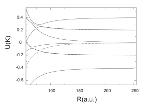
Figure 1: A “slice” through the adiabatic potential energy surfaces for an electric field strength ${\cal E}=10^{4}$ V/cm. In these surfaces $q=-1$, $\omega_{1}=\omega_{2}$, and even (solid line) and odd (dashed line) values of $\langle J\rangle$ are distinguished.

Subdividing the surfaces in this way yields nine surfaces with $q=-1$ and $\omega_{1}=\omega_{2}$, which are of greatest interest here. Slices through these surfaces at a fixed angle $\theta=5^{\circ}$ are shown in Figure 1. Here we take the applied electric field strength to be ${\cal E}=10^{4}$ V/cm. Empirically, we find that surfaces with even values of $\langle J\rangle$ (solid lines) are only weakly coupled to surfaces with odd values of $\langle J\rangle$ (dashed lines). This consideration further reduces the number of surfaces necessary to describe the FL states.

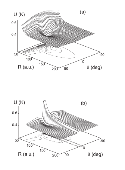
Figure 2: Adiabatic potential energy surfaces corresponding to the highest-lying slice in Fig. 1. Shown are the ${\cal M}=0$ (a) and ${\cal M}=1$ (b) cases.

The FL states are bound states of the highest-lying surface in Figure 1, which is clearly generated by avoided crossings. The complete surface in the $(R,\theta)$ plane is shown in Figure 2 for both the rotationless case ${\cal M}=0$ and a rotating case with ${\cal M}=1$. Addition of the centrifugal energy makes the ${\cal M}=1$ surface substantially more shallow than the ${\cal M}=0$ surface; in fact we find six bound states for ${\cal M}=0$, and only two for ${\cal M}=1$ (see Table I).

${\cal M}$	$v$	Energy (K)
0	0	$0.0282$
0	1	$0.00550$
0	2	$0.000455$
1	0	$0.00545$

Table 1: Binding energies in Kelvin of FL states. Each state is identified by its rotation ${\cal M}$ about the electric field axis, and by a vibrational quantum number $v$. These energies refer to states even under the reflection $\theta\rightarrow\pi-\theta$. Additional states, odd under this symmetry, are separated in energy by less than several $\mu$K from the ones listed.

To gain a better understanding of the nature of the FL states, it is useful to evaluate mean values of the quantum numbers in our basis set. In general, the symmetry-type quantum numbers $x$, $s$, and $\epsilon$ are badly nonconserved, and average to zero. However, the angular momentum quantum numbers $J$ and $K$ typically have well-defined mean values that are useful for interpretation.

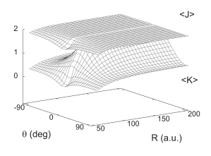
Figure 3: Average values of $J$ and $K$ for the ${\cal M}=0$ potential in Fig.2. Note that the orientation of the axes is different from that in Figs 2 and 4.

Figure 3 shows surface plots of the mean values $\langle J\rangle$ and $\langle K\rangle$ for the FL potential surface (note that the axes are rotated relative to Fig. 2). Near the minima of the potential wells, we find that $\langle J\rangle\approx\langle K\rangle\approx 2$. These values characterize the FL states at large separation $R$. Ref. Schreel presents a simple and useful semiclassical picture of the dipole’s orientation in the OH molecule. In this model the dipole precesses around the molecule’s total angular momentum $\bm{j}$, and on average points along $\bm{j}$ when $\omega>0$, and against $\bm{j}$ when $\omega<0$. Thus when $\langle J\rangle\approx\langle K\rangle\approx 2$ and $\omega_{1}\ \omega_{2}$, as is the case here, the dipole moments are both aligned on average in the same direction, roughly along the intermolecular axis, and hence attract one another.

At smaller values of $R$, $\langle J\rangle$ remains nearly equal to 2, but $\langle K\rangle$ drops all the way to 0. This reflects the influence of the avoided crossings in the surfaces. Again invoking a semicalssical picture, $\langle J\rangle=2$, $\langle K\rangle=0$ implies that the dipole moments are now aligned roughly perpendicular to the intermolecular axis, in a side-by-side orientation where they repel one another. This is the reason the FL state is stable against collapse to smaller $R$.

The avoided crossings that allow FL states to be supported have their origin in the fact the the Stark interaction is diagonal in the laboratory frame (defined by the field axis), whereas the dipolar interaction is diagonal in the rotating frame (defined by the intermolecular axis). Competition between these two symmetries generate the avoided crossings. However, in the limit where $\theta\rightarrow 0$ the two axes coincide and both interactions become diagonal in $K$. In this case the avoided crossings become diabatic crossings, and there is a conical intersection in the surfaces. Our description in terms of adiabatic surfaces is, therefore, incomplete. It is however useful, as we will see in the next section. There may be interesting information on geometrical phases inherent in the FL states; this will be a topic of future study.

III.2 Bound states

To complete a description of the FL states we must understand their motion in $R$ and $\theta$. Each bound state is nearly doubly-degenerate with respect to reflection in the $\theta=\pi/2$ plane. In Figure 4 we present wave function plots of those bound states that have even reflection symmetry, corresponding to the bound states listed in Table I. In this figure, (a-c) refer to the ${\cal M}=0$ case, and (d) to the ${\cal M}=1$ case. for ${\cal M}=0$, it is immediately evident that these states exhibit zero-point motion in the $\theta$ direction, and that excitations are primarily in the $R$ direction. We therefore label the FL states with a vibrational quantum number $v$. For ${\cal M}=1$, a nodal line appears along the $\theta=0$ direction, owing to the centrifugal energy that forces the molecules away from the electric field axis.

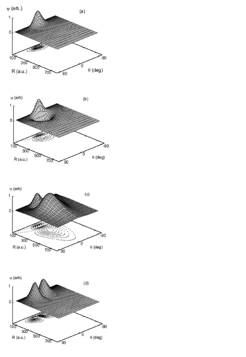
Figure 4: Wave functions of FL states, for the potential surfaces shown in Fig. 2. For ${\cal M}=0$, there are three vibrational states, $v=0$ (a), $v=1$ (b), and $v=2$ (c). For ${\cal M}=1$, there is a single state, with $v=0$ (d).

In realistic laboratory circumstances, the FL states are quasi-stable, being subject to dissociation into free molecules in lower-energy internal states AB1 . Nevertheless, the adiabatic bound states we have identified here correspond to real features of these dissociating states. To show this, we have carried out a complete coupled-channel scattering calculation in a laboratory-frame representation, similar to that in Ref. AB2 , but without including hyperfine structure. We have included partial waves up to $L=16$ to ensure convergence at the several percent level in scattering observables.

We compute the time delay for the scattering process, defined as Fano

$$\tau=2\hbar{d\delta\over dE},$$ (41)

where $\delta$ is the eigenphase sum, i.e., the sum of the inverse tangents of the eigenvalues of the scattering K-matrix. This quantity, plotted in Figure 5, exhibits peaks at energies where resonances occur. There is also a significant background component, arising from threshold effects, but the peaks are nevertheless visible. Also indicated are the binding energies of the FL states as given in Table I. The good agreement between the two calculations suggests that when FL resonances are observed in experiments, the nature of the resonant states will be well-approximated by the wave functions determined above.

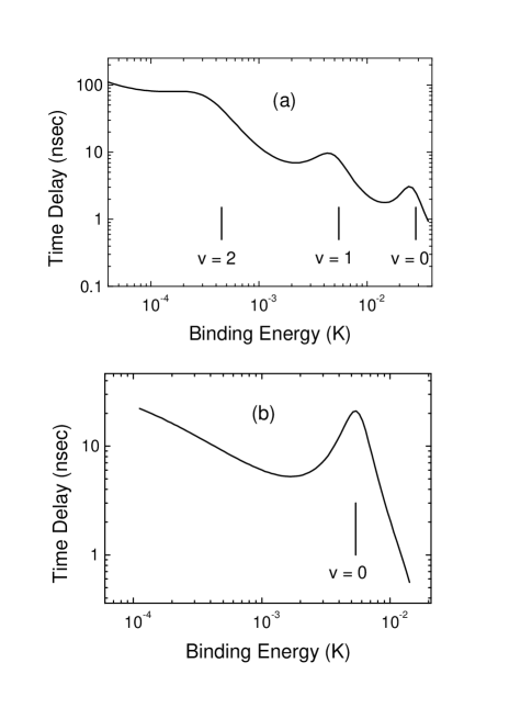
Figure 5: Time delay as defined in Eqn. (22) for the ${\cal M}=0$ (a) and ${\cal M}=1$ (b) FL states. Resonance peaks appear at characteristic energies that correlate well with the binding energies as determined from the FL adiabatic surfaces (vertical lines).

In general, resonances in ultracold polar molecule scattering will come in three varieties. The “true” field-linked states, like the ones that we describe here, are largely independent of physics at small values of $R$. We can verify this assertion by changing the small-$R$ boundary conditions in our multichannel scattering calculation. The positions of the FL resonances do not depend at all on these boundary conditions. However, their lifetimes can fluctuate within a factor of $\sim 2$, since the continuum states into which they can decay do depend on short-range physics.

A second type of FL state appears to have components at both large and small $R$. Examples of these are found for states lying below the middle threshold in Fig. 1. We find that their positions are relatively insensitive to the short-range boundary conditions, but that their lifetimes vary wildly. We refer to these as “quasi-FL” states. Finally a third category of resonance is strongly sensitive to initial conditions, both in position and width. These are resonant states of the short-range interaction, which are expected to be numerous in low-energy molecular collisions Forrey ; AB3 .

IV Outlook

We have left out many details of molecular structure and interactions, in order to emphasize the basic structure of the field-linked states. This structure is remarkably simple, and consists primarily of a pair of molecules in relative vibrational motion along an axis that nearly coincides with the direction of the electric field. The number of FL states is not large, since the forces holding them together are necessarily weak.

Significantly, to adapt this simple picture to a particular molecular species requires only a detailed knowledge of the structure of each molecule separately, plus some information on long-range parameters such as dispersion coefficients. In other words, realistic modeling of experimentally probed FL states can probably be achieved using currently existing information. This is in stark contrast with molecular collisions involving close contact between the molecules, in which case existing potential energy surfaces are likely to be inadequate for to describe collisions at ultralow temperatures.

Appendix A Symmetrized wave functions

To incorporate the effects of symmetrization under the exchange (${\hat{P}}_{12}$) and parity (${\hat{I}}$) operations, we follow the treatment of Alexander and DePristo alexander . To this end it is convenient to relate the Euler angles of each molecule to the electric field axis rather than the intermolecular axis; these Euler angles are denoted $\bm{\hat{e}}^{L}$. The symmetry operations then perform the following functions:

$${\hat{P}}_{12}: \bm{R}\rightarrow-\bm{R}$$

$$\bm{\hat{e}}^{L}_{1}\rightarrow\bm{\hat{e}}^{L}_{2}$$

$$\bm{\hat{e}}^{L}_{2}\rightarrow\bm{\hat{e}}^{L}_{1}.$$

$${\hat{I}}: \bm{R}\rightarrow-\bm{R}$$

$$\bm{\hat{e}}^{L}_{1}\rightarrow{\hat{I}}(\bm{\hat{e}}^{L}_{1})$$

$$\bm{\hat{e}}^{L}_{2}\rightarrow{\hat{I}}(\bm{\hat{e}}^{L}_{2}).$$

The last two lines imply that ${\hat{I}}$ acts on each molecule by inverting the molecule’s coordinates through its own center of mass.

The effect of particle exchange on the internal coordinates is determined by making the explicit rotation to the lab frame:

$${\hat{P}}_{12}\langle\bm{\hat{e}}_{1},\bm{\hat{e}}_{2}|(1,2)JK\rangle$$

$$={\hat{P}}_{12}\sum_{m_{12}}\langle\bm{\hat{e}}^{L}_{1},\bm{\hat{e}}^{L}_{2}|(1,2)Jm_{12}\rangle D^{J}_{m_{12},K}(\phi,\theta,0)$$

$$=\sum_{m_{12}}(-1)^{2j+J}\langle\bm{\hat{e}}^{L}_{1},\bm{\hat{e}}^{L}_{2}|(2,1)Jm_{12}\rangle(-1)^{J}D^{J}_{m_{12},-K}(\phi,\theta,0)$$

$$=(-1)^{2j}\langle\bm{\hat{e}}_{1},\bm{\hat{e}}_{2}|(2,1)J-K\rangle.$$

Here we have used the reflection symmetry of the Wigner $D$ functions,

$$D^{J}_{mK}(\pi+\phi,\pi-\theta,0)=(-1)^{J}D^{J}_{m-K}(\phi,\theta,0)$$

and the usual exchange symmetry of the Clebsch-Gordan coefficients. Similarly the relative wave functions transform as

$${\hat{P}}_{12}\left[\exp(i{\cal M}\phi)F^{\cal M}_{(1,2)JK}(R,\theta)\right]$$

$$\;\;\;\;=(-1)^{\cal M}\exp(i{\cal M}\phi)F^{\cal M}_{(1,2)JK}(R,\pi-\theta).$$

An appropriately symmetrized basis for exchange is therefore given by Eqn. (II.1), where

$$F^{{\cal M},s}_{(1,2)JK}={1\over 2}$$

$$\;\;\;\;\times\left[F^{\cal M}_{(1,2)JK}(R,\theta)+s(-1)^{\cal M}F^{\cal M}_{(1,2)JK}(R,\pi-\theta)\right],$$

$$|(1,2)JK\rangle_{x}={1\over\sqrt{2(1+\delta_{12}\delta_{K0})}}$$

$$\;\;\;\;\times\left[|(1,2)JK\rangle+x(-1)^{2j}|(2,1)J-K\rangle\right],$$

with $sx=\pm 1$ for bosons/fermions.

These basis functions can in turn be assembled into parity eigenfunctions. Note that ${\hat{I}}$ has the same effect on the relative coordinates as does ${\hat{P}}_{12}$, so that $e^{i{\cal M}\phi}F^{{\cal M},s}_{(1,2)JK}$ is already a parity eigenstate with eigenvalue $s$. Denoting the parity of the total wave function by $\epsilon$, the parity of the relative wavefunctions should be $p=\epsilon s$, or $p=q(-1)^{K}$ in terms of our quantum number $q$ defined in Eqn.(6). This definition seems (and is) completely arbitrary; it is justified by explicitly working out the matrix elements for the Stark and dipole-dipole interactions, and finding that both conserve the value of $q$.

The influence of ${\hat{I}}$ on each molecule is to reverse its direction of rotation about its own axis, and to introduce a phase Singer :

$${\hat{I}}\langle\bm{\hat{e}}^{L}|j,m,\omega\rangle=(-1)^{j-s}\langle\bm{\hat{e}}^{L}|jm-\omega\rangle.$$

Because the phase factor is the same for each molecule, the action of ${\hat{I}}$ on the molecule pair is, by arguments similar to those above,

$${\hat{I}}\langle\bm{\hat{e}}_{1}\bm{\hat{e}}_{2}|(1,2)JK\rangle=(-1)^{J}\langle\bm{\hat{e}}_{1}\bm{\hat{e}}_{2}|(-1,-2)J-K\rangle,$$

where the notation $(1,2)\rightarrow(-1,-2)$ implies $(j_{1},\omega_{1},j_{2},\omega_{2})\rightarrow$ $(j_{1},-\omega_{1},j_{2},-\omega_{2})$. The symmetrized internal basis function is then

$$|(1,2)JK\rangle_{x,q}=$$

$$\;\;\;\;{1\over\sqrt{2}}\left[|(1,2)JK\rangle_{x}+q(-1)^{J+K}|(-1,-2)J-K\rangle_{x}\right].$$

Appendix B Conservation of $q$

It is straightforward (if somewhat tedious) to write the symmetrized matrix elements for different contributions to the Hamiltonian, in terms of the unsymmetrized basis. We present here some of the key results, which rely mostly on the symmetry properties of the angular momentum recoupling coefficients, as described in Brink and Satchler BS .

Dipolar interaction. In Eqn. (II.2.2), the 9-$j$ symbol must be invariant under exchanging its second and third rows, yet this operation introduces a phase shift $(-1)^{J+2+J^{\prime}}$. Therefore, we must have $J+J^{\prime}=$ even, and the matrix element (II.2.2) is invariant under the substitution $(1,2)\rightarrow(2,1)$, $K\rightarrow-K$. In the symmetrized basis it reads

$${}_{x}\langle(1,2)JK|V_{\mu\mu}|(1^{\prime},2^{\prime})J^{\prime}K^{\prime}\rangle_{x}=$$

$$\;\;\;\;\left({1+xx^{\prime}\over 2}\right){1\over\sqrt{(1+\delta_{12}\delta_{K0})(1+\delta_{1^{\prime}2^{\prime}}\delta_{K^{\prime}0})}}$$

$$\;\;\;\;\times\biggl{[}\langle(1,2)JK|V_{\mu\mu}|(1^{\prime},2^{\prime})J^{\prime}K^{\prime}\rangle$$

$$\;\;\;\;\;\;+x^{\prime}(-1)^{2j}\langle(1,2)JK|V_{\mu\mu}|(2^{\prime},1^{\prime})J^{\prime}-K^{\prime}\rangle\biggr{]}.$$

Thus the exchange quantum number $x$ is explicitly conserved. Similarly, the matrix elements are invariant under simultaneously reversing the signs of all $\omega$’s and $K$, whereby

$${}_{x,q}\langle(1,2)JK|V_{\mu\mu}|(1^{\prime},2^{\prime})J^{\prime}K^{\prime}\rangle_{x^{\prime},q^{\prime}}=$$

$$\;\;\;\;\biggl{(}{1+qq^{\prime}(-1)^{K+K^{\prime}}\over 2}\biggr{)}$$

$$\;\;\;\;\times\biggl{[}_{x}\langle(1,2)JK|V_{\mu\mu}|(1^{\prime},2^{\prime})J^{\prime}K^{\prime}\rangle_{x^{\prime}}$$

$$\;\;\;\;\;\;\;\;+q^{\prime}(-1)^{K^{\prime}}\;_{x^{\prime}}\langle(1,2)JK|V_{\mu\mu}|(-1^{\prime},-2^{\prime})J^{\prime}-K^{\prime}\rangle_{x^{\prime}}\biggr{]}.$$

Because $K=K^{\prime}$ for the dipolar interaction, this implies in turn that $q$ is conserved. The matrix derivation of symmetrized matrix elements for the lambda-doubling is exactly the same, and this interaction also conserves $q$.

Stark interaction. Symmetrized matrix elements of the Stark Hamiltonian (II.2.1) are slightly more complicated, since reversing the sign of $K$ also affects the Wigner $d$-function. Exploiting symmetries of the $d$ functions yields

$${}_{x}\langle(1,2)JK|H^{S}|(1^{\prime},2^{\prime})J^{\prime}K^{\prime}\rangle_{x^{\prime}}=$$

$$\;\;\;\;\biggl{(}{1-xx^{\prime}(-1)^{K+K^{\prime}}\over 2}\biggr{)}{1\over\sqrt{(1+\delta_{12}\delta_{K0})(1+\delta_{1^{\prime}2^{\prime}}\delta_{K^{\prime}0})}}$$

$$\times\Biggl{[}\langle(1,2)JK|H^{S}|(1^{\prime},2^{\prime})J^{\prime}K^{\prime}\rangle d^{1}_{0,K^{\prime}-K}(\theta)$$

$$\;\;\;\;+x^{\prime}(-1)^{2j}\langle(1,2)JK|H^{S}|(2^{\prime},1^{\prime})J^{\prime}-K^{\prime}\rangle d^{1}_{0,K^{\prime}-K}(\theta)\Biggr{]}.$$

In general, neither $x$, nor $K$, nor the product $x(-1)^{K}$, is conserved by this part of the Hamiltonian. However, the matrix elements in the basis (7) become

$${}_{x,q}\langle(1,2)JK|H^{S}|(1^{\prime},2^{\prime})J^{\prime}K^{\prime}\rangle_{x^{\prime},q^{\prime}}=\biggl{(}{1+qq^{\prime}\over 2}\biggr{)}$$

$$\times\biggl{[}_{x}\langle(1,2)JK|H^{S}|(1^{\prime},2^{\prime})J^{\prime}K^{\prime}\rangle_{x^{\prime}}$$

$$\;\;\;\;\;+q^{\prime}(-1)^{K^{\prime}}\;_{x^{\prime}}\langle(1,2)JK|H^{S}|(-1^{\prime},-2^{\prime})J^{\prime}-K^{\prime}\rangle_{x^{\prime}}\biggr{]},$$

illustrating the conservation of $q$.

Centrifugal energy. Symmetrized over $x$, the centrifugal energy reads

$${}_{x}<(1,2)JK|V^{cent}|(1^{\prime},2^{\prime})J^{\prime}K^{\prime}>_{x^{\prime}}=\frac{\hbar^{2}}{2mR^{2}}\delta_{J,J^{\prime}}\times\Biggl{(}{1+xx^{\prime}\over 2}\Biggr{)}\Biggl{(}{1\over\sqrt{4(1+\delta_{1,2}\delta_{K,0})(1+\delta_{1^{\prime},2^{\prime}}\delta_{K^{\prime},0})}}\Biggr{)}$$

$$\times\Biggl{[}\biggl{(}\hat{A}_{0}(K)\delta_{K,K^{\prime}}+\hat{A}_{-1}(K)\delta_{K,K^{\prime}+1}+\hat{A}_{+1}(K)\delta_{K,K^{\prime}-1}\biggr{)}\delta_{1,1^{\prime}}\delta_{2,2^{\prime}}$$ (42)

$$+x^{\prime}\biggl{(}\hat{A}_{0}(K)\delta_{-K,K^{\prime}}+\hat{A}_{-1}(K)\delta_{-K,K^{\prime}+1}+\hat{A}_{+1}(K)\delta_{-K,K^{\prime}-1}\biggr{)}\delta_{1,2^{\prime}}\delta_{2,1^{\prime}}\Biggr{]}$$

From this point, translation into the $x,q$ symmetrized basis is trivial. In general, $q$ is not conserved by the Coriolis terms that change $K$, but in the present treatment these terms are ignored.

References

- (1) For a recent review, see H. L. Bethlem and G. Meijer, Int. Rev. Phys. Chem. 22, 73 (2003).
- (2) J. D. Weinstein, R. deCarvalho, T. Guillet, B. Friedrich, and J. M. Doyle, Nature (London) 395, 148 (1998).
- (3) D. Egorov, J. D. Weinstein, D. Patterson, B. Friedrich, and J. M. Doyle, Phys. Rev. A 63, 030501 (2001).
- (4) H. L. Bethlem, G. Berden, F. M. H. Crompvoets, R. T. Jongma, A. J. A. van Roij, and G. Meijer, Nature (London) 406, 491 (2000).
- (5) H. L. Bethlem, F. M. H. Crompvoets, R. T. Jongma, S. Y. T. van der Meerakker, and G. Meijer, Phys. Rev. A 65, 053416 (2002).
- (6) J. R. Bochinksi, E. R. Hudson, H. J. Lewandowski, J. Ye, and G. Meijer, LANL preprint server physics/0306062 (2003).
- (7) A. J. Kerman, J. M. Sage, S. Sainis, D. DeMille, and T. Bergeman, LANL preprint server physics/0308020 (2003).
- (8) S. A. Rangwala, T. Junglen, T. Rieger, P. W. H. Pinske, and G. Rempe, Phys. Rev. A 67, 043406 (2003).
- (9) N. E. Shafer-Ray, K. A. Milton, B. R. Furneaux, E. R. I. Abraham, G. R. Kalbfleisch, Phys. Rev. A 67, 045401 (2003).
- (10) N. Balakrishnan and A. Dalgarno, Chem. Phys. Lett. 341, 652 (2001).
- (11) L. Santos, G. V. Shlyapnikov, P. Zoller, and M. Lewenstein, Phys. Rev. Lett. 85, 1791 (2001).
- (12) P. M. Lushnikov, Phys. Rev. A 66 051601 (2002).
- (13) A. Derevianko, Phys. Rev. A 67, 033607 (2003).
- (14) M. A. Baranov, M. S. Mar’enko, V. S. Rychkov and G. V. Shlyapnikov, Phys. Rev. A 66, 013606 (2002) .
- (15) K. Góral, M. Brewczyk, and K. Rza̧żewski, Phys. Rev. A 67, 025601 (2003).
- (16) D. DeMille, Phys. Rev. Lett. 88, 067901 (2002).
- (17) A. V. Avdeenkov and J. L. Bohn, Phys. Rev. Lett. 90, 043006 (2003).
- (18) A. V. Avdeenkov and J. L. Bohn, Phys. Rev. A 66, 052718 (2002)
- (19) A. Derevianko, S. G. Porsev, S. Kotochigova, E. Tiesinga, and P. S. Julienne, Phys. Rev. Lett. 90, 063002 (2003)
- (20) R. Santra and C. H. Greene, Phys. Rev. A 67, 062713 (2003).
- (21) V. Kokoouline, R. Santra, and C. H. Greene, Phys. Rev. Lett. 90, 253201 (2003).
- (22) J. A. Coxon, Can. J. Phys. 58, 933 (1980).
- (23) K. Schreel and J. J. ter Muelen, J. Phys. Chem. A 101, 7639 (1997).
- (24) D. M. Brink and G. R. Satchler, Angular Momentum (Third edition, Oxford, 1993).
- (25) J. M. Launay, J.Phys.B, 9, 1823 (1976)
- (26) D. A. Varshalovich, A. N. Moskalev, and V. K. Khersonskii, Quantum Theory of Angular Momentum (World Scientific, 1988).
- (27) M. H. Alexander, A. E. DePristo, J.Chem. Phys. 66, 2166 (1977)
- (28) Singer, Freed, and Band, J. Chem. Phys. 79, 6060 (1983).
- (29) U. Fano and A. R. P. Rau, Atomic Collisions and Spectra (Orlando, Academic Press, 1986, p. 69).
- (30) R. C. Forrey, N. Balakrishnan, V. Kharchenko, and A. Dalgarno, Phys. Rev. A 58, R2645 (1998).
- (31) J. L. Bohn, A. V. Avdeenkov, and M. P. Deskevich, Phys. Rev. Lett. 89, 203202 (2002).