Wave Mechanics of a Two Wire Atomic Beamsplitter

Abstract

We consider the problem of an atomic beam propagating quantum mechanically through an atom beam splitter. Casting the problem in an adiabatic representation (in the spirit of the Born-Oppenheimer approximation in molecular physics) sheds light on explicit effects due to non-adiabatic passage of the atoms through the splitter region. We are thus able to probe the fully three dimensional structure of the beam splitter, gathering quantitative information about mode-mixing, splitting ratios,and reflection and transmission probabilities.

I Introduction

Continuing advances in the production and manipulation of atomic Bose-Einstein condensates (BEC’s) are tending toward novel applications in interferometry. BEC’s can now be produced in situ on surfaces Hansel ; Kasper ; Ott , making them ready for loading into “interferometer-on-a-chip” micro-structures. Being in close proximity to the chip, the atoms are subject to control via magnetic fields generated by wires on the chip. Because of their coherence and greater brightness, Bose- condensed atoms are expected to improve upon previous accomplishments with thermal atoms, such as neutral atom guiding, Schmiedmayer ; muller ; dekker ; Sauer ; Engels , switching muller2 , and multi-mode beamsplitting Cassettari ; muller3 . Studies of propagation of BEC’s through waveguide structures are also underway leanhardt .

While the BEC is created in its lowest transverse mode in the guiding potential, keeping it in this mode as it travels through the chip remains remains a significant technical challenge. For example, it appears that inhomogeneities in the guiding wires produce field fluctuations that can break up the condensate wave function leanhardt ; schwindt . Additionally, the very act of splitting a condensate into two paths implies a transverse pull on the condensate that can excite higher modes. Ideally, the condensate propagates sufficiently slowly that, once in its lowest mode, it follows adiabatically into the lowest mode of the split condensate. The criterion for this to happen, roughly, is that the condensate velocity in the direction of motion be less than $L\omega$, where $L$ is a characteristic length scale over which the beam is split, and $\omega$ is a characteristic frequency of transverse oscillation in the guiding potential. Reference zozulya has verified this conclusion numerically, in a two-dimensional model that varies the transverse potential in time, at a rate equivalent to the passage of the moving condensate through a beam splitter. Populating higher modes can reduce fringe contrast, thus spoiling the operation of an interferometer. Diffraction has also been pointed out to have negative effects on guiding in general Jaask .

Moving too slowly through the beam splitter is, however, potentially dangerous because of threshold scattering behavior in a varying potential. In one dimension, a wave incident on a scattering potential is reflected with unit probability in the limit of zero collision energy sadeghpour . This same kind of “quantum reflection” will be generically present in beam splitters as well, where scattering can occur from changes in the transverse potential as the longitudinal coordinate varies. Reflection upon entering the beam splitter region can prove devastating for potential applications such as a Sagnac interferometer.

Both aspects of instability in an atom interferometer can be expressed in terms of quantum mechanical scattering theory of the atoms from the guiding potential. Specifically, a condensate entering a beam splitter in arm $a$ and in transverse mode $m$ possesses a scattering amplitude $S_{am,a^{\prime}m^{\prime}}$ for exiting in arm $a^{\prime}$ in mode $m^{\prime}$. In this paper we therefore cast the general problem of beam splitting in terms of scattering theory. For the time being we restrict our attention to the linear scattering problem, and therefore implicitly consider the regime of weak inter-atomic interactions. This is suitable, since the basic question we raise is the effect of wave mechanical propagation on the atoms. Note that the weakly interacting atom limit is achieved with small atom number, in which case number fluctuations may be problematic zozulya2 . Alternatively, this limit is reached at low atom density, which is achieved for a BEC that has expanded longitudinally for some time before entering the beam splitter region.

Restricting our attention to the linear Schrödinger equation opens up a host of powerful theoretical tools that have been developed in the context of atomic scattering. In the present instance, given the dominant role of non-adiabatic effects, the tool of most use is the adiabatic representation. This is analogous to the Born-Oppenheimer approximation in molecular physics Levine . Specifically, we freeze the value of the longitudinal coordinate $z$ and solve the remaining 2-dimensional Schrödinger equation in $x$-$y$. The resulting $z$-dependent energy spectrum represents a set of potential curves for following the remaining motion in $z$. This general approach has been applied previously to a model situation in which the transverse potential is gently contracted or expanded Jaask ; Jaask2 ; here we extend it to realistic waveguide geometries.

This representation has obvious appeal for the problem at hand, since in this level of approximation it is assumed that the atoms move infinitely slowly through the beam splitter. It is, however, an exact representation of scattering theory, and the leftover non-adiabatic corrections, arising from finite propagation velocity, can be explicitly incorporated. We will see that non-adiabatic effects have a strong influence on beamsplitters based on experimentally realistic parameters. The effects of excitation of higher transverse modes and of reflection from the beam splitter therefore have a fairly simple interpretation in these explicit nonadiabticites. In addition, the successive solution of a set of two-dimensional problems in transverse coordinates $x-y$, followed by a coupled-channel calculation in $z$, is less numerically intensive than than determining the full 3-dimensional solution all at once. Indeed, this is why adiabatic representations have found widespread use in chemical physics. Larger problems, more closely resembling experimental beam splitters, can therefore be handled. This paper is organized as follows: In section II we introduce the model, describing how the beamsplitter works in general terms and outlining the theoretical methods used in the paper, introducing the main ideas about the adiabatic formalism. In section III we present the results obtained from our study, with a focus on the description of the theory itself, and how its different components relate to the physics of the problem.

II Model

The salient characteristics of a two wire atomic beam-splitter can be realized in the following way: a guiding potential is generated by the magnetic field due to two parallel current carrying wires and an additional bias field perpendicular to them. By suitably decreasing the bias field or the distance between the wires, it is possible to decrease the separation between two minima, and thus increase the probability for the atoms to tunnel from one to another.

II.1 The Beam Splitting Potential.

We start by considering the magnetic field generated by two infinitely long parallel wires lying on a substrate, each carrying a current $I$ in the $\hat{z}$ direction. Defining the plane of the substrate as the $x-z$ plane, we let the $z$ axis lie exactly between the wires, and let $y$ axis point to the region above the substrate. hinds

We then proceed with the addition of two bias fields, one in the $\hat{z}$ direction, $B_{bz}$, and one in the $\hat{x}$ direction, $B_{bx}$. The first of the two is put in place in order to avoid regions of exactly zero field, where Majorana transitions would cause arbitrary spin flips, and therefore loss of atoms from the guide. The second of the two fields, when added vectorially to the field generated by the wires, generates regions of minimum potential in the $x-z$ plane. In particular, for $B_{bx}^{0}=\mu_{0}I/2\pi d$ ,where $\mu_{0}$ is the permeability of free space, and $d$ is the separation between the wires, there exists a single potential minimum located on the y axis a distance $y_{0}=d$ above the wires.

Furthermore, for $B_{bx}<B_{bx}^{0}$ two minima are generated on the y axis, one above and one below $y_{0}$, and for $B_{bx}>B_{bx}^{0}$, two minima are again generated above the substrate, but this time they are displaced symmetrically to the left and the right of the $y-z$ plane. It is this latter regime that we use to generate a beam splitter, letting the wires be fixed, and changing the transverse bias field $B_{bx}$ as a function of $z$ from $B_{max}$ to $B_{min}$ and back, such that $B_{max}>B_{min}>B_{bx}^{0}$.

The magnetic field produced by such configuration is therefore zozulya2 ; hinds

$$B_{x} =\frac{\mu_{0}I}{2\pi}\left[\frac{-y}{(x-d)^{2}+y^{2}}+\frac{-y}{(x+d)^{2}+y^{2}}\right]+B_{bx}(z)$$

$$B_{y} =\frac{\mu_{0}I}{2\pi}\left[\frac{x-d}{(x-d)^{2}+y^{2}}+\frac{x+d}{(x+d)^{2}+y^{2}}\right]$$

$$B_{z} =B_{bz}$$

and the consequent potential experienced by the atoms is

$$V=g_{F}\mu_{B}m_{F}|\mathbf{B}|,$$ (2)

where $\mu_{B}$ is the Bohr magneton, $g_{F}$ is the Landé factor, $m_{F}$ is the total angular momentum projection quantum number, and the atoms’ spin is aligned with the field at every point in space. An example of a guiding potential is illustrated in Fig 1.

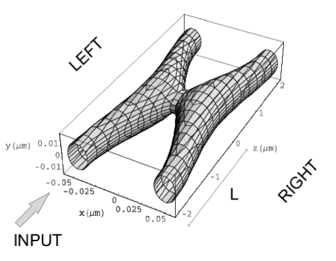
Figure 1: Constant Energy surface representing the potential in Eq.(2). The parameters chosen for this plot are $d=0.1\mu m$, $B_{min}=21.3G$, $B_{max}=22.5G$, $B_{bz}=1.0G$, $L=20\mu m$. The surface contour is drawn at the energy of the lowest mode of the input arm of the beamsplitter, and we define “left” and “right” arms for labeling convenience.

The adjustable experimental parameters are therefore the current in the wires $I$, the values of the bias fields $B_{max}$ , $B_{min}$ and $B_{bz}$, and the distance $d$ between the wires. Throughout this work we choose, for concreteness, $d=0.1\mu m$, $B_{min}=21.3G$, $B_{max}=22.5G$, $B_{bz}=1.0G$, $L=20\mu m$, and we let $B_{bx}(z)$ be a fourth order polynomial in z, such that it has zero derivative at the center ( $z=0$) and edges ($z=\pm L$) of the beam splitter. Also we will only consider cases in which $B_{bx}(z)$ reaches its minimum value at $z=0$ only, avoiding the characterization of the trivial evolution of the wave function at a constant field. In particular we will consider the following form for the variation of the transverse bias field:

$$B_{bx}(z)=B_{mim}+(B_{min}-B_{max})\left[2(x/L)^{2}-(x/L)^{4}\right]$$ (3)

Varying $L$ will therefore adjust the adiabaticity of the beamsplitter, whose effects we will study in section (III B)

II.2 Waveguides as a Scattering Problem

Because we are going to treat the beamsplitter as a scattering problem, we will begin by offering a quick review of scattering theory; in particular we will reproduce the basic formulation of the adiabatic treatment of the scattering problem.

Scattering theory is fundamentally based on the superposition principle, which constrains us to the solution of the linear Schrödinger equation. This limit is nonetheless justifiable in light of the known problems caused by the interaction between atoms, such as the wave function recombination instabilities described in Ref.zozulya3 .

The separation between the guides at the input and output ports of the beam-splitter is sufficiently great that no tunneling is possible between the guides within the time frame of the experiment. The problem is thus divided into two separate regions. We will refer to the region $|z|<L$ as the scattering region. This is the inner region containing the active part of the beam-splitter, where all the coupling between the modes takes place. In the outer region, defined by $|z|>L$,the potential has translational symmetry in $z$. Solutions to the Schrödinger equation in the outer region are therefore trivially found to be products of transverse modes and longitudinal plane-wave solutions. The problem is thus reduced to finding solutions inside the scattering region, and match them to the solutions outside to find solutions to the global problem. Once these solutions are found it is then possible to generate the S-matrix for the system.

Moreover, since we are matching at the boundary of the scattering region the only information we need is the value of the wave function and its derivative at the boundary, and nowhere else. In particular we need to compute the quantity

$$b=-\left.\frac{1}{\Psi(\mathbf{r})}\frac{\partial\Psi(\mathbf{r})}{\partial n}\right|_{\Sigma},$$ (4)

defined as the logarithmic derivative, where $\Sigma$ is the boundary of the scattering region, $n$ is the outward normal to the surface $\Sigma$, and $\Psi$ is the wave function in the inner region. Because the wave function must vanish in the limit of large $|x|$ or $|y|$, the surface $\Sigma$ consists, for us, of the two planes $z=\pm L$. To find solutions inside the box we used the R-matrix method, formulated in the adiabatic representation. A derivation of this method follows.

II.3 The Adiabatic representation

We start by writing the Shrödinger equation

$$-\frac{\hbar^{2}}{2m}\frac{\partial^{2}}{\partial z^{2}}\Psi(x,y,z)+\left[-\frac{\hbar^{2}}{2m}\nabla_{x,y}^{2}+V(x,y,z)\right]\Psi(x,y,z)=E\Psi(x,y,z),$$ (5)

with $V(x,y,z)$ as defined in Eq.(2). If atoms in the guide were moving infinitely slowly , i.e. adiabatically, then the wave function would be well represented by the basis set $\phi_{i}(x,y;z)$ with eigenvalues $U_{i}(z)$, defined as solutions to the equation

$$\left[-\frac{\hbar^{2}}{2m}\nabla_{x,y}^{2}+V(x,y;z)\right]\phi_{i}(x,y;z)=U(z)\phi_{i}(x,y;z).$$ (6)

As in the Born-Oppenheimer approximation, the quantities $U_{i}(z)$ serve as effective potentials for the subsequent motion in $z$. To recover the effect of finite velocity in $z$, it would be appropriate to expand the wave function in terms of the adiabatic basis in the following way:

$$\Psi(x,y,z)=\sum_{j}F_{j}(z)\phi_{j}(x,y;z),$$ (7)

where the $z$ dependence of the coefficient $F_{i}(z)$ is necessary in order to restore the motion in the $z$ coordinate. We should note that the above defined basis functions depend only parametrically on $z$, and they are normalized in the following way:

$$\int\phi_{i}(x,y;z)\phi_{j}(x,y;z)dxdy=\delta_{i,j}.$$ (8)

This normalization implies that all transverse functions must vanish as $x,y\rightarrow\infty$, and therefore defines the effective boundary of the scattering region as $z=\pm L$.

Having defined the basis set we proceed to insert Eqn. (7) into Eqn. (5), and subsequently project the resulting equation onto $\phi_{i}(x,y;z)$, to obtain the set of coupled equations

$$-\frac{\hbar^{2}}{2m}\left[\frac{\partial^{2}}{\partial z^{2}}F_{i}(z)+2\sum_{j}P_{ij}\frac{\partial}{\partial z}F_{j}(z)+\sum_{j}Q_{ij}F_{j}(z)\right]+U_{i}(z)F_{i}(z)=EF_{i}(z)$$ (9)

where we have defined, as conventional,

$$P_{ij}= \left<\phi_{i}(x,y;z)\left|\frac{\partial}{\partial z}\phi_{j}(x,y;z)\right>\right.$$ (10)

$$Q_{ij}= \left<\phi_{i}(x,y;z)\left|\frac{\partial^{2}}{\partial z^{2}}\phi_{j}(x,y;z)\right>.\right.$$ (11)

$P$ and $Q$ are operators of momentum-like and kinetic energy-like quantities, and thus reflect the influence of finite propagation velocity in $z$. Notice that $P$ and $Q$ vanish by construction in the outer region.

We have thus cast the original 3-dimensional problem into a collection of 2-dimensional problems to find $\phi_{i}(x,y;z)$ and $U_{i}(z)$, and a 1-dimensional coupled channel problem to find $F_{i}(z)$. The advantages of this shift in paradigm are twofold: on the one hand, a very complicated and computationally lengthy problem is turned into a simpler and computationally manageable problem; On the other hand, the adiabatic approach lends itself very naturally to approximations and qualitative understanding of the underlying physics.

II.4 The R-Matrix Method

As mentioned earlier, solving the scattering problem implies finding the logarithmic derivative $b$ as defined in Eq.(4). In atomic structure physics, there is a well known variational principle for the logarithmic derivative, which follows rather simply from the Schrödinger equation greene :

$$b=\frac{\int_{\Omega}\left[\vec{\nabla}\Psi^{*}\cdot\vec{\nabla}\Psi+\frac{2m}{\hbar^{2}}\Psi^{*}(V-E)\Psi\right]}{\int_{\Sigma}\Psi^{*}\Psi},$$ (12)

where $\int_{\Omega}$ denotes an integral over the volume of the scattering region, while $V$ is the scattering potential, and $\int_{\Sigma}$ is a surface integral over the surface bounding the scattering region.

The typical approach to the problem, at this point is to expand the wave function in a complete set of basis functions ${Y_{k}}$, to get $\Psi(x,y,z)=\sum_{k}C_{k}Y_{k}(x,y,z)$, and take matrix elements of the operators in Eqn. (12) with respect to such basis, to obtain the following generalized eigenvalue problemgreene :

$$\hat{\Gamma}\vec{C}=b\hat{\Lambda}\vec{C},$$ (13)

where

$$\Gamma_{ij} = \int_{\Omega}\left[\vec{\nabla}Y_{i}^{*}\cdot\vec{\nabla}Y_{j}+\frac{2m}{\hbar^{2}}Y^{*}_{i}(V-E)Y_{j}\right]$$ (14)

$$\Lambda_{ij} = \int_{\Sigma}Y_{i}^{*}Y_{j}.$$ (15)

This is the form that the eigenchannel R-matrix takes in a diabatic representation.

The solutions of the eigenvalue problem consists of a set of eigenvectors $C^{\sigma}$, and a set of eigenvalues $b^{\sigma}$, representing the logarithmic derivatives of the functions $\Psi^{\sigma}=\sum_{k}C_{k}^{\sigma}Y_{k}$. The newly introduced index $\sigma$ refers to the different possible internal states of the system, called R-matrix eigenchannels. The concept of eigenchannel in scattering theory can be understood by analogy with the concept of eigenstate in bound state problems. In fact, just like the energy variational principle leads to an eigenvalue problem for bound state eigenfunction and corresponding energies, the variational principle in Eq.(12) leads to a set of eigenchannels, with corresponding eigen-logarithmic derivatives.

As we mentioned earlier, we plan to work using the adiabatic basis defined in Eq.(7), so we expand Eq.(12) in terms of this set, and obtain the following variational principle:

$$b=\frac{\sum_{ij}\int dz\left[\left\{\frac{\partial}{\partial z}F_{i}^{*}\frac{\partial}{\partial z}F_{j}+\frac{2m}{\hbar^{2}}F_{i}^{*}(U_{i}(z)-E)F_{j}\right\}\delta_{ij}+2F_{i}^{*}P_{ij}\frac{\partial}{\partial z}F_{j}+F_{i}^{*}Q_{ij}F_{j}\right]}{|F_{i}(\Sigma)|^{2}}.$$ (16)

Since the adiabatic basis only defines motion in the transverse coordinates, it remains to expand the longitudinal functions $F_{i}(z)$ with an arbitrary set of $z$ dependent functions, in our particular case we chose basis-splines, in the form $F_{i}(z)=\sum_{k}c_{ik}y_{k}^{i}(z)$. We can now write the adiabatic equivalent to Eq.(13).

In order to simplify the notation, we combine the indices $i,k$ into the index $\alpha$, so that $c_{\alpha}$ becomes a vector, and we write

$$\hat{\Gamma}^{a}\vec{c}=b\hat{\Lambda}^{a}\vec{c},$$ (17)

where

$$\Gamma^{a}_{\alpha\beta} = \int dz\left[\left\{\frac{\partial}{\partial z}y_{\alpha}^{*}\frac{\partial}{\partial z}y_{\beta}+\frac{2m}{\hbar^{2}}y_{\alpha}^{*}(U_{i}(z)-E)y_{\beta}\right\}\delta_{ij}+y_{\alpha}^{*}P_{ij}\frac{\partial}{\partial z}y_{\beta}+\frac{\partial}{\partial z}y_{\alpha}^{*}P_{ji}y_{\beta}+y_{\alpha}^{*}Q_{ij}y_{\beta}\right]$$

$$\Lambda^{a}_{\alpha\beta} = y_{\alpha}^{*}(\Sigma)y_{\beta}(\Sigma)\delta_{ij}.$$ (18)

In the above equations we have written the P-matrix portion of Eq.(16) in an Hermitian form by integrating by parts, and setting the resulting surface integral to zero, using the fact that by definition all couplings $P,Q$ must vanish outside the scattering region.

II.5 The Outer Region: Matching and Physical Consideration

Having solved Eq.(17), one obtains a set of eigenvalues $b^{\sigma}$, and a set of eigenvectors $\vec{c^{\sigma}}$. It therefore follows that on the boundaries $\Sigma$ of the scattering region we can connect the inner and outer solutions by:

$$\Psi^{\sigma}(x,y,\Sigma)=\sum_{j}F_{j}^{\sigma}(\Sigma)\phi_{j}(x,y,\Sigma)=\sum_{\alpha}c_{\alpha}^{\sigma}y_{\alpha}(\Sigma)\phi_{j}(x,y,\Sigma)$$

$$=\sum_{\alpha}\phi_{j}(x,y,\Sigma)*\left(A_{j}^{\sigma}\frac{e^{-ik_{j}\Sigma}}{\sqrt{2|k_{i}|}}+B_{j}^{\sigma}\frac{e^{ik_{j}\Sigma}}{\sqrt{2|k_{i}|}}\right)$$

(19)

where $k_{i}=\sqrt{2m(E-U_{i}(\Sigma))}$ is real for $E>U_{i}(\Sigma)$, and imaginary for $E<U_{i}(\Sigma)$, and $\Sigma=\pm L$. At a particular incoming energy, we define a channel with real $k_{i}$ to be “open” (meaning energetically available) an channel with imaginary $k_{i}$ to be “closed”. If a channel $i$ is closed we set $A_{j}^{\sigma}=0$, to avoid unphysical divergences. A similar argument is valid for the derivative of the wave function:

$$\frac{\partial}{\partial\Sigma}\Psi^{\sigma}(x,y,\Sigma)=-b^{\sigma}\Psi^{\sigma}(x,y,\Sigma)$$

(20)

Eqs(19,20), together with the orthonormality of the set ${\phi_{i}}$, and the assumption of unit incoming flux, imply that $F_{j}^{\sigma}(\Sigma)$ and its derivatives can be written as a linear combination of the form:

$$\left\{\begin{array}[]{rl}F_{i}^{\sigma}(\Sigma)&=\left[\delta_{ij}\frac{e^{-ik_{i}\Sigma}}{\sqrt{2|k_{i}|}}-S_{ij}\frac{e^{ik_{i}\Sigma}}{\sqrt{2|k_{i}|}}\right]N_{j}^{\sigma}\\ \\ b^{\sigma}F_{i}^{\sigma}(\Sigma)&=-\left[\delta_{ij}\frac{ike^{-ik_{i}\Sigma}}{\sqrt{2|k_{i}|}}-S_{ij}\frac{-ike^{ik_{i}\Sigma}}{\sqrt{2|k_{i}|}}\right]N_{j}^{\sigma}\\ \end{array}\right.$$ (24)

The quantity $N_{i}^{\sigma}$ is a factor which serves to connect the normalizations of the two equations. On the other hand $S_{ij}$ is the scattering matrix of the system (often referred to as S-matrix), and it represents the probability amplitude to enter the beam splitter in channel $j$, and exit it in channel $i$, or vice versa, since $S$ is Hermitian due to time reversal symmetry.

Moreover, since the equation is true on the whole of the boundary, the channel index describes the probability amplitude for the atom to be found at either end of the beam splitter (in fact at any particular arm of the beam splitter), in some particular mode. This allows us to calculate mode mixing, as well as reflection and transmission amplitudes.The above system of equations can be solved for the unknowns $S_{ij}$ and $N^{\sigma}_{j}$.

II.6 Solving the Equations: Considerations on Numerical and Mathematical Details

The numerical problem consists of two main parts. The first is to find the transverse eigenmodes $\phi_{i}(x,y;z)$. This is accomplished by solving Eq.(6) at various values of $z$ in such a way that the adiabatic curves $U_{i}(z)$ may be interpolated easily. We accomplish this task by generating a Hamiltonian matrix, again using b-splines as a basis set, and diagonalizing it at various values of $z$.

Furthermore one needs to evaluate the $P$ and $Q$ matrices in Eqs.( 10,11). To do this one may exploit the Hellmann-Feynman theorem to obtain the following expressions: child

$$P_{ij}(z)=\left\{\begin{array}[]{c c}\frac{-M_{ij}}{U_{i}(z)-U_{j}(z)}&i\neq j\\ 0&i=j\end{array}\right.,$$ (25)

and

$$Q_{ii}=-\sum_{k\neq i}\frac{M_{ik}M_{ki}}{U_{i}(z)-U_{k}(z)},$$ (26)

where

$$M_{ij}=\int\phi_{i}^{*}(x,y,z)\left\{\frac{\partial}{\partial z}V(x,y,z)\right\}\phi_{j}(x,y,z)\ dxdy,$$ (27)

We adopt a common approximation whereby $Q_{ij}=0$ for $j\neq i$. The second part consists of a scattering problem on the adiabatic curves, by choosing a basis set $y_{i}(z)$. For our calculations we use b-splines.deboor ; hart

The guiding potential $V(x,y,z)$ in Fig. 1, exhibits a reflection symmetry about the $x-y$ plane. Such a symmetry implies that there is no coupling between even and odd transverse modes of the beam splitter. This in turn implies that by describing the problem in a basis of even-odd modes it is possible to solve two smaller problems, significantly reducing the computational effort. At the end of the calculation it is then possible to perform a change of basis to a “left-right” set describing the “left” and “right” arms of the beamsplitter, where “right”=“even-odd”, and “left”=“even+odd.”

III Results

Having described the general formalism, we proceed to report some quantitative results. In particular, we use the parameters described in the caption of Fig. 1, and study the behavior of the system as we vary the length $L$ over which the beam is split. We focus especially on the non adiabatic characteristics of the beamsplitter, namely reflection and higher mode excitation.

The parameters that generate the guiding potential in our model are consistent with those in recent chip-based experiments leanhardt ; schwindt . The major difference is that our model guides lie close to the substrate, thus tightly confining the atoms in the transverse direction. At reasonable atom velocities of several cm/sec, only two modes are then energetically open, simplifying the calculations and interpretation in this pilot study. More realistic beamsplitters can be handled by including the appropriate number of modes in the calculation.

III.1 The Adiabatic Curves

The simplest level of approximation for the problem is to consider only the first even and odd mode of the structure, and, analogously to the Born-Oppenheimer approximation, ignore all higher modes and couplings. Within the framework of such an approximation we see that the Born-Oppenheimer potential depends only on the transverse frequency of the guide, which is highest at the entrance and exit of the beamsplitter and lowest in the center, giving rise to curves resembling smoothed square wells. As it turns out the predictions of this simple model prove to be grossly inadequate when compared to full coupled channel calculation. The reason for this is that the Born-Oppenheimer channels are strongly coupled by nonadiabatic effects.

To suggest how big a correction nonadiabatic effects are, we compare the lowest-lying Born-Oppenheimer potential $U_{0}(R)$ (dashed line in Fig. 2) to the so-called “adiabatic” potential, defined by $U^{eff}_{0}(z)=U_{0}(z)+Q_{00}(z)$ (solid line). The $Q_{00}(z)$ term represents an effect of the transverse momentum on the longitudinal motion. As the guiding potential varies as a function of $z$, the paths of the atoms follow the centers of the guides. This causes the atoms to acquire transverse momentum, which removes kinetic energy from the longitudinal motion. Thus $Q_{00}$ is a positive correction.

In chemical physics applications, the adiabatic curve is sometimes, but not always, a better single-channel representation of the problem Sucre . In our case, it usefully incorporates a primary effect arising from nonadiabaticity. Namely, $U_{0}^{eff}$ possesses a barrier at the input of the splitter. This barrier reflects the fact that kinetic energy spent in transverse motion halts motion in the longitudinal direction. Effects of this barrier are evident in the fully-converged scattering calculations, below.

A more complete set of effective adiabatic curves for the first few even and odd modes is shown in Fig.3. For kinetic energies greater than $\sim 20\mu$K, excited state potentials are energetically allowed in the scattering region. The corresponding mode mixing can be thought of as the “sloshing” of the condensate as it is pulled side to side in the potential. Even if these excited channels are not energetically allowed, they may (and do) still perturb propagation in the lowest mode. Since the length $L$ of the beamsplitter is, in our model, thousands of times larger than the longitudinal de Broglie wavelength of the atoms, even a small coupling between channels can cause a drastic change in phase shift. This implies that we need a fully coupled channel calculation to solve the problem quantitatively.

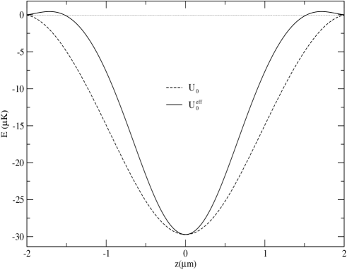
Figure 2: Comparison of lowest-lying Born-Oppenheimer (U₀) and adiabatic (U${}^{eff}_{0}$) curves, for the beamsplitter in Fig. 1

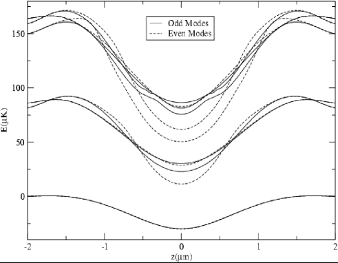
Figure 3: Effective adiabatic potentials for the configuration in Fig. 1. Each curve corresponds to a different transverse mode of the beamsplitter. Because of the intrinsic symmetry of the potential, even and odd modes can be treated separately. The first six even and odd modes of the structure are depicted here.

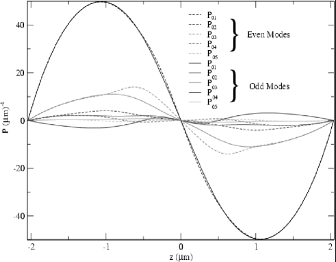
Figure 4: P-matrix elements coupling the first transverse even and odd modes in Fig. 3 to selected higher ones.

Channel coupling is achieved through off-diagonal elements of the $P$ matrix, several of which are shown in Fig.4. As expected, the couplings $P_{0i}$ between the lowest channel 0 and higher channels $i$ diminishes as $i$ gets larger. Also, as implied by Eq.(25) the coupling is strongest where the potential is steepest in the longitudinal direction (i.e. $z=\pm 1$ in the figure).

III.2 General Features of Scattering

Having defined the terms of the problem, and calculated the adiabatic curves and couplings, we solve the scattering equations and extract the S-matrices of the system. All figures shown to this point refer to a beamsplitter with $L=20\mu m$, which is one in which most of the typical features are present. Fig. 5 shows the absolute values of selected S-matrix elements for this configuration, which represent the probabilities for various outcomes. In particular we show the probabilities to exit in the various arm of the beam splitter, assuming unit input flux from the left arm of the splitter, as defined in Fig. 1. At the incident energies shown in Fig. 5, only the lowest mode in each arm is energetically accessible. This typical case is illustrative of the basic elements of the beamsplitter.

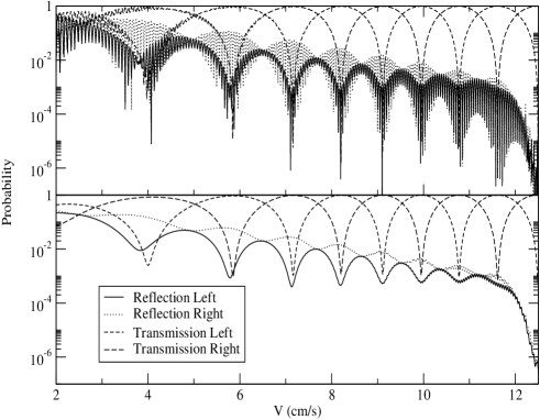
Figure 5: Probability for exit in the various arms of the beamsplitter depicted in Fig. 1, versus incident atom velocity. This figure assumes that the atoms have entered in the lowest mode of the left arm. The velocities shown correspond to atom energies below the second threshold, thus suppressing higher mode excitations. The bottom panel is a $26\mu K$ Gaussian convolution of the one above.

In this beamsplitter the largest probabilities (dashed and short-dashed lines in Fig. 5) correspond to transmission, with the probability alternating between left and right arms. Thus approximately 50-50 beamsplitting is possible at atom energies where these two curves cross. Moreover, the sum of the left and right transmission probabilities is almost, but not quite, equal to unity. This can be seen in the slowly decreasing reflection probabilities (solid and dotted lines) in the figure. The general features of beamsplitting are preserved under a convolution in energy, as exhibited in Fig. 5 b). Here and in what follows, convolution is used to simplify the appearance of the calculations.

The reflection probabilities also exhibit a similar left-right oscillation as a function of energy. In addition, they exhibit a much faster oscillation. This faster oscillation is familiar from one-dimensional scattering from a potential, with one oscillation being added each time the energy increases enough to introduce a new de Broglie wavelength into the scattering region Gas . Here the oscillations are numerous, since the guiding potential is thousands of de Broglie wavelengths long. (These oscillations are of course also present in the transmission probabilities, but are too small to be seen on the scale of the figure.)

For smaller values of $L$ , the beamsplitter is badly non-adiabatic, and even qualitative features of beamsplitting fade. Fig. 6 shows such a non-adiabatic case, with $L=1\mu m$. The effect of the input barrier described in Fig. 2, is now much larger, suppressing all transmission up to input velocities of about 5cm/s. As the kinetic energy reaches the energy of the barrier, the probability exhibits resonant behavior by the presence of spikes in the S-matrices. Though mostly washed out by convolution, these features would in principle cause transparency of the barrier at extremely well defined velocities, where the kinetic energy equals the energy of a metastable boundstate. At higher atom velocities, above the input barrier, reflection remains extremely likely, and even the basic action of the beamsplitter is destroyed.

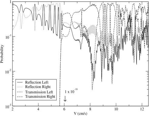
Figure 6: Scattering probabilities as in Fig. 5, but for the extremely non adiabatic case $L=1\mu m$. Only the convolved plot is shown, with a width of 26 $\mu$K.

III.3 Towards Adiabaticity

Fig. 7 shows reflection probabilities versus atom velocity, for various values of the beam-splitter lengths $L$. These results are convolved over an energy width of $16\mu K$, to emphasize the overall probability rather than the oscillatory structure. For $L>2\mu$m, reflection decreases nearly linearly on this semi-log plot, suggesting an exponential decrease of reflection probability with velocity. Reflection also decreases with increasing $L$, as expected for an increasingly adiabatic beamsplitter. The features noticeable around 12.5cm/s and 13.5cm/s represent cusps at the thresholds for the second and third mode to become energetically available, smoothed out by convolution.

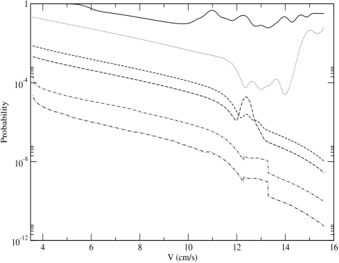
Figure 7: Total reflection probabilities for multi-mode beamsplitter of different lengths. From top to bottom $L=1,2,5,7,15,30\mu m$. The cusps around 12.5 and 13 $cm/s$ are the effects of the second and third thresholds becoming energetically available. The plot represents a $16\mu K$ width Gaussian convolution.

Finally, in Fig. 8 we plot the total transmission to modes higher than the first, for input velocities higher than the second mode threshold. As might be expected, the probability to generate higher modes grows as a function of atom velocity. Countering this trend, the probability again diminishes as the length $L$ becomes longer.

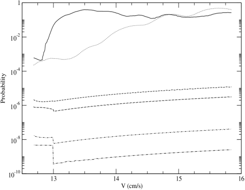
Figure 8: Total transmission to higher modes for different lengths beamsplitter. From top to bottom $L=1,2,5,7,15,30\mu m$. The plot represents a $3.25\mu K$ width Gaussian convolution.

IV Conclusions

We have developed a novel approach to the analysis of non-interacting atomic beams traveling through waveguides, based on the adiabatic representation of scattering theory. This method, originally developed for the study of molecular collision theory, is known to be very flexible, and could be applied to many other guiding geometries. We applied this approach to the study of a two wire atomic beam-splitter, both to illustrate the method and to explore a particular guiding geometry. We have found that the nonadiabatic couplings play a significant role. Because we have deliberately focused on a tightly-confining geometry, it is likely that nonadiabaic effects are even more significant in realistic beamsplitters. This will be a topic of future study.

- (1) W. Hansel, P. Hommelhof, T. W. Hansch, and J. Reichel, Nature 413, 498 (2001).
- (2) A. Kasper et al., J. Opt. B: Quant. Semiclass. Optics, 5: S143 (2003).
- (3) H. Ott, J. Fortágh, G. Schlotterback, A. Grossmann, and C. Zimmerman, Phys. Rev. Lett. 87, 230401 (2001).
- (4) J. Schmiedmayer, Phys. Rev. A 52, R13 (1995).
- (5) J. Denschlag, D. Cassettair, and J. Schmiedmayer, Phys. Rev. Lett. 82, 2014 (1999).
- (6) D. Müller, D. Z. Anderson, R. J. Grow, P. D. D. Schwindt, and E. A. Cornell, Phys Rev. Lett. 83, 5194 (1999).
- (7) N. H. Dekker et al., Phys Rev. Lett. 84, 1124 (2000).
- (8) J. A. Sauer, M. D. Barrett, and M. S. Chapman, Phys. Rev. Lett. 87, 270401 (2001).
- (9) P. Engels, W. Ertmer, and K. Sengstock, Opt. Comm. 204, 185 (2002).
- (10) D. Müller et al., Phys Rev. A 63, 41602 (2001).
- (11) D. Cassettari, B. Hessmo, R. Folman, T. Maier, and J. Schmiedmayer, Phys. Rev. Lett. 85, 5483 (2000).
- (12) D. Müller et al., Optics Letters 25, 1382 (2000).
- (13) A. E. Leanhardt, Y. Shin, A. P. Chikkatur, D. Kielpinski, W. Ketterle, and D. E. Pritchard, Phys. Rev. Lett. 90, 100404 (2003).
- (14) P. D. D. Schwindt, Ph.D thesis, University of Colorado (2003).
- (15) J. A. Stickney and A. A. Zozulya, Preprint.
- (16) M. Jääskeläinen and S. Stenholm, Phys. Rev. A 66, 023608 (2002).
- (17) H. R.Sadeghpour et al., J. Phys B 33 R93 (2000).
- (18) A. A. Zozulya, private communication.
- (19) I. N. Levine, Quantum Chemistry (4th ed., Prentice Hall, Engelwood Cliffs, N. J., 1991).
- (20) M. Jääskeläinen and S. Stenholm, Phys. Rev. A 66, 053605 (2002).
- (21) E. A. Hinds, C. J. Vale, and M. G. Boshier, Phys. Rev. Lett. 86, 1462 (2000).
- (22) J. A. Stickney and A. A. Zozulya, Phys. Rev. A 66, 053601 (2002).
- (23) M. Aymar, C. H. Greene, E. Luc-Koenig, Rev. Mod. Phys. 68, 1015 (1996).
- (24) M. S. Child, Molecular Collision Theory Dover Publications, inc. (1974).
- (25) C. de Boor, A Practical Guide to Splines, Springer (1978).
- (26) H. W. van der Hart, J. Phys. B 30, 453 (1997).
- (27) M. García Sucre, F. Goychman, and R. Lefebvre, Phys. Rev. A 2, 1738 (1970).
- (28) S. Gasiorowicz, Quantum Physics (New York: Wiley, 1974, p. 79).