New combined PIC-MCC approach for fast simulation of a radio frequency discharge at low gas pressure.

Abstract

A new combined PIC-MCC approach is developed for accurate and fast simulation of a radio frequency discharge at low gas pressure and high density of plasma. Test calculations of transition between different modes of electron heating in a ccrf discharge in helium and argon show a good agreement with experimental data. We demonstrate high efficiency of the combined PIC-MCC algorithm, especially for the collisionless regime of electron heating.

I Introduction

The modern trends of plasma technologies are directed to a reduction of the gas pressure and an increase of plasma density. The further development of efficient methods is required for simulation of collisionless regimes in a capacitevely coupled and especially in an inductively coupled discharges as the collisionless heating of electrons plays a key role in dynamics of thin skin layers. The Particle-in-Cell Monte Carlo Collisions (PIC-MCC) method bird has become a standard simulation technique for a gas discharge in plasma reactors of etching or deposition. Unlike the fluid approach, the PIC-MCC algorithm requires larger computer resources, but it provides a detail kinetic picture of processes in a gas discharge. However, a problem of statistical fluctuations of an electric field appears at low gas pressures, in particular for gases with a deep Ramsauer minimum in the elastic scattering cross section. For the periodic electrical field $E=E_{0}\sin(\omega t)$, where $\omega$ is the discharge frequency, the rate of electron heating in the bulk is proportional to $\nu E_{0}^{2}/(\omega^{2}+\nu^{2})$, where $\nu$ is electron collision frequency. At high gas pressure in the collisional regime, when $\nu>\omega$, the electric field in the quasineutral plasma is sufficiently large and the effect the artificial electron heating is less dangerous. At the low gas pressure in the collisionless regime (at $\nu<\omega$), the electrons gain the energy in the electrode sheaths. In the quasineutral plasma the electric field is small and the electrons scattering on the field fluctuations essentially distorts the results. Although the numerical smoothing of the charge density bird2 helps to diminish the statistical noise, it is necessary to develop a more radical way for reduction of the influence of statistical fluctuations.

An interesting idea was suggested in Ref.ivan . As the discharge simulation lasts more than one thousand of discharge periods, the averaging of the charge density over several periods reduces the statistical noise. But the direct averaging can lead to the development of the numerical instability. To eliminate this problem, the electric field was calculated in Ref.ivan from the current continuity equation. However, this approach requires an explicit distinction of electrode sheaths, that is difficult for realization in the two-dimensional case. Besides, it does not take into account inertia of electrons, which is very important at the low gas pressure. Below we present another way of the noise reduction in a new approach developed by Vitaly Schweigert.

II Combined PIC-MCC approach

In the combined PIC-MCC approach we find the electric field distribution from the auxiliary equations which are derived from the kinetic equations. The integration of the electron and ion kinetic equations over the velocity gives us the continuity equations for electron and ion densities. The integration of the kinetic equations multiplied by the velocity gives the continuity equations for electron and ion fluxes. The kinetic coefficients are calculated with using the electron and ion distribution functions, which are found from the electron and ion kinetic equations. To avoid the kinetic coefficients fluctuations we average them over many periods. Thus, in our model the kinetic equations, the auxiliary equations and the Poisson equation are solved self-consistently. The kinetic approach allows us to find the kinetic coefficients and the electric field distribution is found from the auxiliary equation. The equation system includes the Boltzmann kinetic equations for velocity distribution functions of electrons $f_{e}(t,x,\vec{v})$ and ions $f_{i}(t,x,\vec{v})$, which are three dimensional over the velocity and one dimensional in the space

$$\frac{\partial f_{e}}{\partial t}+\vec{v}_{e}\frac{\partial f_{e}}{\partial x}-\frac{e\vec{E}}{m}\frac{\partial f_{e}}{\partial\vec{v}_{e}}=J_{e},\quad n_{e}=\int f_{e}d\vec{v}_{e},$$ (1)

$$\frac{\partial f_{i}}{\partial t}+\vec{v}_{i}\frac{\partial f_{i}}{\partial x}+\frac{e\vec{E}}{M}\frac{\partial f_{i}}{\partial\vec{v}_{i}}=J_{i},\quad n_{i}=\int f_{i}d\vec{v}_{i},$$ (2)

where $v_{e}$, $v_{i}$, $n_{e}$, $n_{i}$, $m$, $M$ are the electron and ion velocities, densities and masses, respectively, $\vec{E}$ is the electrical field, $J_{e}$, $J_{i}$ are the collisional integrals for electrons and ions, the transport equations for the density and the flux of electrons and ions based on the momentum of the kinetic equations (1),(2)

$$\frac{\partial n_{e}^{\prime}}{\partial t}+\frac{\partial j_{e}^{\prime}}{\partial x}=Q,$$ (3)

$$\frac{\partial n_{i}^{\prime}}{\partial t}+\frac{\partial j_{i}^{\prime}}{\partial x}=Q,$$ (4)

$$\frac{\partial j_{e}^{\prime}}{\partial t}=-\frac{\partial T_{e}^{\prime}n_{e}^{\prime}}{\partial x}-\frac{eE}{m}n_{e}^{\prime}-\nu_{e}j_{e}^{\prime}-Q_{e},$$ (5)

$$\frac{\partial j_{i}^{\prime}}{\partial t}=-\frac{\partial T_{i}^{\prime}n_{i}^{\prime}}{\partial x}+\frac{eE}{M}n_{i}^{\prime}-\nu_{i}j_{i}^{\prime}-Q_{i},$$ (6)

where

$$Q=N_{g}\int v\sigma_{i}f_{e}d\vec{v}_{e}$$ (7)

is the ionization rate, $\sigma_{i}$ is the ionization cross sections, $N_{g}$ is the gas density,

$$T_{e}^{\prime}=\frac{\int v_{ex}^{2}f_{e}d\vec{v}_{e}}{\int f_{e}d\vec{v}_{e}},\quad T_{i}^{\prime}=\frac{\int v_{ix}^{2}f_{i}d\vec{v}_{i}}{\int f_{i}d\vec{v}_{i}}$$ (8)

are the effective electron and ion temperatures, respectively,

$$Q_{e}=N_{g}\int v_{ex}|\vec{v}_{e}|\sigma_{t}f_{e}d\vec{v}_{e}-\nu_{e}\int v_{ex}f_{e}d\vec{v}_{e},\quad$$

$$Q_{i}=N_{g}\int v_{ix}|\vec{v}_{i}|\sigma_{r}f_{i}d\vec{v}_{i}-\nu_{i}\int v_{ix}f_{i}d\vec{v}_{i}$$

describe the friction for electrons and ions, the efficient frequencies

$$\nu_{e}=\frac{N_{g}\int|\vec{v}_{e}|\sigma_{t}f_{e}d\vec{v}_{e}}{\int f_{e}d\vec{v}_{e}},\quad\nu_{i}=\frac{N_{g}\int|\vec{v}_{i}|\sigma_{r}f_{i}d\vec{v}_{i}}{\int f_{i}d\vec{v}_{i}},$$ (9)

where $\sigma_{t}$ is the electron transport cross section, $\sigma_{r}$ is the ion resonance charge exchange cross section. Notice that in the usual fluid approach the terms $Q_{e}$, $Q_{i}$ are supposed to be zero, which is correct only for the constant scattering frequencies. The boundary conditions for the auxiliary equations includes the secondary emission as in Ref.Boeuf1987 . It can be easily seen, that the equations (3) -(6) are direct consequences of the kinetic equations (1),(2). As we calculate the kinetic coefficients $Q$, $T_{e}^{\prime}$, $T_{i}^{\prime}$, $Q_{e}$, $Q_{i}$ with solving the kinetic equations (1),(2) with the Monte-Carlo method, the obtained densities $n_{e}^{\prime}$, $n_{i}^{\prime}$ have to coincide with a good accuracy with values from the kinetic equations (1),(2). After calculating the auxiliary values of electron $n_{e}^{\prime}$ and ion $n_{i}^{\prime}$ densities, we calculate the electric field from the Poisson equation

$$\bigtriangleup\phi=4\pi e(n_{e}^{\prime}-n_{i}^{\prime}),\quad E=-\frac{\partial\phi}{\partial x}.$$ (10)

The reduction of statistical noise in our approach is reached with averaging the kinetic coefficients $Q$, $T_{e}^{\prime}$, $T_{i}^{\prime}$, $Q_{e}$, $Q_{i}$ over many periods and with smoothing over the spatial coordinate. For averaging a function $F(x)$ over preceding periods we use the following algorithm

$$F(x)^{i}=\alpha F(x)^{\prime i}+(1-\alpha)F(x)^{i-1},$$ (11)

where $F(x)^{\prime i}$ is the value on the $i$-period and $\alpha=0.01\div 0.1$. The spatial smoothing is chosen as in Ref.bird2

$$F(x_{k})=\frac{F(x_{k+1})+2F(x_{k})+F(x_{k-1})}{4},$$ (12)

where $x_{k}$ is the node of the simulation grid. The spatial smoothing is very important for resolving the space charge in the quasineutral part of a discharge, where the charge is a small difference of two large and almost equal values (ion and electron densities). The computer resources for solving the transport equations (3)-(6) are much smaller than for the kinetic equations, therefore the auxiliary equations are solved for each period, and the kinetic coefficients are calculated after several periods from the kinetic equations (1),(2). Then the electron and ion weights are fitted with the densities $n_{e}^{\prime}$, $n_{i}^{\prime}$. We use $5000$ simulation particles for each charged species, the Cloud-in-Cell charge assignment scheme, the null-collisions technique to find the time of electron and ion free flight, and the energy conserving scheme with a second order of accuracy to solve the equations of motion bird2 ; hock . The equations (3)-(6) are solved with an implicit finite-difference method with using the Scharfetter and Gummel scheme gummel . For small grid spacing $T_{e}\gg e|\phi_{k+1}-\phi_{k}|$ this finite–difference scheme has a second order accuracy in $\bigtriangleup x$ and gives a correct result on rough grids for the Boltzmann electron distribution. Like for the explicit PIC-MCC method, there exists a restriction on time step $\omega_{p}\bigtriangleup t<1$, where $\omega_{p}$ is the plasma frequency, for solution of the equations (3)-(6) with the Poisson equation (10).

Since the cross section of the electron Coulomb scattering is proportional to the electron density and inversely proportional to the square of the electron energy, a correct discharge simulation of some regimes requires accounting for electron Coulomb collisions. For description of these collisions we apply the method manh , where the Langevin force and friction of electrons are introduced and defined from their distribution function. Note also, that the Coulomb collisions do not change the total electron momentum of motion.

The test calculations show that this algorithm is numerically stable and allows one to reach a significant acceleration of the PIC-MCC method due to two factors. At first, the time step for solving the kinetic equations (1),(2) with implicit scheme does not depend on the plasma frequency bird2 ; bird1 . At second, averaging over many periods allows one to reduce greatly (in 5-20 times) the total number of simulation particles in the PIC-MCC method without an increase of the statistical noise.

III How many simulation particles we need?

We study a capacitively coupled radio frequency (ccrf) discharge in argon and helium with the combined PIC-MCC approach for the experimental conditions of Godyak et alGodyak . We consider an one-dimensional symmetrical ccrf discharge at room temperature for the frequency $\nu=13.56~{}MHz$ and with the sinusoidal shape of the discharge current $j$. One electrode is grounded and the voltage on another electrode is calculated self-consistently to provide the desired amplitude of the discharge current. The spatial grid has typically $81$ nodes, condensing in electrode sheaths. The minimal grid spacing is decreased with the gas pressure rise, thus the sheath contains approximately the constant number of nodes. The cross sections of electron scattering in helium are taken from lagu , and for argon from ivan ; lagu . The ion–electron emission on electrodes is taken into account with coefficient $0.2$ in helium and $0.1$ in argon.

It is known that the statistical error of Monte-Carlo methods decreases as $1/N^{2}$. The statistical noise leads to the systematical error in the electron cooling or heating. Therefore, first we have studied the impact of the number of simulation particles on an accuracy of results in three different methods: in the standard PIC-MCC bird , in the PIC-MCC with the spatial smoothing (PIC-MCC SS) bird2 and in our combined PIC-MCC. The simulations are performed for two values of argon pressures $P=0.1,~{}0.3$ Torr, the inter-electrode distance $d=2$ cm and the discharge current $j=2.65$ mA/cm². The mean electron energy in the discharge center calculated with three methods and measured in Ref.Godyak is shown in Fig. 1.

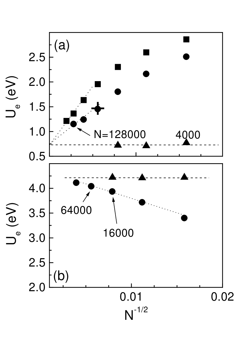
Figure 1: Mean electron energy in the discharge center as a function of the total number of simulation particles for $P=0.1$ Torr (a) and $P=0.3$ Torr (b) calculated with the standard PIC-MCC method (squares), with the PIC-MCC SS method (circles) with spatial smoothing of the space charge and electrical field distributions and with our new combined algorithm (triangles). ’Cross’ is calculation from Ref.bird2 with $N=32000$. $d=2$ cm, $j=2.65$ mA/cm².

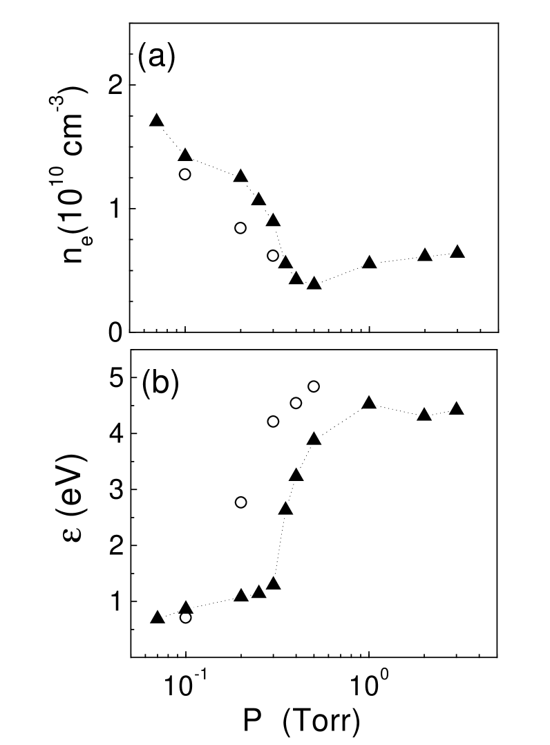
Figure 2: Electron density (a) and mean electron energy (b) in the discharge center ($x=1$ cm) in argon computed (circles) and measured in Godyak (triangles) for $d=2$ cm, $j=2.65$ mA/cm² and $N=5000$.

The calculations with the standard PIC-MCC method with different $N$ show a significant role of electric field fluctuations under the lower gas pressure (squares in Fig. 1(a)). It is seen that the standard PIC-MCC considerably overestimates the value of $\epsilon$ for $N=4000\div 256000$. The second method (PIC-MCC SS) gives much better results (circles in Fig. 1). The spatial smoothing indeed decreases the statistical noise, but feasibility of this technique is restricted, since it distorts the space charge in the electrode sheath. At gas pressure $P=0.3~{}$Torr (see, Fig. 1(b)) when the electron energy $\epsilon$ increases with $N$, the PIC-MCC SS method shows the reasonable accuracy (within $10\%$) with small number of simulation particles $N=10000$. But at the lower pressure $P=0.1$ Torr, the PIC-MCC SS is not able to provide convergency in the electron energy even with $N=256000$. It is obvious that at low gas pressure in order to obtain the reasonable solution with the standard PIC-MCC methods we need so an enormous number of the simulation particles that these methods are not more applicable. As seen in Fig. 1 our combined PIC-MCC method gives the electron energy which is very close to the experimental one (see, Fig. 2) already with the small number of simulation particles and the results only weakly depend on $N$.

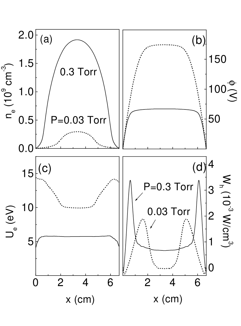
Figure 3: Spatial distribution of averaged over period electron density (a), potential of electric field (b), mean electron energy (c), and electron heating rate (d) in helium for two gas pressures $P=0.03$ (dashed lines) and $0.3$ Torr (solid lines), $d=6.7$ cm, $j=1$ mA/cm² and $N=5000$.

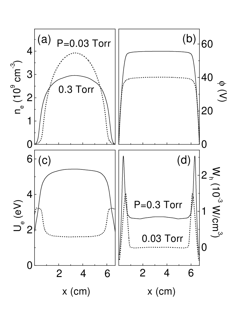
Figure 4: Spatial distribution of averaged over period electron density (a), potential of electric field (b), mean electron energy (c), and electron heating rate (d) in argon for two gas pressures $P=0.03$ (dashed lines) and $0.3$ Torr (solid lines), $d=6.7$ cm, $j=1$ mA/cm² and $N=5000$.

The electron density and the mean electron energy from the experiment Godyak and from the combined PIC MCC simulations with $N=5000$ are shown in Fig. 2 as a function of gas pressure. The calculated dependence of the $\epsilon$ from $P$ demonstrates the transition between different modes of the electron heating found in Godyak and well agrees with the experimental data.

IV Validity of the combined PIC-MCC approach. Simulation results of a ccrf discharge in helium and argon.

Depending on gas pressure, there are two different regimes of electron heating (collision and collisionless) in rf discharges which are well studied experimentally and numerically (see, for example bird ; Godyak ; Levitskii ; Parker ; Vahedi ; Boeuf ). The collision electron heating takes place due to elastic scattering of the electrons on the atoms, when the directed velocity transfers into the thermal one. At high gas pressures the collisonal (or ohmic) heating controls the electron energy in the quasineutral part of the discharge. At the low gas pressure the electrons are heated due to interaction with moving sheaths boundaries and the ohmic heating in bulk is very small. For these two regimes the spatial distributions of the electron density, the electrical potential, the mean electron energy and the electron heating rate $W_{h}=-eE\int v_{ex}f_{e}d\vec{v}_{e}$ are shown in Figs. 3,4 in helium and argon, respectively.

The results are obtained for two different gas pressures $P=0.03$ Torr and $P=0.3$ Torr, for $d=6.7$ cm and $j=1$ mA/cm².

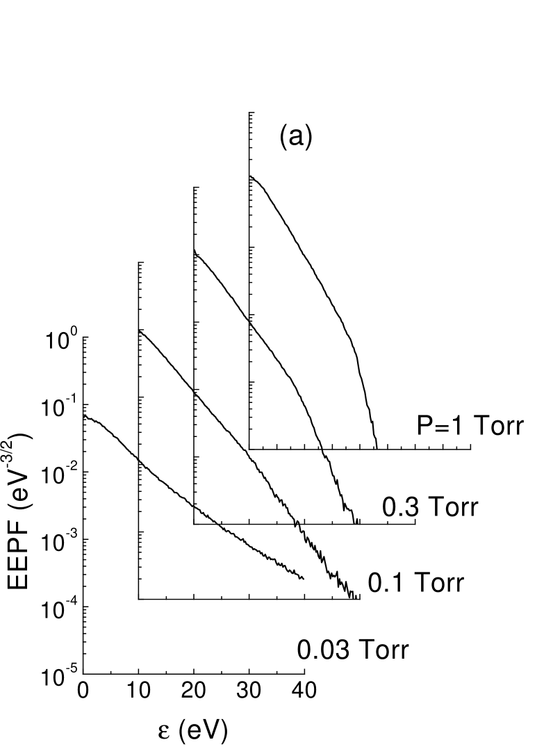
Figure 5: Electron energy probability function in helium in the discharge center ($x=3.35$ cm) for different gas pressures, $d=6.7$ cm, $j=1$ mA/cm² and $N=5000$.

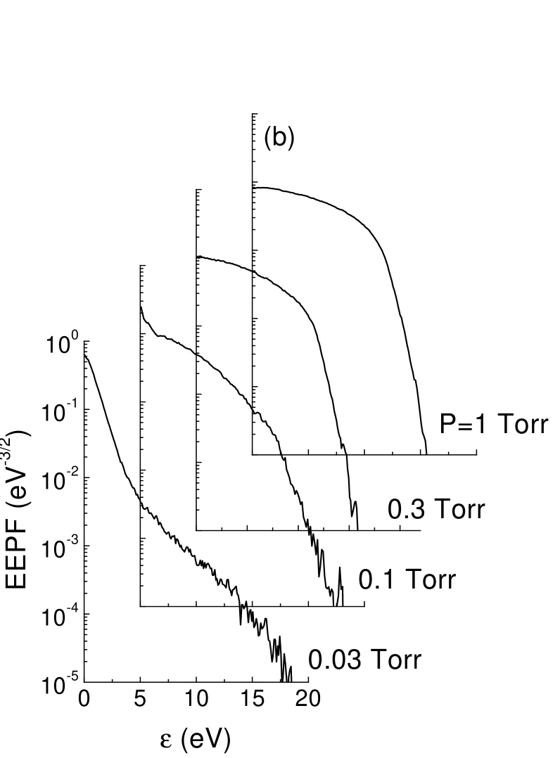
Figure 6: Electron energy probability function in argon in the discharge center ($x=3.35$ cm) for different gas pressures, $d=6.7$ cm, $j=1$ mA/cm² and $N=5000$.

As expected, in helium the mean electron energy increases with pressure lowering in order to compensate an increase of particle losses at the electrodes and in argon we observed the opposite behavior. The reasons of reduction of the electron energy under pressure lowering in argon are discussed in tsendin , where a drop of the electron temperature up to the gas temperature is predicted in the absence of Coulomb electron collisions. Note, that in helium larger heating rate (in the center of discharge) refers to lower $\epsilon$. This non-local effect can not be predicted within the fluid or the diffusion-drift approaches. The electron energy probability functions (EEPF) are shown in Figs. 5,6 for helium and argon. The data presented in these figures averaged over the discharge period. As in the experiment Godyak we also found in argon that the EEPF changes from a Druyvesteyn shape to a bi-Maxwellian one with decreasing the gas pressure (see, Fig. 6). At the low gas pressure the electrons are separated into two groups. The cold electrons are not able to reach the sheath boundary and their ohmic heating is very weak due to Ramsauer minimum in the elastic cross section (see, Fig. 7).

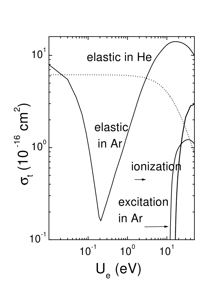
Figure 7: Electron-neutral elastic cross sections in argon (solid line) and in helium (dotted line) as functions of the electron energy.

The fast electrons heated in the sheaths maintain the discharge operation and provide the gas ionization. Fig. 8 presents the computed and measured Godyak electron temperature ($T_{e}=2U_{e}/3$) in the discharge center ($x=3.35~{}cm$).

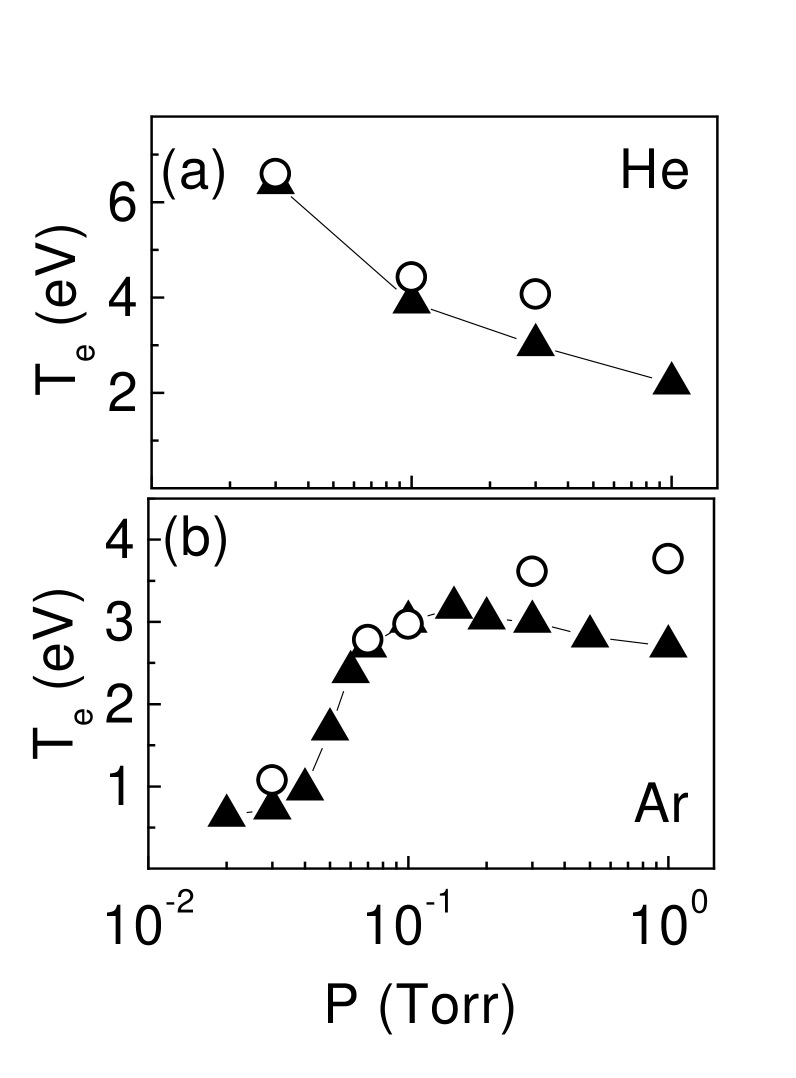
Figure 8: Effective electron temperature ($T_{e}=2U_{e}/3$) in the discharge center ($x=3.35$ cm) in helium (a) and argon (b). Computed $T_{e}$ (circles) and measured $T_{e}$ Godyak (triangles) for $d=6.7$ cm, $j=1$ A/cm² and $N=5000$.

The decrease of the gas pressure is accompanied with a drop of $\epsilon$. A comparison with experimental data shows a good agreement (within $20\div 30\%$) within a pressure range $P=0.03\div 0.3$ Torr for helium and for argon.

The calculation gives higher energy at the larger gas pressure $P=1$ Torr. The difference between computed and measured data at higher gas pressure is likely due to the contribution of metastable states in the ionization kinetics, especially in helium (see, for example Parker ). In the model of electron-neutral collisions in our simulations we do not take into account the multi-step ionization. At low gas pressures we have better agreement because the metastable atoms are deactivated on electrodes and the influence of multi-step ionization reduces. The study of ionization kinetics in noble gases is out of the scope of this article. Note that in our earlier study schweig of the ccrf discharge in helium we have considered the metastable atoms and obtained a good agreement with experimental data for high gas pressures.

In conclusion we have presented the combined PIC-MCC approach for fast simulation of the rf discharge over a wide range of gas pressures and current densities. The validity of the new approach is justified by comparison with the experiment data. The advantage of our approach is the considerable decrease of the number of simulation particles $N$. We are able to reach a speed-up factor of ten for the collision regime and even more for the collisionless regime compared with the standard PIC-MCC calculations.

This work is supported by the NATO Science for Peace Program, Grant No. 974354.

References

- (1) C.K. Birdsall and A.B. Langdon, Plasma Physics Via Computer Simulation, McGraw-Hill, New York (1985).
- (2) C.K. Birdsall, IEEE Trans. Plasma Sci. 10, 65 (1991).
- (3) V.V. Ivanov, A.M. Popov, and T.V. Rakhimova, Plasma Physics 21, 548 (1995)(in Russian).
- (4) J.-P. Boeuf, Phys. Rev. A 36, 2782 (1987).
- (5) R.W. Hockney and J.W. Eastwood, Computer simulation using particles, New York: McGraw-Hill (1981).
- (6) D.L. Scharfetter and H.K. Gummel, IEEE Trans. Electron. Dev. ED31, 1912 (1984).
- (7) W.M. Manheim, M. Lampe, and G. Joyce, J. Comp. Phys. 138, 563 (1997).
- (8) C.K. Birdsall, E. Kawamura, and V. Vahedi Reports of the Institute of Fluid Science 10, 39 (1997).
- (9) V.A. Godyak, R.B. Piejak, and B.M. Alexandrovich, Plasma Sources Sci. Technol. 1, 36 (1992).
- (10) R. Lagushenko and J. Maya, J. Appl. Phys. 59, 3293 (1984).
- (11) S.M. Levitskii, Zh. Tech. Fiz. 27, 1001 (1957) (Sov. Phys. Tech. Phys. 2, 887 (1957)).
- (12) G.J. Parker et al, Physics of Fluids B 5, 646 (1993).
- (13) V. Vahedi et al, Plasma Sources Sci. Technol. 2, 261 (1993).
- (14) Ph. Belenguer and J.-P. Boeuf, Phys. Rev. A 41, 4447 (1990).
- (15) S.V. Bereznoi, I.D. Kaganovich, and L.D. Tsendin, Plasma Physics 24, 603 (1998) (in Russian).
- (16) V.A. Schweigert et al, JETP 88, 482 (1999).