The self-organized multi-lattice Monte Carlo simulation

Abstract

The self-organized Monte Carlo simulations of 2D Ising ferromagnet on the square lattice are performed. The essence of devised simulation method is the artificial dynamics consisting of the single-spin-flip algorithm of Metropolis supplemented by the random walk in the temperature space. The walk is biased to the critical region through the feedback equation utilizing the memory-based filtering recursion instantly estimating the energy cumulants. The simulations establish that the peak of the temperature probability density function is located nearly the pseudocritical temperature pertaining to canonical equilibrium. In order to eliminate the finite-size effects, the self-organized approach is extended to multi-lattice systems, where feedback is constructed from the pairs of the instantaneous running fourth-order cumulants of the magnetization. The replica-based simulations indicate that several properly chosen steady statistical distributions of the self-organized Monte Carlo systems resemble characteristics of the standard self-organized critical systems.

PACS: 05.10.Ln, 05.65.+b, 05.50.+q, 05.70.Jk

1 Introduction

The Monte Carlo (MC) simulation methods are nonperturbative tools of the statistical physics developed hand in hand with increasing power of nowadays computers. The benchmark for testing of MC algorithms represents the exactly solvable Ising spin model [1]. Between algorithms applied to different variants of this model, the using of the single-spin-flip Metropolis algorithm [2, 3] prevails due to its simplicity. Nevertheless the principal problems have emerged as a consequence of the accuracy and efficiency demands especially for the critical region.

As a consequence of this several methods enhancing MC efficiency have been considered. The procedures of great significance are: finite-size-scaling relations and renormalization group based algorithms [4] - [7], cluster algorithms [8, 9] lowering the critical slowing down, histogram and reweighting techniques [10] interpolating the stochastic data, and multicanonical ensemble methods [11] overcoming the tunneling between coexisting phases at 1st order transitions. Even with the mentioned modifications and related MC versions, a laborious and human assisted work is needed until a satisfactory accuracy of results is achieved. This is trivial reason why utilization of the self-organization principles have attracted recent attention of MC community.

In the present paper we deal with the combining of the self-organization principles and MC dynamics. Of course, this effort has a computational rather than physical impact. Our former aim was to design the temperature scan seeking for the position of the critical points of the lattice spin systems. But this original aim has been later affected by the general empirical idea of the self-organized criticality (SOC) [12], originally proposed as a unifying theoretical framework describing a vast class of systems evolving spontaneously to the critical state. The SOC examples are sand pile, forest-fire [13] and game-of-life [14] models. The SOC property can be defined through the scale-invariance of the steady state asymptotics reached by the probability density functions (pdf’s) constructed for spatial and temporal measures of dissipation events called avalanches. The dynamics of standard SOC systems is governed by the specific nonequilibrium critical exponents linked by the scaling relations [15] in analogy to standard phase transitions.

Notice that dynamical rules of standard SOC systems are functions of the microscopic parameters uncoupled to the global control parameters. On the contrary, in the spin systems governed by the single-spin-flip Metropolis dynamics, the spins are flipped according to prescriptions depending on their neighbors, but also on the global or external control parameters, like temperature or selected parameters of the Hamiltonian. The modification, by which the MC spin dynamics should be affected to mimic the SOC properties, is discussed in [16]. In agreement with [17], any such modification needs the support of nonlinear feedback mechanism ensuring the critical steady stochastic state. It is clear that the feedback should be defined in terms of MC instant estimates of the statistical averages admitting the definition of critical state.

The real feedback model called probability-changing cluster algorithm [22] was appeared without any reference to the general SOC paradigm. The alternative model was presented in [18], where temperature of the ferromagnet Ising spin system was driven according to recursive formula corresponding to general statistical theory [19]. This example was based on the mean magnetization leading to series of the temperature moves approaching the magnetic transition. Despite the success in the optimized localization of critical temperature of the Ising ferromagnet, the using of term SOC seems to be not adequate for this case. The reason is the absence of the analysis of spatio-temporal aspects of MC dynamics, which can be considered as a noncanonical equilibrium [20, 21], due to residual autocorrelation of the sequential MC sweeps.

Regarding the above mentioned approaches, the principal question arises, if the MC supplemented by feedback, resembles or really pertains to branch of the standard SOC models which are well-known from the Bak’s original paper [12] and related works.

The plan of our paper is the following. Sec.2 is intended to generalization of the averaging relevant for the implementation of the self-organization principles. The details of feedback construction based on the temperature gradient of specific heat are discussed in Sec.3. These proposals are supplemented by the simulation results carried out for 2D Ising ferromagnet. The details of the multi-lattice self-organized MC simulations, stabilizing true critical temperature via fourth-order magnetization cumulants, are presented in Sec.4. The oversimplified mean-field model of self-organized MC algorithm is discussed in Sec.5. Several universal aspects of the self-organized MC dynamics are outlined by replica simulations in Sec.6. Finally, the conclusions are presented.

2 The running averages

As we already mentioned in introduction, the mechanism by which many body system is attracted to the critical (or pseudocritical) point should be mediated by the feedback depending on the instantaneous estimates of the statistical averages. In this section we introduce the running averages important to construct the proper feedback rules.

Consider the MC simulation generating the sequence of configurations $\{\,X_{t^{\prime}},\,t^{\prime}=1,2,\ldots,\,t\,\}$ according to importance sampling update prescription of Metropolis [3] producing the canonical equilibrium Boltzmann distribution as a function of the constant temperature $T$. The estimate of the canonical average $\langle A\rangle_{t}$ of some quantity $A$

$$\langle A\rangle_{t,T}=\sum_{t^{\prime}=1}^{t^{\prime}=t}w_{t}A_{t^{\prime}}\,\,,\qquad w_{t}=\frac{1}{t}\,.$$ (1)

can simply calculated from the series of $t$ sampled real values $A_{t^{\prime}}\equiv A(X_{t^{\prime}})$ reweighted by $w_{t}$ ensuring the trivial normalization

$$\sum_{t^{\prime}=1}^{t}w_{t}=w_{t}\sum_{t^{\prime}=1}^{t}1=1\,\,\,.$$ (2)

The summation given by Eq.(1) is equivalent to recurrence

$$\langle A\rangle_{t,T}=(1-w_{t})\langle A\rangle_{t-1,T}+w_{t}A_{t}$$ (3)

showing how the average changes due to terminal contribution $A_{t}$. Consider the generalized averaging, where $w_{t}$ is replaced by the constant parameter $0<\eta\ll 1$ which is independent of $t$:

$$\langle A\rangle_{\eta,t,T}=(1-\eta)\langle A\rangle_{\eta,t-1,T}+\eta A_{t}\,.$$ (4)

The consequence of setting $w_{t}\rightarrow\eta$ is the convolution

$$\langle A\rangle_{\eta,t,T}=\sum_{t^{\prime}=-\infty}^{t}w_{\eta,t,t^{\prime}}A_{t^{\prime}}\,\,.$$ (5)

defined by the modified weights

$$w_{\eta,t,t^{\prime}}=\eta\,(1-\eta)^{t-t^{\prime}}\,.$$ (6)

which undergo to normalization

$$\sum_{t^{\prime}=-\infty}^{t}w_{\eta,t,t^{\prime}}=1\,.$$ (7)

For finite initial choice $t^{\prime}=1$ it yields

$$\sum_{t^{\prime}=1}^{t^{\prime}=t}w_{\eta,t,t^{\prime}}=1-(1-\eta)^{t}\,,$$ (8)

where $(1-\eta)^{t}\ll 1$ if the time of averaging is sufficiently large $\eta\ll 1\ll t$. It should be remarked that the generalized averages labeled by $\langle A\rangle_{\eta,t,T}$ are equivalent to gamma filtered [23] fluctuating inputs $A_{t}$. Note that the term gamma originated from the analytic form of the weight $w_{\eta,t,t^{\prime}}$. The filtering represents the application of the selection principle suppressing the information older than the memory depth $\propto 1/\eta$.

3 The specific heat feedback

To attain the critical region self-adaptively we construct the temperature dependent feedback changing the temperature in a way enhancing extremal fluctuations. The running estimates of averages are necessary to predict (with share of the uncertainty) the actual system position and the course in the phase diagram leading to critical point.

The pseudocritical temperature $T_{\rm c}(N)$ of some finite system consisting of $N$ degrees of freedom is defined by the maximum $C(N,T_{\rm c}(N))$ of the specific heat $C(N,T)$. To form an attractor nearly $T_{\rm c}(N)$, we propose the following dynamics of the temperature random walker

$$T_{t+1}=T_{t}+r_{t}\,\Delta\,\,\mbox{sign}(F^{C}_{t})$$ (9)

biased by the gradient

$$F^{C}_{t}=\left.\frac{\partial C}{\partial T}\,\right|_{T=T_{t}}\,,$$ (10)

where $C$ is MC estimate of the specific heat. From that follows that the energy fluctuations are controlled by the temperature representing the additional slowly varying degree of freedom. It is assumed here and in further that $T_{t}$ remains constant during $N$ random microscopic moves ($1$MC step per $N$). The sign function occurring in Eq.(9) is used to suppress the extremal fluctuations of $F^{C}_{t}$ causing the unstable boundless behavior of $T_{t}$. From several preliminary simulations it can be concluded that the replacement of sign function by some smooth differentiable function (e.g. tangent hyperbolic or arcus tangent) seems to be irrelevant for keeping of smaller dispersion of $T_{t}$. The non-constant temperature steps are constrained by $|T_{t+1}-T_{t}|<\Delta$ due to action of the pseudorandom numbers $r_{t}$ drawn from the uniform distribution within the interval $(0,1)$.

Very important for further purposes is the quasi-equilibrium approximation $\langle A\rangle_{t}\simeq\langle A\rangle_{\eta,t,T_{t}}$ justified under the restrictions $t_{{\rm eq},A}\,\eta\ll 1$, $t_{{\rm eq},A}\,\Delta\ll 1$, where $t_{{\rm eq},A}$ is the equilibration time of $A$. With help of this approximation, the running averages from Eq.(4) can be generalized using

$$\langle A\rangle_{\eta,t,T_{t}}=(1-\eta)\langle A\rangle_{\eta,t-1,T_{t-1}}+w_{t}A_{t,T_{t}}\,,$$ (11)

which allow the averaging under the slowly varying temperature. Here $T_{t}$ is the temperature for which the last sample $A_{t,T_{t}}=A(X_{t})$ is calculated.

For later purposes we also introduce the zero passage time $\tau_{A}$ pertaining to $A$. The time is defined as a measure of the stage during which the $\mbox{sign}(A_{t})$ is invariant. More formal definition of $\tau_{A}$ requires the introducing of two auxiliary times $t^{\prime}$, $t^{\prime\prime}$. The first time $t^{\prime}$ defines the instant, where

$$A_{t^{\prime}-1}\,A_{t^{\prime}}\leq 0\,,$$ (12)

whereas $t^{\prime\prime}$ counts the events for which

$$A_{t^{\prime}+t^{\prime\prime}-1}\,A_{t^{\prime}+t^{\prime\prime}}>0\,,\,\,\,\,t^{\prime\prime}=1,2,\ldots\tau_{A}>1\,.$$ (13)

The counting is finished for $t^{\prime\prime}=\tau_{A}$ if

$$A_{t^{\prime}+\tau_{A}}\,A_{t^{\prime}+\tau_{A}+1}\leq 0\,.$$ (14)

To be thorough, the conditions $A_{t^{\prime}-1}\,A_{t^{\prime}}\leq 0$, $A_{t^{\prime}}\,A_{t^{\prime}+1}\leq 0$ should be assumed for definition of $\tau_{A}=1$. Thus, using Eqs.(12)-(14) the original sequence $\{A_{t}\}_{t=1}$ can be transformed to the sequence of passage times $\{\tau_{A}^{(k)}\}_{k=1}$.

From the above definition it follows that random walk in temperature is unidirectional (the sign of $T_{t+1}-T_{t}$ is ensured) for $t^{\prime\prime}=1,2,\ldots,\tau_{F^{C}}$. The arithmetic average of $\tau_{F^{C}}$ is related to temperature dispersion $\langle(\delta T)^{2}\rangle=(\Delta^{2}/3)\langle\tau_{{F^{C}}}\rangle$, where $\langle\tau_{{F^{C}}}\rangle$ is calculated from $\{\tau_{F^{C}}^{(k)}\}_{k=1}$. The standard formula providing $C(T)$ is the fluctuation-dissipation theorem (in $k_{\rm B}$ units)

$$C=\frac{\langle E^{2}\rangle_{t,T}-\langle E\rangle_{t,T}^{2}}{T^{2}N}\,.$$ (15)

Here the specific heat is expressed in terms of the energy $E$ cumulants $\langle E\rangle_{t}$, $\langle E^{2}\rangle_{t}$. In the frame of the quasi-static approximation it is assumed: $T\simeq T_{t}$, $\langle E\rangle_{t,T}\simeq\langle E\rangle_{\eta,t,T_{t}}$, $\langle E^{2}\rangle_{t,T}\simeq\langle E^{2}\rangle_{\eta,t,T_{t}}$. Subsequently, using properties of energy cumulants with equilibrium Boltzmann weights, the temperature derivative of $C$ can be approximated by

$$F^{C}_{t}=\frac{\langle E^{3}\rangle_{\eta,t,T_{t}}-3\langle E\rangle_{\eta,t,T_{t}}\langle E^{2}\rangle_{\eta,t,T_{t}}}{T_{t}^{4}N}$$

$$+2\frac{\langle E\rangle_{\eta,t,T_{t}}^{3}}{T_{t}^{4}N}-2\frac{\langle E^{2}\rangle_{\eta,t,T_{t}}-\langle E\rangle_{\eta,t,T_{t}}^{2}}{T_{t}^{2}N}\,.$$ (16)

Figure 1: The transient regime of $T_{t}$ obtained for several different initial conditions. Simulated for $L=10$, $\eta=10^{-3}$, $\Delta=10^{-4}$ and identical initial values of cumulants.

Figure 2: The pdf distributions obtained for $\eta=10^{-3}$, $\Delta=10^{-4}$, $L=10$: a) the pdf of temperature with the peak located nearly $T_{\rm c}(N)\simeq 0.5868$ (dispersion $0.018$); b) the simulation reveals the flat tails of pdf of $F^{C}_{t}$.

The Ising ferromagnet is simulated in further to study the effect of feedback defined by Eqs.(9), (10) and (16). However, it is worthwhile to note that many of the presented results are of general relevance. Given the spin system $X=\{s_{i}\}_{i=1}^{N}$, $s_{i}=\pm 1/2$ placed at $N=L^{2}$ sites of the square $L\times L$ lattice with the periodic boundary conditions, the Ising Hamiltonian can be defined in exchange coupling units

$$E=-\sum_{\rm nn}s_{i}s_{j}\,,$$ (17)

where nn means that summation running over the spin nearest neighbors.

In general, the dynamics of SOC systems exhibits two distinct regimes. During the transient regime the proximity of critical or pseudocritical point is reached. The second steady regime is called here the noncanonical equilibrium in analogy with [21]. In this regime the attraction to critical point is affected by the critical noise. This general classification is confirmed by our results shown in Figs.1-3. In Fig.1 we see the stochastic paths of $T_{t}$ pertaining to different initial values of energy cumulants and spin configurations. The paths are attracted by $T_{\rm c}(N)$ with some uncertainty in noncanonical equilibrium. For the sufficiently narrow steady pdf’s, $T_{\rm c}(N)$ can be approximated by $T_{\rm c}(N)\simeq N_{\rm av}^{-1}\sum_{t=1}^{N_{\rm av}}T_{t}$, where $N_{\rm av}$ is the number of inputs. The stationary pdf of $T_{t}$ walk is shown in Fig.2a and pdf of $F^{C}_{t}$ with non-Gaussian flat tails is depicted in Fig.2b.

The alternative quantity capable for the characterization of the noncanonical equilibrium is the autocorrelation

$${\cal K}_{\tau}=\frac{1}{N_{\rm av}}\sum_{t=1}^{N_{\rm av}}F^{C}_{t}F^{C}_{t+\tau}\,\,.$$ (18)

The simulations results depicted in Fig.3a evidenced that minimum time for which the anticorrelation ($K_{\tau}<0$) occur is of the order ${\cal O}(\langle\tau_{{F^{C}}}\rangle)$. As we see from Fig.3b, the power-law dependence can be identified within the region of vanishing $\tau_{{F^{C}}}$. More profound discussion of this fact is presented in Sec.6.

Figure 3: The simulation for $L=10$, $\eta=10^{-3}$, $\Delta=10^{-4}$; a) the autocorrelation function $K_{\tau}$; b) the log-log plot of the normalized pdf of zero passage time of $\tau_{{F^{C}}}$ supplemented by the local slope information.

4 Multi-lattice simulations

In this section we try to avoid the problem of finite-size-scaling related to true equilibrium critical temperature $T_{\rm c}$ and critical exponents. The problem is solved by the multi-lattice self-organized simulations based on the dynamical rules treating the information from running averages of magnetization. The considerations are addressed to models, where 2nd order phase transitions take place. The proposal is again applied to 2D Ising ferromagnet on the square lattice.

The quantity indicating deviations of magnetization order parameter $m_{L}=(1/L^{2})\sum_{\langle ij\rangle}s_{i}$ from the gaussianity is the fourth-order cumulant

$$U_{L,T}=1-\frac{\langle m_{L}^{4}\rangle_{t}}{3\langle m_{L}^{2}\rangle_{t}^{2}}\,.$$ (19)

The standard way leading to true $T_{\rm c}=\lim_{N\rightarrow\infty}T_{\rm c}(N)$ is the construction of the temperature dependences $U_{L_{l},T}$, $U_{L_{s},T}$ for two lattices $L_{s}\neq L_{l}$. Then $T_{\rm c}$ follows from the condition of the scale-invariance

$$U_{L_{l},T_{\rm c}}=U_{L_{s},T_{\rm c}}\,\,.$$ (20)

According it the self-organized multi-lattice MC simulation method consists of the following three main points repeated in the canonical order for the counter $t=1,2,\ldots\,$:

1. The performing of $L_{l}^{2}$ spin flips on the lattice indexed by $l$ and $L_{s}^{2}$ spin flips on the second lattice. The flips are generated for fixed temperature $T_{t}$. After it, the instant magnetizations (per site) $m_{L_{l},T_{t}}$ and $m_{L_{s},T_{t}}$ are calculated.

2. The update of the cumulants $\langle m_{L_{l}}^{2}\rangle_{\eta,t,T_{t}}$, $\langle m_{L_{s}}^{2}\rangle_{\eta,t,T_{t}}$, $\langle m_{L_{l}}^{4}\rangle_{\eta,t,T_{t}}$, $\langle m_{L_{s}}^{4}\rangle_{\eta,t,T_{t}}$ according to Eq.(11), which yield to the modified of definition from Eq.(19)

   $$U_{L,T_{t}}=1-\frac{\langle m_{L}^{4}\rangle_{\eta,t,T_{t}}}{3\langle m_{L}^{2}\rangle_{\eta,t,T_{t}}^{2}}\,\,\,.$$ (21)

3. The temperature shift

   $$T_{t+1}=T_{t}+r_{t}\,\Delta\,\mbox{sign}(F_{t,ls}^{U})$$ (22)

   biased to eliminate difference

   $$F_{t,ls}^{U}=U_{L_{l},T_{t}}-U_{L_{s},T_{t}}\,.$$ (23)

   If $L_{l}>L_{s}$ the ordering of cumulants in $F^{U}_{t,ls}$ is chosen subject to assumption

   $$U_{L_{l},T_{t}} > U_{L_{s},T_{t}}\quad\mbox{for}\,\,\,\,\,\,T_{t}<T_{\rm c}\,\,,$$ (24)

   $$U_{L_{l},T_{t}} < U_{L_{s},T_{t}}\quad\mbox{for}\,\,\,\,\,\,T_{t}>T_{\rm c}\,\,.$$

Any modification of the Eqs.(22) and (23) is possible when the preliminary recognition of the critical point neighborhood is performed. The parametric tuning recovers that stabilization of the noncanonical equilibrium via feedback $F_{t,ls}^{U}$ requires smaller $\eta$ and $\Delta$ than single-lattice simulations based on action of $F_{t}^{C}$. The Eq.(22) can be generalized for $n_{\rm r}$ lattices, i.e. for $n_{\rm rp}=\frac{n_{\rm r}}{2}(n_{\rm r}-1)$ competing lattice pairs labeled by $l,s$:

$$T_{t+1}=T_{t}+\frac{r_{t}\,\Delta}{n_{\rm rp}}\,\sum_{l<s=1}^{n_{\rm r}\times n_{\rm r}}\mbox{sign}\left(\,F_{t,ls}^{U}\,\right)\,,$$ (25)

where $1/n_{\rm rp}$ term rescales additive contributions.

The presented method also offers the continuous checking of estimated critical exponents. It comes from the standard assumption that canonical equilibrium magnetization exhibits critical scaling $\langle|m_{L_{j}}|\rangle_{t}=L_{j}^{-\beta/\nu}f_{\rm m}\left(L_{j}(T_{t}-T_{\rm c})\right)$, where $f_{\rm m}(\cdot)$ is the scaling function and $\beta/\nu$ is the ratio of magnetization ($\beta$) and the correlation length ($\nu$) critical exponents, respectively. If the temperature fluctuates nearly $T_{\rm c}$, the equilibrium finite-size-scaling relation changes to $\langle|m_{L_{j}}|\rangle_{\eta,t,T_{t}=T_{\rm c}}\simeq L_{j}^{-\beta/\nu}\,f_{\rm m}(0)$. For $n_{\rm r}\geq 2$ lattices and sufficiently small $\eta$, $\Delta$, the following arithmetic average can be defined

$$\left(\frac{\beta}{\nu}\right)_{\eta,t}=\frac{1}{n_{\rm rp}}\,\sum_{l<s=1}^{n_{\rm r}\times n_{\rm r}}\frac{\ln\left(\frac{\langle|m_{L_{l}}|\rangle_{\eta,t,T_{t}}}{\langle|m_{L_{s}}|\rangle_{\eta,t,T_{t}}}\right)}{\ln\left(\frac{L_{s}}{L_{l}}\right)}\,.$$ (26)

Similar to treatment of the steady temperature fluctuations, the quantity $\beta/\nu\simeq N_{\rm av}^{-1}\sum_{t=1}^{N_{\rm av}}(\beta/\nu)_{\eta,t}$ can be defined. The simulations carried out for cases $n_{\rm r}=2,\,3$ are compared in Fig.4. In agreement with expectation, the localization of $T_{\rm c}$ for $n_{\rm r}=3$ with recursion taken from Eq.(25) is much subtle than for $n_{\rm r}=2$. In addition, the statistics of $(\beta/\nu)_{\eta,t}$ is weakly depending on $\eta$ and $\Delta$, which seems to be logical due to universality of exponents in the canonical equilibrium limit ($T_{\rm c}={\rm const}$).

Figure 4: The stationary statistics of lattices coupled by the fourth-order magnetization cumulants. a) The pdf’s of temperature obtained for parameters $\eta=10^{-3}$, $\Delta=10^{-4}$. $n_{\rm r}=2$ for $L_{1}=10$, $L_{2}=20$ [see (i)]. In that case additional low temperature bound $T_{t}>0.1$ is used to confine dynamics into the region $T_{t}>0$. For $n_{\rm r}=3$, $L_{1}=10$, $L_{2}=16$, $L_{3}=20$ (ii) the stabilization bound is not necessary. For $\eta=10^{-4}$ and for $\Delta=10^{-5}$ the location of $T_{\rm c}$ is much better [ see $n_{\rm r}=2$ (iii) and $n_{\rm r}=3$ (iv)]; b) The comparison of pdf’s of the zero passage time $\tau_{{F^{U}}}$ of two coupled lattice systems of sizes $L_{1}$ and $L_{2}$. Calculated for $\eta=10^{-4}$, $\Delta=10^{-5}$ and $\eta=10^{-4}$, $\Delta=10^{-8}$. The log-log plot of pdf’s results in the slope $-0.671$ in the region of vanishing $\tau_{{F^{U}}}$. For the middle $\tau_{{F^{U}}}$ region the slope is $-0.59$; c) pdf’s of the effective critical index $(\beta/\nu)_{\eta,t}$ obtained for parametric choices from b). The arrow indicates the of exact $T_{\rm c}$.

The $n_{\rm r}=2$ simulations applied for $L_{1}=10$, $L_{2}=20$, $\eta=10^{-4}$, $\Delta=10^{-8}$ leads to the noncanonical equilibrium, for which the temperature average is associated with estimate $T_{\rm c}\simeq 0.5667$ of the exact value $T_{\rm c}^{\rm ex}\simeq[2\ln(1+\sqrt{2}]^{-1}\simeq 0.56729$. The ratio $\beta/\nu\simeq 0.122$ approximates the exact index $(\beta/\nu)^{\rm ex}=0.125$. Much slower walk for $\Delta=10^{-9}$ provides only a insufficient improvement of the previous results. More appealing are estimates $T_{\rm c}=0.5673$, $\beta/\nu\simeq 0.123$ obtained for $n_{\rm r}=3$, $L_{1}=10$, $L_{2}=20$, $L_{3}=30$, $\eta=10^{-4}$, $\Delta=10^{-9}$, $N_{\rm av}=5\times 10^{8}$ with balance of cumulants attained for $U_{L=10,20,30,T_{\rm c}}\simeq 0.61$. Note that $\beta/\nu$ does not change substantially [$\beta/\nu\simeq 0.123(5)$] if estimated from averages $\langle|m_{L_{1}=10}|\rangle_{\eta,t,T_{t}}=0.37$, $\langle|m_{L_{2}=20}|\rangle_{\eta,t,T_{t}}=0.34$, $<|m_{L_{3}=30}|\rangle_{\eta,t,T_{t}}=0.33$.

5 The mean-field analysis of algorithm

In this section we present calculations aimed to understand how the attractivity of critical point arises and how the noncanonical equilibrium is attained by means of feedback. Only a rough approximation of the complex simulation process is considered, where spin degrees of freedom are replaced by the unique magnetization (per site) term $m(t)$. Furthermore, it assumes that the selected central spin $s(t)$ flips in a mean field created by its $z$ neighbors. Let $\pi(t)$ denotes the probability of the occurrence of $s(t)=1/2$ state, then the probability of $s(t)=-1/2$ is $1-\pi(t)$. The master equation for $\pi(t)$ can be written in the form

$$\frac{{\rm d}\pi}{{\rm d}t}=(1-\pi)W^{\mbox{\tiny$[-+]$}}-\pi W^{\mbox{\tiny$[+-]$}}\,.$$ (27)

The Glauber’s [24] heat bath dynamics with the transition probabilities $W^{\mbox{\tiny$[-+]$}}$ and $W^{\mbox{\tiny$[+-]$}}$ between states $s(t)=\pm 1/2$ is preferred in comparison to non-differentiable Metropolis form due to analyticity arguments relevant for formulation by means of differential equation. Within the mean-field approximation it can be assumed

$$W^{\mbox{\tiny$[+-]$}}(t) = \frac{1}{2\tau_{\rm f}}\,\left[1-\tanh\left(\frac{zm(t)}{2T(t)}\right)\right]\,,$$ (28)

$$W^{\mbox{\tiny$[-+]$}}(t) = \frac{1}{2\tau_{\rm f}}\,\left[1+\tanh\left(\frac{zm(t)}{2T(t)}\right)\right]\,.$$

In the above expression $\tau_{\rm f}$ is the time associated with the spin flip process. The expression takes into account $\pm zm(t)$ variations of energy belonging to flips from $s=\pm 1/2$ to $s=\mp 1/2$ given by the effective single-site Hamiltonian $-z\,s(t)\,m(t)$. Assuming that $\pi=m+1/2$ and using Eqs.(27), (28) we obtain

$$\frac{{\rm d}m}{{\rm d}t}=\frac{1}{\tau_{\rm f}}\left[\frac{1}{2}\tanh\left(\frac{zm}{2T}\right)-m\right]$$ (29)

$$\simeq\frac{1}{\tau_{\rm f}}\left[\frac{z-4T}{4T}m-\frac{z^{3}m^{3}}{48T^{3}}+{\cal O}(m^{5})\,\right]\,.$$

Subsequently, the feedback differential equation of the temperature variable is suggested in the form

$$\frac{{\rm d}T}{{\rm d}t}=\alpha\left(\,m^{2}-m_{\rm c}^{2}\,\right)\equiv F^{m}(t)\,,$$ (30)

where $m_{\rm c}$ is the ”nucleation” parameter of the ferromagnetic phase, and $\alpha>0$ is the constant parameter. Unlike the works [18, 19], where feedback consisting of $|m|$ term is considered, the $m^{2}$ is absorbed to the feedback $F^{m}(t)$ proposed here to ensure the analyticity. For $m^{2}>m_{\rm c}^{2}$ the temperature increases, whereas $m^{2}<m_{\rm c}^{2}$ leads to the cooling. The stationary solution of Eqs.(29) and (30) is

$$m_{\rm c}=\frac{1}{2}\tanh\left(\frac{zm_{\rm c}}{2T}\right)\,.$$ (31)

In the limit of vanishing $m_{\rm c}$, the solution of Eq.(31) can be written in terms of the inverse Taylor series in $m_{\rm c}$

$$T=\frac{z}{4}\left(1-\frac{4m_{\rm c}^{2}}{3}\right)+{\cal O}(m_{\rm c}^{4})\simeq T_{\rm c}^{\rm MF}\,,$$ (32)

where $m_{\rm c}=0$ corresponds to the known mean-field critical temperature $T_{\rm c}^{\rm MF}=z/4$. Small negative shift of stationary $T$ from Eq.(32) caused by $m_{\rm c}\simeq 0$ corresponds to Fig.5 including the numerical solution of Eqs.(29) and (30).

Figure 5: The numerical solution of differential equations Eqs.(29) and (30) is presented. The transient dynamics of the temperature obtained for $m_{\rm c}=0.005$, $\alpha=10^{-3}$ and initial conditions $T|_{t=0}=0.125$, $m|_{t=0}=0.05$ .

6 The comparison of MC and SOC dynamics.

In the section we discuss the universal aspects of the non-equilibrium self-organized MC dynamics applied to the canonical Ising model. As is already mentioned, the attributes of the SOC systems are avalanches reflected by the power-law pdf distributions. We follow with the construction of certain temporal characteristics by supposing their uncertain links to avalanches. By using Eqs.(12)-(14) the evolution of any quantity can be mapped to the sequence of passage times. The example of this view represents pdf of $\tau_{F^{C}}$ depicted in Fig.2. Because of the substantial difference in the exponents of pdf’s belonging to $\tau_{F^{C}}$ and $\tau_{F^{U}}$, no universality attributes are indicated. More encouraging should be to find of pdf’s independent of the feedback type. The natural way toward this aim seems to be the investigation of the passage time sequences linked to the order parameter of the canonical equilibrium of given system. In the case of the Ising model the ordering is described by the magnetization, or, eventually by isolated spin value. Therefore, it seems to be logical to define the passage times $\tau_{m}$, $\tau_{s}$ given by Eqs.(12)-(14) (corresponding to $A=m_{L},s_{i}$, where $i$ is the arbitrary but fixed site position). The simulation results are depicted in Fig.6.

Figure 6: The comparison of stationary pdf’s of zero passage times $\tau_{s}$ and $\tau_{m}$ of different lattice sizes and different feedbacks. Simulated for $\eta=10^{-4}$ and $\Delta=10^{-5}$. The figure shows rescaled pdf’s of different systems subject to settings ordered to three-component tuples: [feedback type, (quantity leading to $\{\tau_{A}^{(k)}\}$ sequence), system size]: (i), $F^{C}_{t}$, ($A=m_{L}$), $L=10$; (ii), $F^{U}_{t}$, ($A=s_{i}$), $L=10$; (iii), $F^{U}_{t}$, ($A=m_{L}$), $L=10$; (iv), $F^{U}_{t}$, ($A=s_{i}$), $L=10$; (v), $F^{C}_{t}$, ($A=s_{i}$), $L=200$; (vi), $F^{C}_{t}$, ($A=s_{i}$), $L=50$; (vii), $F^{C}_{t}$, ($A=s_{i}$), $L=4$;

In their structure, the following attributes relevant for interpretation in terms of SOC can be identified:

• the power-law behavior

  $${\rm pdf}(\tau_{s})\simeq\tau_{s}^{-\phi}\,,\qquad\phi\simeq 1.3$$ (33)

  with the unique exponent $\phi$ pertaining to different feedbacks $F_{t}^{C}$, $F_{t}^{U}$, i.e. to single- lattice and two-lattice systems;

• the interval of dependence from (I) broaden with the size of lattices

• the exponent $\phi$ (at the present level of accuracy) indistinguishable for pdf’s taken for sequences $\{\tau_{s}^{(k)}\}_{k=1}$ and $\{\tau_{m}^{(k)}\}_{k=1}$.

The high-temperature limit of pdf of $\{\tau_{s}^{(k)}\}_{k=1}$ can be easily derived due to assumption about the absence of spin-spin correlations. Its form

$${\cal P}_{\tau_{s}}(p)=(1-p)^{L^{2}\tau_{s}-1}p\,,\qquad p=1/L^{2}\,$$ (34)

expresses invariance of $s_{i}$ during $(\tau_{s}-1/L^{2})$ spin flips, and its immediate change after the $\tau$th spin flip occurring with probability $p$ of the random picking of $i$th site. The simulations carried for paramagnet $T\gg T_{\rm c}$ depicted in Fig.7 agree with formula Eq.(34).

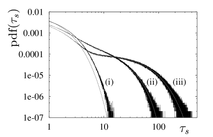
Figure 7: The pdf of the spin passage times obtained for $L=10$, $\eta=10^{-4}$, $\Delta=10^{-6}$. The MC simulations for fixed temperatures (i) $T=4\,T_{\rm c}(N)$ (para-phase); black-dashed line corresponding to ${\cal P}_{\tau_{s}}$ from Eq.(34); (iii) $T=0.8\,T_{\rm c}(N)$ (ferro-phase). The white-dashed line is the fit of the ”bimodal” pdf ${\cal P}_{\tau_{s}}$. Compared with self-organized MC simulations (ii), where feedback $F_{t}^{C}$ yields to the power-law behavior with exponent from Eq.(33).

Below $T_{\rm c}$ pdf splits into separable contributions fitted here by the bimodal distribution $P_{\tau_{s}}=b_{0}{\cal P}_{\tau_{s}}(p_{0})+b_{1}{\cal P}_{\tau_{s}}(p_{1})$ with parameters $b_{0}=0.003$, $b_{1}=0.004$, $p_{0}=0.61$, $p_{1}=0.02$. The supplementary analysis of statistics of the successive time differences of $m_{L}$ recovers that $b_{1}{\cal P}_{\tau_{s}}(p_{1})$ term originates from the mechanism of the long-time tunneling among nearly saturated states of the opposite polarity. From the figure it also follows that power-law short-time regime described by Eq.(33) is formed only if the feedback mechanism is activated. This conditional occurrence of universality can be considered as an additional (IV)th attribute relevant for identification of SOC. The noncanonical equilibrium attained by the self-organized MC dynamics for $L=10$ leads to $P_{\tau_{s}}$ dependence, which can be approximated by the fit

$$P_{\tau_{s}}=b_{2}\,\tau_{s}^{-\phi}\exp\left[-\left(\frac{\tau_{s}}{\tau_{2}}\right)^{2}\right]$$ (35)

with parameters $b_{2}=0.00264$, $\tau_{2}=43.521$.

Let us to note that for the sand pile model [12] the spatial measure of avalanche is associated with the energy integral taken during the stage following disturbance. In the case of MC the analog of spatial measure can be the extremal magnetization

$$m_{\rm max}^{(k)}=\begin{array}[]{c}\mbox{max}\\ \mbox{ \tiny$t=t^{(k)}_{m}+1,\ldots,t^{(k+1)}_{m}$ }\end{array}{\Big{|}}m_{L_{s},T_{t}}{\Big{|}}\,,$$ (36)

where $t_{m}^{(k)}=\sum_{j=1}^{k}\tau_{m}^{(j)}$. The simulations show that pdf corresponding to sequence $\{m_{\rm max}^{(k)}\}_{k=1}$ can be approximated by ${\rm pdf}(m_{\rm max})\propto(m_{\rm max})^{-\phi_{m}}$ with $\phi_{m}=-2.0\pm 0.1$ obtained for the narrow span $m_{\rm max}\in<0.2,\,0.4>$. In agreement with SOC attribute labeled I, the independence of feedback type is identified.

It should be noticed that there remains the principal problem of the link between SOC and presented self-organized MC method focused to the critical region. The problem is to identify the specific algorithmic segment which should be interpreted as an analogue of a disturbance initializing the avalanche. Fortunately, the advanced MC approach exists through which a disturbance can be absorbed into MC algorithm with minor violation of the original dynamics. In general, the approach of interest based on the coevolution of given system and its replica is known under the term damage spreading technique [25]. To apply it, let us consider the self-organized MC referential system labeled here as $\{1\}_{t}$, which incorporates instant cumulants (single with $F^{C}_{t}$ or multi-lattice based on $F^{U}_{t}$), spin configurations and instant temperature $T_{t}^{\{1\}}$. Consider also the replica counterpart $\{2\}_{t}$ of the system $\{1\}_{t}$. As is known, the parallel simulation of $\{1\}_{t}$ and $\{2\}_{t}$ should be applied with the identical pseudorandom sequences. Canonically, the measure of damage effect is then defined through the single-time two-replica difference

$$D^{\{1,2\}}_{t}=m^{\{1\}}_{L_{l},T_{t}^{\{1\}}}-m^{\{2\}}_{L_{l},T_{t}^{\{2\}}}\,,$$ (37)

where $m^{\{1\}}_{L_{l},T_{t}^{\{1\}}}$ and $m^{\{2\}}_{L_{l},T_{t}^{\{2\}}}$ are magnetizations of two lattices of the same size $L_{l}$ belonging to systems $\{1\}_{t}$ and $\{2\}_{t}$. Using Eqs.(12)-(14) the sequence of differences $A_{t}\equiv D^{\{1,2\}}_{t}$, $t=1,2,\ldots$ is mapped onto the sequence of passage times $\tau_{D}^{(k)}$, $k=1,2,\ldots$. In the case when $t$ coincides with one time between $t_{D}^{(k)}=\sum_{j=1}^{k}\tau_{D}^{(j)}$, the replica $\{2\}_{t_{D}^{(k)}}$ is rebuilded within two steps:

1. all of the instant cumulants and spin configurations involved in ${\{2\}}_{t}$ are replaced by ${\{1\}}_{t}$, i.e. $D^{\{1,2\}}_{t_{D}^{(k)}}=0$.

2. the replica temperature is modified according

   $$T_{t=t_{D}^{(k)}}^{\{2\}}=T_{t=t_{D}^{(k)}}^{\{1\}}+\epsilon_{T}\,,$$ (38)

   where constant $\epsilon_{T}$ causes the small disturbance of the coincidence of the contents of $\{1\}_{t_{D}^{(k)}}$ and $\{2\}_{t_{D}^{(k)}}$.

Evidently, the temperature disturbance plays role similar to adding of the grain to the sand pile. The sand pile is stabilized if the rest state occurring for $t=t_{D}^{(k)}+\tau_{D}^{(k)}$ is reached. The main idea of replica approach is that the relative motion of $\{2\}_{t}$ with respect to $\{1\}_{t}$ enhances the nonlinearity responsible for a wide range of $D_{t}^{\{1,2\}}$ responses to $\epsilon_{T}$. Thus, the only stochastic elements of replica simulation originate from the instants over which the content of $\{2\}_{t=t_{D}^{(k)}}$ is replaced by the content of $\{1\}_{t=t_{D}^{(k)}}$. In analogy to Eq.(36), the complementary measure reflecting the spatial activity can be

$$D_{\rm max}^{(k)}=\begin{array}[]{c}\mbox{max}\\ \mbox{\tiny$t=t^{(k)}_{\rm D}+1,\ldots,t^{(k+1)}_{D}$ }\end{array}{\Big{|}}D_{t}^{\{1,2\}}{\Big{|}}\,.$$ (39)

Using this, the simulated path is mapped onto the sequence $\{D_{\rm max}^{(k)}\}_{k=1}$. Consequently, the pdf’s can be extracted which are depicted in Fig.8. They show that the effective exponents centred nearly $-2.3$ fit simulated pdf’s fairly well. As in the case labeled I, pdf’s related to $\tau_{D}^{(k)}$ and $D_{\rm max}^{(k)}$ are weakly susceptible to the feedback choice. Since both temporal and spatial power-law attributes of universality are indicated, the standard SOC paradigm can be considered as a framework adaptable for the analysis of the suggested self-organized MC dynamics.

Figure 8: The stationary power-law pdf distributions of the passage times $\tau_{D}$ calculated for different feedbacks (SOC criterion no.I) $F^{C}_{t}$, $F^{U}_{t}$, self-organization parameters $\eta=10^{-4}$, $\Delta=10^{-5}$ and disturbance parameter $\epsilon_{T}=10^{-3}$ for sizes $L_{1}=10$, $L_{2}=20$.

7 Conclusions

Several versions of MC algorithm combining the self-organization principles with the MC simulations have been designed. The substantial feature of method is the establishing of running averages coinciding with gamma filtering of the noisy MC signal. The simulations are combined with the mean-field analysis describing the motion of temperature near to magnetic transition point. The replica-based simulations indicate that pdf distributions of passage times in a noncanonical equilibrium attain the interval of the power-law behavior typical for the standard SOC pdf distributions. We hope that the present contribution will stimulate further self-organized studies of diverse lattice models, e.g. those related to percolation problem.

Acknowledgement

The authors would like to express their thanks to Slovak Grant agency VEGA (grant no.1/9034/02) and internal grant VVGS 2003, Dept.of Physics, Šafárik University, Košice for financial support.

References

- [1] L. Onsager, Phys. Rev. 65, 117 (1944); R.J. Baxter, Exactly Solved Models in Statistical Mechanics, Academic Press, London, 1982
- [2] K. Binder, D.W. Heermann, Monte Carlo Simulation in Statistical Physics, Springer, Berlin 1998
- [3] N. Metropolis, A.W. Rosenbluth, M.N. Rosenbluth and A.H. Teller, J.Chem.Phys. 21, 1087 (1953).
- [4] S. Ma, Phys. Rev. Lett. 37, 461 (1976).
- [5] R.H. Swendsen, Phys.Rev.B 20, 2080 (1979).
- [6] K.E. Schmidt, Phys.Rev.Lett. 51, 2175 (1983).
- [7] H.H. Hahn and T.S.J. Streit, Physica A 154, 108 (1988).
- [8] R.H. Swendsen and J.S. Wang, Phys.Rev.Lett. 58, 86 (1987).
- [9] U. Wolff, Phys.Rev.Lett. 62, 361 (1989).
- [10] A.M. Ferrenberg and R.H. Swendsen, Phys.Rev.Lett. 61, 2635 (1988); A.M. Ferrenberg and R.H. Swendsen, Phys.Rev.Lett. 63, 1195 (1989).
- [11] B.A. Berg and T.Nehaus, Phys.Rev.Lett 68, 9 (1992).
- [12] P. Bak, C. Tang and K. Wiesenfeld, Phys.Rev.A 38, 364 (1988); P. Bak, C. Tang and K. Wiesenfeld, Phys.Rev.Lett. 59, 381 (1987).
- [13] B. Drossel and F. Schwabl, Phys.Rev.Lett. 69, 1629 (1992).
- [14] P. Alstrom, J. Leo, Phys.Rev.Lett. 49, R2507 (1994).
- [15] C. Tang and P. Bak, Phys.Rev.Lett. 60, 2347 (1988).
- [16] D. Sornette, A. Johansen and I. Dornic, J. Phys. I France 5, 325 (1995).
- [17] L.P. Kadanoff, Physics Today (March 1991) p. 9
- [18] U.L. Fulco, L.S. Lucerna and G.M. Viswanathan, Physica A 264, 171 (1999).
- [19] H. Robbins and S. Munroe, Ann. Math. Stat. 22, 400 (1951).
- [20] J.R.S. Leo, B.C.S. Grandi and W. Figueiredo, Phys.Rev.E 60, 5367 (1999).
- [21] P. Buonsante, R. Burioni, D. Cassi and A. Vezzani, Phys.Rev.E 66, 36121 (2002).
- [22] Y. Tomita and Y. Okabe, Phys. Rev. Lett. 86, 572 (2001).
- [23] J.C. Principe, N.R. Euliano and W.C. Lefebvre, Neural and adaptive systems: Fundamentals through simulations. 2000 John Wiley & Sons, Inc.
- [24] R.J. Glauber, J. Math. Phys. 4, 294 (1963).
- [25] B. Zheng, Int. J. Mod. Phys. B 12, 1419 (1998).