Scattering matrix approach to the resonant states and $Q$-values of microdisk lasing cavities.

Abstract

We have developed a scattering-matrix approach for numerical calculation of resonant states and $Q$-values of a nonideal optical disk cavity of an arbitrary shape and of an arbitrary varying refraction index. The developed method has been applied to study the effect of surface roughness and inhomogeneity of the refraction index on $Q$-values of microdisk cavities for lasing applications. We demonstrate that even small surface roughness ($\Delta r\lesssim\lambda/50$) can lead to a drastic degradation of high-$Q$ cavity modes by many orders of magnitude. The results of numerical simulation are analyzed and explained in terms of wave reflection at a curved dielectric interface combined with the examination of Poincaré surfaces of section and Husimi distributions.

I Introduction

Dielectric and polymeric microcavities represent a great potential for possible applications in lasing optoelecronic devices Yamamoto ; Nockel . In conventional lasers, a significant fraction of optical pump power is lost and a rather high threshold power is needed to initiate the lasing effect. In contrast, spherical and disk cavities can be used to support highly efficient low-threshold lasing operation. The high efficiency of such devices is related to the existence the natural cavity resonances. These resonances are known as morphology-dependent resonances or whispering gallery modes Hill_Benner . The nature of these resonances can be envisioned in a ray optic picture, when light is trapped inside the cavity through the total internal reflection on the cavity-air boundary.

In dielectric cavities optically pumped quantum wells, wires or dots provide an active medium sustaining the lasing operation Slusher_1992 ; Slusher_1993 ; Fujita ; Gayral ; Seassal . Polymeric microcavity lasers are made with an active medium including host and guest molecules Berggren ; Inganas ; Polson2002 . The absorbed light is transferred from the photoexcited host molecules in the non-radiative way by means of resonant energy transfer to the guest molecules. A stimulated emission from the active medium of dielectric and polymeric cavities is trapped in high-$Q$ modes for a very long time. This leads to a significant increase of intensity of radiation inside the cavity and hence to low-threshold laser operation.

One of the most important characteristics of cavity resonances is their quality factor ($Q$-factor) defined as $Q=2\pi*$(Stored energy)/(Energy lost per cycle). The high value of the $Q-$factor results from very low radiative losses that are mainly caused by radiation leakage due to diffraction on the curved interface. An estimation of the $Q$-factor in an ideal circular disk cavity of a typical diameter $d\sim 10\mu$m for a typical WG resonance gives $Q\sim 10^{13}$ (see below, Eq. (46)). At the same time, experimental measured values reported so far are typically in the range of $10^{3}\sim 10^{4}$ or lower Slusher_1992 ; Slusher_1993 ; Fujita ; Gayral ; Seassal ; Berggren ; Inganas ; Polson2002 . A reduction of a $Q$-factor may be attributed to a variety of reasons including side wall geometrical imperfections, inhomogeneity of the diffraction index of the disk, effects of coupling to the substrate or pedestal and others. A detailed study of the effects of the above factors on the characteristics and performance of the microcavity lasers appears to be of crucial importance for the design, tailoring and optimization of $Q$-values of lasing microdisk cavities. Such the studies would require an effective computational method that can deal with both complex geometry and variable refraction index in the cavity.

One of the most powerful and versatile numerical techniques often used in photonic simulation is the finite difference time domain method (FDTD) Yee ; Li ; Sadiku . A severe disadvantage of this technique in application to the cavities with small surface imperfections is that the smooth geometry of the cavity has to be mapped into a discrete grid with very small lattice constant. This makes the application of this method to the problem at hand rather impractical in terms of both computational power and memory.

Another class of computational methods reduces the Helmholtz equation in the infinite two-dimensional space into contour integral equations defined at the cavity boundaries. These methods include the $T$-matrix technique Waterman ; Mishchenko , the boundary integral methods Knipp ; Wiersig , and others Boriskina . These methods are computationally effective and capable to deal with the cavities of arbitrary geometry. However, the above methods require the refraction index be constant inside the cavity boundary.

In the present paper we develop a new, computationally effective, and numerically stable approach based on the scattering matrix technique that is capable to deal with both arbitrary complex geometry and inhomogeneous refraction index inside the cavity. Note that the scattering matrix technique is widely used in analysis of waveguidesRussian as well as in quantum mechanical simulationsDatta . This technique was also used for the analysis of resonant cavities for geometries when the analytical solution was availableHentschel .

The main idea of the method consists of dividing the cavity region into $N$ narrow concentric rings. At each $i$-th boundary between the neighboring rings we calculate the scattering matrix $\mathbf{S^{i}}$ that relates the states propagating (or decaying) towards the boundary, with those propagating (or decaying) away of the boundary. Successively combining the scattering matrixes for all the boundariesRussian ; Datta , $\mathbf{S^{1}}\otimes\ldots\otimes\mathbf{S^{N}}$, we eventually relate the combined matrix to the total scattering matrix of the cavity $\mathbf{S}$. In order to calculate the lifetime of the cavity modes (and, therefore their $Q$-factor) we compute the Wigner-Smith lifetime matrixSmith which, in turn, is expressed in terms of the total scattering matrix $\mathbf{S}$ Smith ; Mello ; Nockel .

Because at each step we combine only two scattering matrixes, it is not required to keep track of the solution in the whole space. This obviously eliminates the need for storing large matrices and facilitates the computational speed. It is also well known that the scattering matrix technique (in contrast, for example, to the transfer matrix technique) is not plagued by numerical instability, because exponentially growing and decaying evanescent waves are separated in course of the computation. Note that the present technique of combining $S$-matrixes is conceptually similar to the recurrence algorithm for calculating electromagnetic scattering from a multilayered sphere Wu ; Johnson . However, in contrast to these works, the scattering matrix technique presented here can be applied to the systems where the refraction index varies as a function of both radial and angular coordinates.

The paper is organized as follows. In Section II.1 we develop the scattering matrix technique for disk-shaped cavities. The results of numerical calculations of resonant states and $Q$-values of nonideal cavities on the basis of the developed technique are presented in Section III. We consider and compare two cases, a disk cavity of a constant refraction index $n$ with side wall imperfection (surface roughness), and, a disk cavity of an ideal circular shape but with inhomogeneous refraction index $n=n(r,\varphi)$. The results of numerical simulation are analyzed and explained in terms of wave reflection at a curved dielectric interface combined with the examination of Poincaré surfaces of section and Husimi function. Finally, we present our conclusion in Section IV.

II The scattering matrix approach

II.1 Formalism

We consider a two-dimensional cavity with the refraction index $n$ surrounded by air. Because the majority of experiments are performed only with the lowest transverse mode occupied, we neglect the transverse ($z$-) dependence of the field and thus limit ourself to the two-dimensional Helmholtz equation. The two-dimensional Helmholtz equation for $z$-components of electromagnetic field is given by

$$\left(\frac{\partial^{2}}{\partial{r^{2}}}+\frac{1}{r}\frac{\partial}{\partial{r}}+\frac{1}{r^{2}}\frac{\partial^{2}}{\partial{\varphi^{2}}}\right)\Psi(r,\varphi)+(kn)^{2}\Psi(r,\varphi)=0,$$ (1)

where $\Psi=E_{z}\ (H_{z})$ for TM (TE)-modes, and $k$ is the wave vector in vacuum. Remaining components of the electromagnetic field can be derived from $E_{z}\ (H_{z})$ in a standard way.

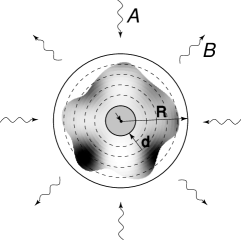
Figure 1: Schematic geometry of a cavity with the refraction index $n$ surrounded by air. The space is divided in three regions. In the inner ($r<d$) and in the outer regions ($r>R$) the refraction indexes are constant. In the intermediate region $d<r<R$ the refraction index $n$ is a function of both $r$ and $\varphi$. The intermediate region is divided by $N$ narrow concentric rings. In each ring the refraction coefficient is regarded as a function of the angle only, $n_{i}=n_{i}(\varphi)$.

We divide our system in three region, the outer region, $r>R$, the inner region, $r<d$, and the intermediate region, $d<r<R$, see Fig. 1. We choose $R$ and $d$ in such a way that in the outer and the inner region the refraction indexes are independent of the coordinate, whereas in the intermediate region $n$ is a function of both $r$ and $\varphi$. In the outer region the solution to the Helmholtz equation can be written in the form

$$\Psi_{out}=\sum_{q=-\infty}^{+\infty}\left(A_{q}H_{q}^{(2)}(kr)+B_{q}H_{q}^{(1)}(kr)\right)e^{iq\varphi},$$ (2)

where $H_{q}^{(1)},H_{q}^{(2)}$ are the Hankel functions of the first and second kind of the order $q$ describing respectively incoming and outgoing waves.

We define the scattering matrix $\mathbf{S}$ in a standard fashion Datta ; Russian ,

$$B=\mathbf{S}A,$$ (3)

where $A,B$ are the column vectors composed of the expansion coefficients $A_{q},B_{q}$ in Eq. (2). The matrix element $S_{q^{\prime}q}=(\mathbf{S})_{q^{\prime}q}$ gives a probability amplitude of the scattering from the incoming state $q$ into the outgoing state $q^{\prime}$. Because of the requirement of the flux conservation, the scattering matrix is unitary Datta ,

$$\mathbf{S}\mathbf{S}^{\dagger}=\mathbf{I},$$ (4)

where $\mathbf{I}$ is the identity matrix. The time reversal invariance imposes the symmetry requirement upon the scattering matrix Datta ,

$$S_{q^{\prime}q}=S_{qq^{\prime}}.$$ (5)

These two conditions can be used to control numerical results for the scattering matrix.

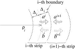
Figure 2: The intermediate region is divided by $N$ concentric rings of the width $2\Delta$; $\rho_{i}$ is the distance to the middle of the $i$-th ring. States $a^{i},a^{i+1}$ propagate (or decay) towards the $i$-th boundary, whereas states $b^{i},b^{i+1}$ propagate (or decay) away of this boundary. The $i$-th boundary is defined as the boundary between the $i$-th and ($i+1$)-th rings.

In order to apply the scattering matrix technique we divide the intermediate region into $N$ narrow concentric rings, see Figs. 1, 2. Within each $i$-th ring we write down the solution to the Helmholtz equation as a linear superposition of the states propagating (or decaying) out of the disk center and the states propagating (or decaying) towards the disk center (the detailed form of these states will be given in Section II.2, see Eq. (40)). At each $i$-th boundary (defined as a boundary between the $i$-th and $i+1$-th rings) we can introduce the scattering matrix $\mathbf{S^{i}}$ that relates the states propagating (or decaying) towards the boundary, $\{a^{i}_{m}\}$ and $\{a^{i+1}_{m}\}$, with those propagating (or decaying) away of the boundary, $\{b^{i}_{m}\}$ and $\{b^{i+1}_{m}\}$,

$$\left(\begin{array}[]{ll}b^{i}\\ b^{i+1}\end{array}\right)=\mathbf{S^{i}}\left(\begin{array}[]{ll}a^{i}\\ a^{i+1}\end{array}\right),\quad 1\leq i\leq N-1,$$ (10)

where $a^{i},b^{i}$ are the column vectors composed of the expansion coefficients $\{a^{i}_{m}\},\{b^{i}_{m}\}$, see below, Eq.(40). For the $N$-th boundary between the last $N$-th ring and the outer region the scattering matrix $\mathbf{S^{N}}$ is defined in the form

$$\left(\begin{array}[]{ll}b^{N}\\ B\end{array}\right)=\mathbf{S^{N}}\left(\begin{array}[]{ll}a^{N}\\ A\end{array}\right).$$ (15)

In the inner region ($i=0$) the solution to the Helmholtz equation has the form

$$\Psi_{in}=\sum_{q=-\infty}^{+\infty}a^{0}_{q}J_{q}(nkr)e^{iq\varphi},$$ (16)

where $J_{q}$ is the Bessel functions of the order $q$. For the inner boundary ($i=0$) between the inner region and the first ring in the intermediate region we define the matrix $\mathbf{S^{0}}$ according to

$$\left(\begin{array}[]{ll}a^{0}\\ b^{1}\end{array}\right)=\mathbf{S^{0}}\left(\begin{array}[]{ll}a^{0}\\ a^{1}\end{array}\right).$$ (21)

The brief outline of the derivation and the expressions for the scattering matrixes $\mathbf{S^{i}}$ are given in Section II.3 and Appendix A.

The essence of the scattering matrix technique is the successive combination of the scattering matrixes in the neighboring regions. For example, combining the scattering matrixes for the $i$-th and $i+1$-th boundaries, $\mathbf{S^{i}}$ and $\mathbf{S^{i+1}}$, we obtain the combined scattering matrix $\mathbf{{\tilde{S}}^{i,i+1}}=\mathbf{S^{i}}\otimes\mathbf{S^{i+1}}$ that relates the outgoing and incoming states in the rings $i$ and $i+2$ Russian ; Datta ,

$$\left(\begin{array}[]{ll}b^{i}\\ b^{i+2}\end{array}\right) = \mathbf{{\tilde{S}}^{i,i+1}}\left(\begin{array}[]{ll}a^{i}\\ a^{i+2}\end{array}\right)$$ (26)

$$\mathbf{{\tilde{S}}^{i,i+1}_{11}} = \mathbf{S^{i}_{11}}+\mathbf{S^{i}_{12}}\mathbf{S^{i+1}_{11}}\left(\mathbf{I}-\mathbf{S^{i}_{22}}\mathbf{S^{i+1}_{11}}\right)^{-1}\mathbf{S^{i}_{21}},$$

$$\mathbf{{\tilde{S}}^{i,i+1}_{12}} = \mathbf{S^{i}_{12}}\left(\mathbf{I}-\mathbf{S^{i+1}_{11}}\mathbf{S^{i}_{22}}\right)^{-1}\mathbf{S^{i+1}_{12}}$$

$$\mathbf{{\tilde{S}}^{i,i+1}_{21}} = \mathbf{S^{i+1}_{21}}\left(\mathbf{I}-\mathbf{S^{i}_{22}}\mathbf{S^{i+1}_{11}}\right)^{-1}\mathbf{S^{i}_{21}}$$

$$\mathbf{{\tilde{S}}^{i,i+1}_{22}} = \mathbf{S^{i+1}_{22}}+\mathbf{S^{i+1}_{21}}\left(\mathbf{I}-\mathbf{S^{i}_{22}}\mathbf{S^{i+1}_{11}}\right)^{-1}\mathbf{S^{i}_{22}}\mathbf{S^{i+1}_{12}}$$

Here and hereafter we use the notation $\mathbf{S_{11}},\mathbf{S_{12}},\ldots$ to define the respective matrix elements of the block matrix $\mathbf{S}$. Combining step by step all the scattering matrixes for all the boundaries $0\leq i\leq N$ we numerically obtain the total combined matrix $\mathbf{{\tilde{S}}^{0,N}}=\mathbf{S^{0}}\otimes\mathbf{S^{1}}\otimes\ldots\mathbf{S^{N}}$ relating the scattering states in the outer region ($i=N$) and the states in the inner region ($i=0$),

$$\left(\begin{array}[]{ll}a\\ B\end{array}\right)=\mathbf{{\tilde{S}}^{0,N}}\left(\begin{array}[]{ll}a\\ A\end{array}\right).$$ (31)

In order to obtain the scattering matrix $\mathbf{S}$ defined by Eq. (3), we eliminate $a$ from Eq. (31) and find the relation between $\mathbf{\tilde{S}^{0,N}}$ and $\mathbf{S}$,

$$\mathbf{S}=\mathbf{\tilde{S}^{0,N}_{21}}\left(\mathbf{I}-\mathbf{\tilde{S}^{0,N}_{11}}\right)^{-1}\mathbf{\tilde{S}^{0,N}_{12}}+\mathbf{\tilde{S}^{0,N}_{22}}.$$ (32)

To identify the resonant states of an open cavity we introduce the lifetime matrix (often called as Wigner-Smith time-delay matrix) Smith

$$\mathbf{Q}=\frac{i}{c}\,\frac{d\mathbf{S^{\dagger}}}{dk}\,\mathbf{S}=-\frac{i}{c}\,\mathbf{S^{\dagger}}\,\frac{d\mathbf{S}}{dk}.$$ (33)

The diagonal elements of this matrix give a time delay experienced by the wave incident in $q$-th channel and scattered into all other channels,

$$\tau_{D}^{q}(k)=\mathbf{Q}_{qq}=\frac{i}{c}\,\sum_{q^{\prime}}\frac{d\mathbf{S^{\dagger}}_{qq^{\prime}}}{dk}\,\mathbf{S}_{q^{\prime}q}.$$ (34)

The delay time $\tau_{D}^{q}(k)$ experienced by a scattering wave is totally equivalent to the lifetime $\tau=1/2ck^{{}^{\prime\prime}}$ of a quasi-bound state with complex eigenvector $k=k-ik^{{}^{\prime\prime}}$ Nockel . It is interesting to note that Smith in his original paper dealing with quantum mechanical scattering Smith chose a letter “$Q$” to define the lifetime matrix of a quantum system because of a close analogy to the definition of a $Q$-value in electromagnetic theory. The total time delay averaged over all $M$ incoming channels can be expressed in the form Mello ; Nockel

$$\tau_{D}(k)=\frac{1}{M}\sum_{q=1}^{M}\tau_{D}^{q}(k)=\frac{1}{M}\,\frac{i}{c}\,\textrm{Tr}\left(\frac{d\mathbf{S^{\dagger}}}{dk}\,\mathbf{S}\right)=\frac{1}{cM}\sum_{\mu=1}^{M}\frac{d\theta_{\mu}}{dk}=\frac{1}{cM}\frac{d\theta}{dk}\,,$$ (35)

where $\exp(i\theta_{\mu})=\lambda_{\mu}$ are the eigenvalues of the scattering matrix $\mathbf{S}$, $\theta=\sum_{\mu=1}^{N}\theta_{\mu}$ is the total phase of the determinant of the matrix $\mathbf{S}$, $\det\mathbf{S}=\prod_{\mu=1}^{M}\lambda_{\mu}=\exp(i\theta)$.

The resonant states are manifested as peaks in the delay time whose positions determine the resonant wavevectors $k_{res}$, and the heights are related to the $Q$-value of the cavity according to

$$Q=\omega\tau_{D}(k_{res}).$$ (36)

II.2 Calculation of the wave functions in the intermediate region $d<r<R$

In the intermediate region the refraction index $n$ depends on both $r$ and $\varphi$. Therefore, in contrast to the inner and outer regions, in the intermediate region we can not separate variables and find an exact analytical solution to the Helmholtz equation. We can however write down an approximate solution to the Helmholtz equation in each ring. For this purpose let us look for the solution in the form $\Psi(r,\varphi)=R(r)\Phi(\varphi)$. Substituting this solution into Eq. (1) we obtain

$$\frac{r^{2}}{R(r)}\frac{\partial^{2}R(r)}{\partial r^{2}}+\frac{r}{R(r)}\frac{\partial R(r)}{\partial r}=-\frac{1}{\Phi(\varphi)}\frac{\partial^{2}\Phi(\varphi)}{\partial\varphi^{2}}-k^{2}n^{2}(r,\varphi)r^{2}.$$ (37)

Let us now assume that each ring with radius $\rho_{i}$ has a vanishing width $2\Delta\rightarrow 0$ (see Fig. 2). In this case we can regard $r$ as a constant within each $i$-th ring, $r\approx\rho_{i}$, with the refraction index being a function of the angle only $n(r,\varphi)=n_{i}(\varphi)$. In this approximation the variables in Eq. (37) separate such that for $i$-th ring we can write

$$\frac{\partial^{2}\Phi^{i}(\varphi)}{\partial\varphi^{2}}+\left(\zeta^{i}+k_{i}^{2}(\varphi)\rho_{i}^{2}\right)\Phi^{i}(\varphi)=0$$ (38)

$$\frac{\partial^{2}R^{i}(r_{i})}{\partial r_{i}^{2}}+\frac{\partial R^{i}(r_{i})}{\partial r_{i}}-\zeta^{i}R^{i}(r_{i})=0,$$ (39)

where $\zeta^{i}$ is a constant (which can be both positive and negative), and $r_{i}=r/\rho_{i}$. The angular function $\Phi^{i}(\varphi)$ satisfies the cyclic boundary condition $\Phi^{i}(0)=\Phi^{i}(2\pi)$. The solution of Eq. (38) thus provides an infinite set of eigenvalues $\{\zeta^{i}_{m}\}$ with the corresponding eigenfunctions $\Phi^{i}_{m}(\varphi)$. Generally, Eq. (38) has to be solved numerically. For a given eigenvalue $\zeta^{i}_{m}$ the solution of Eq. (39) for the radial wave function can be easily written in the analytical form, and the approximate solution to the Helmholtz equation in the $i$-th ring (situated to the left to $i$-th boundary) reads

$$\Psi_{i}(r_{i},\varphi)=\sum_{m=1}^{\infty}\left(a_{m}^{i}e^{\left(-\frac{1}{2}+i\gamma_{m}^{i}\right)\tilde{r}_{i}}+b_{m}^{i}e^{\left(-\frac{1}{2}-i\gamma_{m}^{i}\right)\tilde{r}_{i}}\right)\Phi^{i}_{m}(\varphi),$$ (40)

where $\tilde{r}_{i}=(r-\rho_{i})/\rho_{i}$ and $\gamma^{i}_{m}=\sqrt{-\frac{1}{4}-\zeta^{i}_{m}}$. The states in Eq. (40) are grouped according to the convention adopted in the previous subsection II.1. Namely, the states propagating to the right towards the $i$-th boundary ($e^{+i\gamma_{m}^{i}\tilde{r}_{i}}$) are described by the coefficients $\{a_{m}\}$, whereas the states propagating away from the $i$-th boundary ($e^{-i\gamma_{m}^{i}\tilde{r}_{i}}$) enter with the coefficients $\{b_{m}\}$. Note that if $\gamma^{i}_{m}$ becomes imaginary, $\gamma=i\kappa$, the state propagating towards (away of) the $i$-th boundary turns into the states decaying towards (away of) this boundary.

The wave function $\Psi_{i+1}(r_{i+1},\varphi)$ in the ($i+1$)-th ring (situated to the right to $i$-th boundary) is given by the similar expression with coefficients $a_{m}$ and $b_{m}$ interchanged,

$$\Psi_{i+1}(r_{i+1},\varphi)=\sum_{m=1}^{\infty}\left(b_{m}^{i+1}e^{\left(-\frac{1}{2}+i\gamma_{m}^{i+1}\right)\tilde{r}_{i+1}}+a_{m}^{i+1}e^{\left(-\frac{1}{2}-i\gamma_{m}^{i+1}\right)\tilde{r}_{i+1}}\right)\Phi^{i+1}_{m}(\varphi),$$ (41)

This is because in the ($i+1$)-th ring the states $e^{+i\gamma_{m}^{i+1}\tilde{r}_{i+1}}$ propagate (or decay) away of the $i$-th boundary, whereas the states $e^{-\gamma_{m}^{i+1}\tilde{r}_{i+1}}$ propagate (or decay) towards the $i$-th boundary.

II.3 The scattering matrix $\mathbf{S^{i}}$ at the $i$-th boundary

In this section we derive the expression for the scattering matrix $\mathbf{S^{i}}$ by matching the wave functions across the $i$-th boundary. Using the condition of the continuity of the tangential components of the electric and magnetic fields at the boundary between two dielectric media, the matching conditions at the $i$-th boundary (i.e. at the boundary between $i$-th and $i+1$ rings ) read

$$\Psi_{i}(r,\varphi) = \Psi_{i+1}(r,\varphi),$$ (42)

$$\frac{1}{\chi_{i}^{2}(\varphi)}\frac{\partial\Psi_{i}(r,\varphi)}{\partial r} = \frac{1}{\chi_{i+1}^{2}(\varphi)}\frac{\partial\Psi_{i+1}(r,\varphi)}{\partial r},$$

where $\chi_{i}^{2}(\varphi)=1$ for TM modes, and $\chi_{i}^{2}(\varphi)=k^{2}n_{i}^{2}(\varphi)$ for TE modes.

In order to derive the expression for the scattering matrix $\mathbf{S^{i}}$ in the intermediate region ($1\leq i\leq N-1$) we substitute the wave functions Eqs. (40), (41) into the boundary conditions Eq. (42). Multiplying the obtained equations by $\left(\Phi^{i}_{m}(\varphi)\right)^{*}$ and integrating over the angle using the conditions of the orthogonality $\int_{0}^{2\pi}d\varphi\,\left(\Phi^{i}_{m}(\varphi)\right)^{*}\Phi^{i}_{m^{\prime}}(\varphi)=\delta_{mm^{\prime}}$ we arrive to two infinite systems of equations for the coefficients $a_{m}^{i},a_{m}^{i+1},b_{m}^{i},b_{m}^{i+1}$. After some straightforward algebra these systems of equations are reduced to the form prescribed by Eq. (10) with the following result

$$\mathbf{S^{i}}=\mathbf{\Lambda}\mathbf{K}\mathbf{A}^{-1}\mathbf{B}\mathbf{K}\mathbf{\Lambda}^{-1}.$$ (43)

The scattering matrixes $\mathbf{S^{0}},\mathbf{S^{N}}$ (for inner $i=0$ and outer $i=N$ boundaries respectively) are derived in a similar fashion. The expression for $\mathbf{S^{i}}$ given by Eq. (43) holds for all the boundaries $0\leq i\leq N$. A particular form of the matrixes $\mathbf{\Lambda},\mathbf{K},\mathbf{A},\mathbf{B}$ is different for three distinct cases, namely, (a) 0-th boundary (the boundary between the inner region ($i=0$) and the first ring $i=1$ in the intermediate region); (b) $i$-th boundary, $1<i<N-1$, (the boundary between $i$-th and $i+1$-th rings in the intermediate region), and (c) $N$-th boundary (the boundary between the last ring $i=N$ in the intermediate region and the outer region ($i=N+1$)). The corresponding expressions for these three cases are given in Appendix, Eqs. (A)-(A).

III Nonideal microdisk cavities

In this Section we apply the scattering matrix method to the calculation of resonant states and $Q$-values of nonideal microdisk cavities with (a) side wall imperfections and (b) circular cavities with inhomogeneous refraction index $n=n(r,\varphi)$. In order to validate present method, we have also performed numerical calculations for structures where the analytical solution was available. This includes, for example, an annular billiard consisting of a dielectric disk placed inside a larger disk with some displacement of the disk center Hentschel , as well as an ideal circular disk displaced from the origin of coordinate system. In the latter case, the positions of the resonant states and $Q$-values are obviously independent of the choice of the coordinate system. However, from computational point of view this case is not simpler than that of a cavity of an arbitrary shape, because the displacement from the origin lifts the radial symmetry and makes the separation of variables impossible. As an additional tool to validate the numerical solution we use Eqs. (4),(5) to control the unitarity and symmetry of the scattering matrix.

III.1 Ideal circular cavity

Let us first briefly analyze the resonant states and $Q$-values of an ideal circular cavity with the radius $R$ and the refraction index $n$. In this case the scattering matrix can be easily written in analytical form. Employing the matching conditions Eq. (42) between the wave function in the outer region $r>R$, Eq. (2), and the wave function inside the disk given by the Bessel functions $J_{q}(nkr)$ for $r<R$, Eq. (16), we arrive to the expression for the scattering matrix in the form Hentschel

$$S_{qq^{\prime}}=\frac{H_{q}^{(2)^{\prime}}(kr)-\xi\left[J_{q}^{\prime}(nkr)/J_{q}(nkr)\right]H_{q}^{(2)}(kr)}{H_{q}^{(1)^{\prime}}(kr)-\xi\left[J_{q}^{\prime}(nkr)/J_{q}(nkr)\right]H_{q}^{(1)}(kr)}\delta_{qq^{\prime}},$$ (44)

with $\xi=n$ $(1/n)$ for TM (TE) modes. Derivatives are taken over the full arguments in the brackets. Resonant states of an ideal cavity can be inferred from the scattering matrix Eq. (44) using Eq. (35).

Each resonant states of an open disk is characterized by two wave numbers, $q$ and $m$. These two numbers are directly related to the corresponding numbers of the closed resonator of the same radius $R$. The index $m$ is a radial wave number and it is related to the number of nodes of the field components in the radial direction inside the disk. The index $q$ is called an angular (or azimuthal) wave number because of the analogy to quantum mechanics where the angular momentum is given by $L_{QM}=\hbar q$. Equating the quantum and classical angular momenta ($L_{Clas}=pR\sin\chi,p=\hbar nk$) we find the relation between the angular wave number and the angle of incidence $\chi$ in a classical ray picture Hentschel

$$q=nkR\,\sin\chi.$$ (45)

Here we are mostly interested in the whispering gallery modes with high $Q$-values for which the angle of incidence is larger than the angle of total internal reflection, $\chi>\chi_{c}$ ($\sin\chi_{c}=1/n$). For such angles of incidence, the transmission probability $T$ of an electromagnetic wave incident on a curved interface of radius $\rho$ is small, $T\ll 1$. For the case when the radius of curvature is much larger than the wavelength, $kn\rho\gg 1$, (which applies to majority of cavities), the transmission probability reads Snyder

$$T=|T_{F}|\exp{\left[-\frac{2}{3}\frac{nk\rho}{\sin^{2}(\chi)}\left(\cos^{2}\chi_{c}-\cos^{2}\chi\right)^{3/2}\right]},$$ (46)

where $T_{F}$ is the classical Fresnel transmission coefficient for an electromagnetic wave incident on a flat surface.

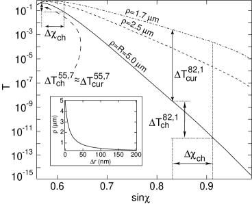
Figure 3: Transmission coefficient $T$ of a locally plane wave incident on a curved surface with the radii of curvature $\rho$ as a function of the incidence angle $\chi$ calculated from Eq. (46). The angle of total internal reflection $\sin\chi_{c}=0.56$ (corresponding to $n=1.8$). The inset shows the dependence of the average radius of local curvature due to boundary imperfections, $\rho$, subject to $\Delta r$ for the present model of surface roughness.

Figure 3 illustrates that $T$ decreases exponentially as the difference $\chi-\chi_{c}$ grows. The $Q$-value of the whispering gallery mode $q$ in a cavity of the radius $R$ is related to the transmission probability $T$, Eq. (46), by the relation Hentschel_rapid

$$Q=\frac{2nkR\cos\chi}{T},$$ (47)

where the classical incidence angle $\chi$ is related to mode number $q$ by Eq. (45), and $T\ll 1$.

III.2 Nonideal cavities with (a) surface roughness and (b) inhomogeneous refraction index

In this Section we present the results of numerical calculations of resonant states and $Q$-values of nonideal cavities. We consider separately two cases, (a), a disk cavity of a constant refraction index $n$ but with side wall imperfection (surface roughness), and, (b), a disk cavity of an ideal circular shape but with inhomogeneous refraction index $n=n(r,\varphi)$.

Various studies indicate that a typical size of the side-wall imperfections can vary in the range of 5-300 nm (representing a variation of the order of $\sim$0.05-1% of the cavity radius). Fujita ; Gayral ; Seassal ; Polson2002 . An exact experimental shape of the cavity-air interface is however not available. We thus model the interface shape as a superposition of random Gaussian deviations from an ideal circle of radius $R$ with a maximal amplitude $\Delta r/2$ and a characteristic distance between the deviation maxima $\Delta l\sim 2\pi R/50$. In a similar fashion we model the inhomogeneity of the diffraction index in the cavity, where a parameter $\Delta n$ characterizes a mean deviation of the refraction index $n$ from its average value $\langle n\rangle=1.8$. The variation of the refraction index $n$ can be caused by different factors including the presence of quantum well/wires/dots forming an active medium of the cavity, the local field intensity dependence $n=n(I)$, and other factors. Examples of typical structures under investigation are shown in Fig. 4.

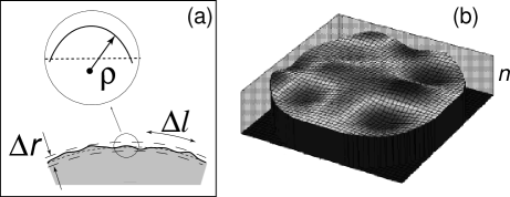
Figure 4: Examples of nonideal cavities studied in the present paper with (a) surface roughness and (b) inhomogeneous refraction index. (a) Radius of the disk $R=5\mu$m, $n=1.8$, surface roughness $\Delta r=100$ nm. (b) $R=5\mu$m, $\langle n\rangle=1.8$, $\Delta n=5\%$.

Figure 5 shows calculated $Q$-values of the disk resonant cavity for different surface roughnesses $\Delta r$ and the refraction index inhomogeneity $\Delta n$ in some representative wavelength interval. Note that we have studied a number of different resonances and all of them showed the same trends described below. Besides, here and hereafter we concentrate only on TM modes of the cavity, because TE modes exhibit similar features. The calculated dependencies of the $Q$-values on $\Delta r$ and $\Delta n$ are summarized in the insets to Fig. 5.

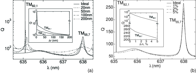
Figure 5: Dependencies $Q=Q(\lambda)$ for two representative modes TM_82,1 and TM_55,7 for the cases of (a) different surface roughness $\Delta r$ and (b) different refraction index inhomogeneities. The values of $\Delta r$ and $\Delta n$ are indicated in Figs. (a) and (b) respectively; $R=5\mu$m, $n=1.8$ (a), $\langle n\rangle=1.8$ (b). Note that in the case (b) the resonances shift when $\Delta n$ varies. For the sake of clearness we plot all the resonances centered around their maxima of the corresponding ideal disk (i. e. $\Delta n=0$). The broadening of the high-$Q$ resonance TM_55,7 is not discernible on the scale of the figure for all the values of $\Delta n$. Insets in Figs. (a) and (b) show the dependencies $Q=Q(\Delta r)$ and $Q=Q(\Delta n)$ respectively.

Let us first concentrate on the low-$Q$ state TM_55,7 ($q=55,m=7$). A decrease of the both surface roughness $\Delta r$ and the refractive index inhomogeneity $\Delta n$ causes graduate and rather slow decrease of the $Q$-value of this state as shown in the insets to Fig. 5. This behavior is typical for all other low-$Q$ states. In contrast, the high-$Q$ resonances exhibit very different and rather striking behavior. Namely, these resonances show a dramatic decrease of their $Q$-values even for very small values of the surface roughness $\Delta r\lesssim\lambda/50$. At the same time, the $Q$-values of the cavity decrease much more slowly when the refractive index inhomogeneity $\Delta n$ increases. For example, let us choose $\Delta r=20$nm and $\Delta n=5\%$. For these values of $\Delta r$ and $\Delta n$ the $Q$-value of the low-$Q$ state TM_55,7 drops by the same factor of $\sim 1.3$, decreasing from $Q\approx 270$ to $Q\approx 205$. In contrast, for the very same surface roughness $\Delta r$, the $Q$-value of a high-$Q$ state TM_82,1 drops by the factor of $\sim 10^{11}$ decreasing from its value $Q\approx 4\cdot 10^{13}$ for an ideal disk to $Q\approx 260$. At the same time, for the above value of $\Delta n=5\%$, the $Q$-value of this resonance decreases to the value of $Q\approx 1.3\cdot 10^{7}$, which corresponds to the drop by the factor $\sim 10^{4}$. (Note that for the case of an ideal cavity the high-$Q$ resonances are so narrow that the numerical resolution does not allow a reliable estimation of their exact values. In this case we therefore use Eq. (3) to estimate their $Q$-values.)

III.3 Discussion

In the previous Section we found that the surface roughness $\Delta r$ and refraction index inhomogeneity $\Delta n$ that produce similar degradation of low-$Q$ states, cause strikingly different effect on high-$Q$ resonances. In order to understand these features, we shall combine Poincaré surface of section and Husimi function methods with an analysis of ray reflection at a curved dielectric interface. The Poincaré surface of section (SoS) is a powerful tool visualizing the phase space for a classical ray dynamics in cavities Nockel ; Stone . We concentrate on the surface section of the phase space along the cavity boundary, $r\in\textrm{surf}$. For a given resonant state with an angular number $q$, the corresponding ray is launched with the angle $\chi_{0}=\arcsin\left(q/nkR\right)$ according to Eq. (45). Each reflection at the boundary (characterizing by the polar angle $\varphi$, and the angle of incidence $\chi$), corresponds to a single point in the plot. The number of bounces for a given angle of incidence $\chi_{0}$ is chosen in such a way that the total path of the ray does not exceed the one extracted from the numerically calculated $Q$-value for the corresponding resonance, $L=c\tau_{D}=Q/(kn)$. Figures 6 (a)-(c), (g)-(i) show a Poincaré surfaces of section (SoS) for the geometrical rays corresponding to the states TM_55,7, TM_82,1 for different values of the surface roughness $\Delta r$. For an ideal circular disk ($\Delta r=0$) the Poincaré SoS are obviously straight lines corresponding to a constant angle of incidence $\chi=\chi_{0}$. Figures 6 (b)-(c), (h)-(i) demonstrate that initially regular dynamics of an ideal cavity transforms into a chaotic one even for a cavity with maximum roughness $\Delta r\lesssim 20$nm. In Figs. 6 (b)-(c), (h)-(i) $\Delta\chi_{\textrm{ch}}$ approximately indicates the broadening of the phase space due to transition to the chaotic dynamics. An important observation is that for a given surface roughness $\Delta r$ the broadening of the phase space is independent of angular mode $q$, i.e. it is the same for low- and high-$Q$ states.

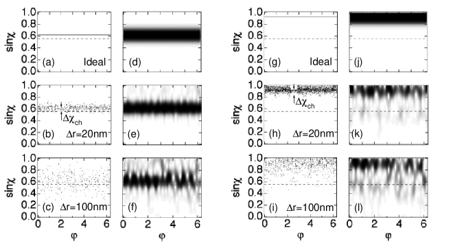
Figure 6: Poincaré surfaces of section for geometrical rays corresponding to the states $q=55$ (a)-(c) and $q=82$ (g)-(i) for the cavity with the surface roughness $\Delta r=0,20\textrm{nm},100\textrm{nm}$. The Husimi distributions for the states TM_55,7 (d)-(f) and TM_82,1 (j)-(l) for the same values of $\Delta r$ as in the corresponding Poincaré SoS. $\Delta\chi_{\textrm{ch}}$ indicate the broadening of the phase space due to transition to the chaotic dynamics. Dashed lines show the angle of total internal reflection $\chi_{c}$.

We complement classical Poincaré SoS by the Husimi function analysis Husimi ; Nockel ; Stone . The Husimi function (often called also Husimi distributions) $H(\varphi,\chi)$ represents a quantum (wave) analog to a classical Poincaré SoS. It is defined as a projection of a given cavity mode $\Psi{}(r\in\textrm{surf},\varphi)$ taken at the surface of cavity into a Gaussian wave packet $\Phi(\varphi^{\prime};\varphi,\chi)$ impinging the cavity boundary with the coordinate $\varphi$ at the angle $\chi$,

$$H(\varphi,\chi)=\int_{0}^{2\pi}{d\varphi^{\prime}\Psi(r\in\textrm{surf},\varphi^{\prime})\Phi(\varphi^{\prime};\varphi,\chi)},$$ (48)

where the minimum-uncertainty wave packet centered around $\varphi,\chi$ with the dispersion in position $\sqrt{\sigma/2}$ is given by

$$\Phi(\varphi^{\prime};\varphi,\chi)=(\pi\sigma)^{-\frac{1}{4}}\sum_{l}{\exp\left[{-\frac{1}{{2\sigma}}(\varphi^{\prime}-\varphi+2\pi l)^{2}-ik\sin\chi(\varphi+2\pi l)}\right]},$$ (49)

where we have chosen $\sigma=\sqrt{2}/k$. The Husimi distributions, Figs. 6 (d)-(f), (j)-(l), exhibit the same trends as the classical Poincaré SoS. Indeed, broadening the phase space with the increasing the surface roughness $\Delta r$ for the Husimi functions is the same as the corresponding broadening $\Delta\chi_{\textrm{ch}}$ in the Poincaré SoS. (Illustrative examples of the wave functions in cavities for different surface roughness $\Delta n$ are shown in Fig. 7).

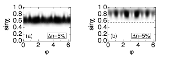
Figure 7: Illustrative examples of intensity distribution $E_{z}$ for the resonant state TM_55,7 in cavities with $\Delta r=0$ (a), $\Delta r=20\textrm{nm}$ (b), $\Delta r=20\textrm{nm}$ (c); $R=5\mu$m, $n=1.8$. Dashed lines indicate boundaries of the cavity.

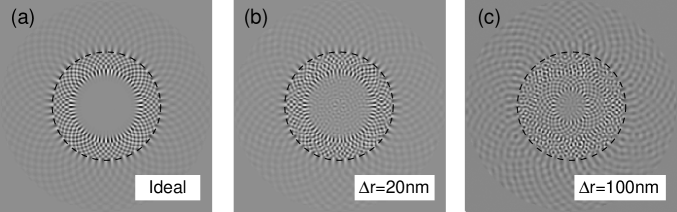
Figure 8: The Husimi distributions for the states TM_55,7 (a) and TM_82,1 (b) for the cavity with the refraction index inhomogeneity $\Delta n=5\%$.

Figure 8 shows the Husimi distributions for a circular cavity with an inhomogeneous refraction index. The variation of the refraction index $\Delta n=5\%$ is chosen in such a way that the degradation of the $Q$-value for the low-$Q$ resonance TM_55,7 is the same as the one for the case of surface roughness $\Delta r=20\textrm{nm}$ shown in Fig. 6. As expected, the broadening of the Husimi distribution due to increase of $\Delta n$ is of the same order as for the corresponding values $\Delta r$ (compare Figs. 6 and 8).

According to Eq (3), one can expect an increase of the transmission coefficient (and therefore decrease of the $Q$-value of the cavity) due to the broadening of the phase space $\Delta\chi_{\textrm{ch}}$, because the incidence angle $\chi$ effectively moves closer to the angle of the total internal reflection $\chi_{c}$. $\Delta T_{\textrm{ch}}$ in Fig. 3 indicates the estimated increase of the transmission coefficient due to the broadening of the phase space, $\Delta\chi_{\textrm{ch}}$, as extracted from the Poincaré SoS for the $\Delta r=20$nm and $\Delta n=5\%$. For the low-$Q$ resonance TM_55,7 this corresponds to the decrease of the $Q$-value by the factor of $\Delta Q_{\textrm{ch}}\sim\Delta T^{-1}_{\textrm{ch}}\approx 1.5$, which is consistent with the calculated decrease of the low-$Q$ resonances.

For the case of high-$Q$ resonance TM_82.1 the estimated decrease of the $Q$-factor is $\Delta Q_{\textrm{ch}}\sim\Delta T^{-1}_{\textrm{ch}}\approx 10^{3}\sim 10^{4}$ (see Fig. 3), which is consistent with the calculated decrease of this resonance for the case of the inhomogeneous refraction index only. (Note that because of a rather approximate definition of $\Delta\chi_{\textrm{ch}}$ we can give only very rough estimation of the factor $\Delta T_{\textrm{ch}}$.) On the contrary, for the case of high-$Q$ resonances in the presence of surface imperfections, this estimated value of $\Delta Q_{\textrm{ch}}$ is in many orders of magnitude smaller that the actual calculated decrease of the $Q$-factor (given by factor of $\approx 10^{11}$, see Fig. 5).

To explain the rapid degradation of high-$Q$ resonances, we concentrate on another aspect of the wave dynamics. Namely, the imperfections at the surface boundary effectively introduce a local radius of a surface curvature $\rho$ that is distinct from the disk radius $R$ (see illustration in Fig. 4). One may thus expect that with the presence of the local surface curvature, the total transmission coefficient will be determined by the averaged value of $\rho$ rather than by the disk radius $R$. The dependence of $\rho$ on surface roughness $\Delta r$ for the present model of surface imperfections is shown in the inset to Fig. 3. Figure 3 demonstrates that the reduction of the local radius of curvature from $5\mu$m (ideal disk) to $1.7\mu$m ($\Delta r=20$nm) causes an increase of the transmission coefficient by $\Delta T_{\textrm{cur}}\approx 10^{8}$. This estimate, combined with the estimate based on the change of $\Delta T_{\textrm{ch}}$ is fully consistent with the actual computed decrease of the $Q$-factor shown in Fig. 5. We thus conclude that the main mechanism responsible for the rapid degradation of high-$Q$ resonances in non-ideal cavities is the enhanced radiative decay through the curved surface because the effective local radius (given by the surface roughness) is smaller that the disk radius $R$.

In contrast, the degradation of low-$Q$ resonances (as well as high-$Q$ resonances in the case of inhomogeneous refraction index only), is mostly related to the broadening of the phase space caused by the transition to the chaotic dynamics. It should be noted however that both factors (broadening of the phase space and the enhancement of the transmission due to decrease of the effective radius of curvature) may play a comparable role in degradation of the low-$Q$ whispering-gallery resonances in the presence of surface roughness.

It is interesting to note that an analogues degradation of high-$Q$ modes was recently found in hexagonal-shaped microcavities, where the modes were strongly influenced by roundings of the corners even when the characteristic length scale (the local radius of curvature) was one order of magnitude smaller than the wavelength Wiersig_PRA . It is worth mentioning that one often assumes that long-lived high-$Q$ resonances in idealized cavities (e.g. in ideal disks, hexagons, etc.) are not important for potential application in optical communication or laser devicesHentschel ; Wiersig because of their extremely narrow width. Our simulations demonstrate that it is not the case, because in real structures the $Q$-values of these resonances becomes comparable to those of intermediate-$Q$ resonances already for small or moderate surface roughness of $\Delta r\sim 10-50$ nm.

IV Conclusions

In the present paper we develop a new, computationally effective, and numerically stable approach based on the scattering matrix ($S$-matrix) technique that is capable to deal with both arbitrary complex geometry and inhomogeneous refraction index inside the two-dimensional cavity. The derivation is based on the separation of the cavity region into $N$ narrow concentric rings and calculation of the $S$-matrix at every boundary between the rings. The total $S$-matrix is obtained in a recursive way by successive combination of the scattering matrixes for all the boundaries. In order to calculate the lifetime of the cavity modes (and, therefore their $Q$-factors) we compute the Wigner-Smith time delay-matrix which, in turn, is expressed in terms of the total scattering matrix.

We apply the developed algorithm to the calculation of resonant states and $Q$-values of nonideal microdisk cavities with (a) side wall imperfections and (b) circular cavities with inhomogeneous refraction index $n=n(r,\varphi)$. We find that the surface roughness $\Delta r$ and refraction index inhomogeneity $\Delta n$ that produce similar degradation of low-$Q$ states, cause strikingly different effect on high-$Q$ resonances. In particularly, in the case of inhomogeneous refraction index the increase of $\Delta n$ causes rather graduate decrease of the $Q$-value of high-$Q$ resonances. In contrast, in the presence of surface roughness even small imperfections ($\Delta r\lesssim\lambda/50$) can lead to a drastic degradation of high-$Q$ cavity modes by many orders of magnitude.

In order to understand these features, we combine Poincaré surface of section and Husimi function methods with an analysis of ray reflection at a curved dielectric interface. We argue that the main mechanism responsible for the rapid degradation of high-$Q$ resonances in non-ideal cavities with the surface roughness is the enhanced radiative decay through the curved surface because the effective local radius (given by the surface roughness) is smaller that the disk radius $R$. In contrast, the degradation of low-$Q$ resonances (as well as high-$Q$ resonances in the case of inhomogeneous refraction index only), is mostly related to the broadening of the phase space caused by the transition to the chaotic dynamics.

Appendix A Expressions for the matrixes $\mathbf{S^{i}}$

In this appendix we present the expressions for the matrixes $\mathbf{\Lambda},\mathbf{K},\mathbf{A},\mathbf{B}$ entering Eq. (43) for the scattering matrix $\mathbf{S^{i}}$ relating incoming and outgoing states at the $i$-th boundary. We distinguish three different cases as specified below.

(a) 0-th boundary (the boundary between the inner region ($i=0$) and the first ring $i=1$ in the intermediate region),

$$\mathbf{\Lambda_{11}}=\mathbf{I},\quad(\mathbf{\Lambda_{22}})_{mj}=e^{-\frac{1}{2}\Delta_{1}}\delta_{mj},\quad\mathbf{\Lambda_{12}}=\mathbf{\Lambda_{21}}=0,$$

$$\mathbf{K_{11}}=\mathbf{I},\quad(\mathbf{K_{22}})_{mj}=e^{i\gamma_{m}\Delta_{1}}\delta_{mj},\quad\mathbf{K_{12}}=\mathbf{K_{21}}=0,$$

$$\mathbf{A}=\left(\begin{array}[]{lcc}\mathbf{0}&\mathbf{V^{0,1}}\\ -\mathbf{J^{\prime}}&\mathbf{U^{0,1}P^{1}}\end{array}\right),\quad\mathbf{B}=\left(\begin{array}[]{cc}\mathbf{J}&-\mathbf{V^{0,1}}\\ \mathbf{0}&-\mathbf{U^{0,1}Q^{1}}\end{array}\right)$$

$$(\mathbf{J})_{mj}=J_{m}(n_{0}kd)\,\delta_{mj},\quad(\mathbf{J^{\prime}})_{mj}=J_{m}^{\prime}(n_{0}kd)\,\delta_{mj},$$

$$(\mathbf{V^{0,1}})_{mj}=\int_{0}^{2\pi}e^{-im\varphi}\Phi^{1}_{j}(\varphi)\,d\varphi,\quad(\mathbf{U^{0,1}})_{mj}=\frac{1}{n_{0}k\rho_{1}}\int_{0}^{2\pi}\frac{\chi_{0}^{2}(\varphi)}{\chi_{1}^{2}(\varphi)}e^{-im\varphi}\Phi^{1}_{j}(\varphi)\,d\varphi$$

(b) $i$-th boundary, $1<i<N-1$, (the boundary between $i$-th and $i+1$-th rings in the intermediate region)

$$(\mathbf{\Lambda_{11}})_{mj}=e^{\frac{1}{2}\Delta_{i}}\delta_{mj},\quad(\mathbf{\Lambda_{22}})_{mj}=e^{-\frac{1}{2}\Delta_{i+1}}\delta_{mj},\quad\mathbf{\Lambda_{12}}=\mathbf{\Lambda_{21}}=0,\quad(\mathbf{K})_{mj}=e^{i\gamma_{m}\Delta_{i}}\delta_{mj}\quad$$

$$\mathbf{A}=\left(\begin{array}[]{lcc}-\mathbf{I}&\mathbf{V^{i,i+1}}\\ -\mathbf{Q^{i}}&\mathbf{U^{i,i+1}P^{i+1}}\end{array}\right),\quad\mathbf{B}=\left(\begin{array}[]{cc}\mathbf{I}&-\mathbf{V^{i,i+1}}\\ \mathbf{P^{i}}&-\mathbf{U^{i,i+1}Q^{i+1}}\end{array}\right)$$

$$(\mathbf{V^{i,i+1}})_{mj}=\int_{0}^{2\pi}\left(\Phi^{i}_{m}(\varphi)\right)^{*}\Phi^{i+1}_{j}(\varphi)\,d\varphi,\quad(\mathbf{U^{i,i+1}})_{mj}=\frac{\rho_{i}}{\rho_{i+1}}\int_{0}^{2\pi}\frac{\chi_{i}^{2}(\varphi)}{\chi_{i+1}^{2}(\varphi)}\left(\Phi^{i}_{m}(\varphi)\right)^{*}\Phi^{i+1}_{j}(\varphi)\,d\varphi$$

(c) $N$-th boundary (the boundary between the last ring $i=N$ in the intermediate region and the outer region ($i=N+1$))

$$(\mathbf{\Lambda_{11}})_{mj}=e^{\frac{1}{2}\Delta_{N}}\delta_{mj},\quad\mathbf{\Lambda_{22}}=\mathbf{I},\quad\mathbf{\Lambda_{12}}=\mathbf{\Lambda_{21}}=0$$

$$(\mathbf{K_{11}})_{mj}=e^{i\gamma_{m}\Delta_{N}}\delta_{mj},\quad\mathbf{K_{22}}=\mathbf{I},\quad\mathbf{K_{12}}=\mathbf{K_{21}}=0,$$

$$\mathbf{A}=\left(\begin{array}[]{lcc}-\mathbf{I}&\mathbf{V^{N,N+1}H^{(1)}}\\ -\mathbf{Q^{N}}&\mathbf{U^{N,N+1}{H^{(1)}}^{\prime}}\end{array}\right),\quad\mathbf{B}=\left(\begin{array}[]{cc}\mathbf{I}&-\mathbf{V^{N,N+1}H^{(2)}}\\ \mathbf{P^{N}}&-\mathbf{U^{N,N+1}{H^{(2)}}^{\prime}}\end{array}\right)$$

$$(\mathbf{H^{(1,2)}})_{mj}=H^{(1,2)}(kR)\,\delta_{mj},\quad(\mathbf{{{H^{(1,2)}_{m}}^{\prime}}})_{mj}={{H^{(1,2)}_{m}}^{\prime}}(kR)\,\delta_{mj},$$

$$(\mathbf{V^{N,N+1}})_{mj}=\int_{0}^{2\pi}\left(\Phi^{N}_{m}(\varphi)\right)^{*}e^{ij\varphi}\,d\varphi,\quad(\mathbf{U^{N,N+1}})_{mj}=k\rho_{N}\int_{0}^{2\pi}\frac{\chi_{N}^{2}(\varphi)}{\chi_{N+1}^{2}(\varphi)}\left(\Phi^{1}_{j}(\varphi)\right)^{*}e^{ij\varphi}\,d\varphi$$

In Eqs. (A)-(A) the matrixes $\mathbf{Q^{i}},\mathbf{P^{i}}$ are defined according to

$$(\mathbf{P^{i}})_{mj}=\left(-\frac{1}{2}+i\gamma_{m}^{i}\right)\delta_{mj},\quad(\mathbf{Q^{i}})_{mj}=\left(-\frac{1}{2}-i\gamma_{m}^{i}\right)\delta_{mj},\quad 1\leq i\leq N.$$

${J_{m}},{H^{(1,2)}_{m}}$, and ${J_{m}}^{\prime},{H^{(1,2)}_{m}}^{\prime}$ are the Bessel and Hankel functions and their derivatives, and $\Delta_{i}=\Delta/\rho_{i}$.

References

- (1) Y. Yamamoto and R. E. Slusher, “Optical processes in microcavities”, Physics Today, June 1993, p.66.
- (2) J. U. Nöckel and R. K. Chang, “2-d microcavities: Theory and Experiments”, in Cavity-Enhanced Spectroscopies, R.D. van Zee and J.P.Looney, eds., (Vol. 40 of “Experimental Methods in the Physical Sciences”, Academic Press, San Diego, 2002), pp. 185-226.
- (3) S. C. Hill and R. E. Benner, “Morphology-dependent Resonances”, in Optical Effects Associated with Small Particles, P. W. Barber and R. K. Chang, eds. (Vol. 1 of “Advanced Series in Applied Physics”, World Scientific, Singapore, 1989).
- (4) S. L. McCall, A. F. J. Levi, R. E. Slusher, S. J. Pearton, and R. A. Logan, “Whispering-gallery mode microdisk lasers” Appl. Phys. Lett. 60, 289 (1992).
- (5) R. E. Slusher, A. F. J. Levi, U. Mohideen, S. L. McCall, S. J. Pearton, and R. A. Logan, “Threshold characteristics of semiconductor microdisk lasers”, Appl. Phys. Lett. 60, 289 (1992).
- (6) M. Fujita, K. Inoshita, and T. Bata, “Room temperature continuous wave lasing characteristics of GaInAsP/InP microdisk injection laser”, Electronic Lett., 34, 278-279 (1998).
- (7) B. Gayral, J. M. Gérard, A. Lemaître, C. Dupuis, L. Manin, and J. L. Pelouard, “High- wet etched GaAS microdisks containing InAs quantum boxes”, Appl. Phys. Lett. 75, 1908-1910 (1999).
- (8) C. Seassal, X. Letartre, J. Brault, M. Gendry, P. Pottier, P. Viktorovitch, O. Piquet, P. Blondy, D. Cros, O. Marty, “InAs wuantum wires in InP-based microdiscs: Mode identification and continuos wave room temperature laser operation”, J. Appl. Phys., 88, 6170-6174 (2000).
- (9) A. Dodabalapur, M. Berggren, R. E. Slusher, Z. Bao, A. Timko, P. Schiortino, E. Laskowski, H. E Katz, and O. Nalamasu, “Resonators and materials for organic lasers based on energy transfer” IEEE Journal of selected topics in quantum electronics, 4, 67-74 (1998).
- (10) M. Theander, T. Granlund, D. M. Johanson, A. Ruseckas, V. Sundström, M. R. Andersson, and O. Inganäs, “Lasing in a microcavity with an oriented liquid-crystalline polyfluorene copolymer as active layer”, Adv. Mater. 13, 323-37 (2001).
- (11) R. C. Polson, Z. Vardeny, and D. A. Chinn, “Multiple resonances in microdisk lasers of -conjugated polymers”, Appl. Phys. Lett. 81, 1561-1563 (2002).
- (12) K. S. Yee, “Numerical solution of initial boundary-value problems involving Maxwell’s equations in isotropic media”, IEEE Trans. Ant. Prop., AP-14, 302-307 (1996).
- (13) B.-J. Li and P.-L. Liu, “Analysis of far-field patterns of microdisk resonators by the finite-difference time-domain method”, IEEE J. Quantum Electron. 33, 1489 (1997).
- (14) M. N. O. Sadiku, Numerical Techniques in Electromagnetics, (CRC Press, Boca Raton, 2001).
- (15) P. C. Waterman, Symmetry, unitarity and geometry in electromagnetic scattering, Phys. Rev. D 3, 825-839 (1971).
- (16) M. I. Mishchenko, L. D. Travis, and A. A. Lacis, Scattering, Absorption, and Emission of Light by Small Particles, (Campridge University Press, Cambridge, 2002).
- (17) P. A. Knipp and T. L. Reinecke, “Boundary-element method for the calculation of the electronic states in semiconductor nanostructures”, Phys. Rev. B 54, 1880-1891 (1996).
- (18) J. Wiersig, J. Opt. A: Pure Appl. Opt. “Boundary element method for resonances in dielectric micrcavities”, 5, 53-60 (2003).
- (19) S. V. Boriskina, T. M. Benson, P. Sewell, and A. I. Nosich, “Highly efficient design of spectrally engineered whispering-gallery-mode microlaser resonators”, Opt. and Quant. Electr. 35, 545-559 (2003).
- (20) V. V. Nikolsky, T. I. Nikolskaya, Decomposition approach to the problems of electrodynamics (Nauka, Moskow, 1983), (in Russian).
- (21) S. Datta, Electronic Transport in Mesoscopic Systems (Cambridge University Press, Cambridge, 1995).
- (22) M. Hentschel and K. Richter, “Quantum chaos in optical system: The annular billiar”, Phys. Rev. E 66, 056207 1-13 (2002).
- (23) F. T. Smith, “Lifetime matrix in collision theory”, Phys. Rev, 118, 349 (1960).
- (24) M. Bauer, P. A. Mello, and K. W. McVoy, “Time delay in nuclear reactions”, Z. Physik A 293, 151 (1979).
- (25) Z. S. Wu and Y. P. Y. Wang, “Electromagnetic scattering for multilayered sphere: recursive algorithms”, Radio Sci. 26, 1393-1401 (1991).
- (26) B. R. Johnson, “Light scattering by a multilayer sphere”, Applied Optics 35, 3286-3296 (1996).
- (27) A. V. Snyder and J. D. Love, “Reflection at a curved dielectric interface – Electromagnetic tunneling”,IEEE Trans. Microwave. Theor. Techn. MTT-23, 134-141 (1975).
- (28) M. Hentschel and H. Schomerus, “Fresnel laws at curved dielectric interfaces of microresonators”, Phys. Rev. E. 65, 045603 1-4 (R) (2002).
- (29) A. D. Stone, “Wave-chaotic optical resonators and lasers”, Physica Scripta T90, 448 (2001) (Proceedings of the Nobel Symposium ”Quantum Chaos 2000”).
- (30) B. Crespi, G. Perez, and S. J. Chang, “Quantum Poincaré sections for two-dimentional billiards”, Phys. Rev. E 47, 986-991 (1993).
- (31) J. Wiersig, private communication; J. Wiersig, “Hexagonal dielectric resonators and microcrystal lasers”, Phys. Rev. A 67 023807 1-12 (2003).