Scaling laws in the functional content of genomes

With the number of sequenced genomes now over one hundred, and the availability of rough functional annotations for a substantial proportion of their genes, it has become possible to study the statistics of gene content across genomes. Here I show that, for many high-level functional categories, the number of genes in the category scales as a power-law in the total number of genes in the genome. The occurrence of such scaling laws can be explained with a simple theoretical model, and this model suggests that the exponents of the observed scaling laws correspond to universal constants of the evolutionary process. I discuss some consequences of these scaling laws for our understanding of organism design.

What fraction of a genome’s gene content is allotted to different functional tasks, and how does this depend on the complexity of the organism? Until recently, there was simply no data to address such questions in a quantitative way. Presently, however, there are more than $100$ sequenced genomes [7] in public databases, and protein-family classification algorithms allow functional annotations for a considerable fraction of the genes in each genome. Thus, it has become possible to analyze the statistics of functional gene-content across different genomes, and here I present results on the dependency of the number of genes in different high-level categories on the total number of genes in the genome.

Evaluating the functional gene-content of genomes

To estimate the number of genes in different functional categories each genome has to be functionally annotated. The main results presented in this paper were obtained using the Interpro [1] annotations of sequenced genomes available from the European Bioinformatics Institute [2]. To map the Interpro annotations to high-level functional categories I used the Gene Ontology “biological process” hierarchy [3] and a mapping from Interpro entries to GO-categories both of which can be obtained from the gene ontology website [4]. For each GO category I collect all Interpro entries that map to it or to one of its descendants in the “biological process” hierarchy. To minimize the effects of potential biases in the mappings from Interpro to GO I only use high-level functional categories that are represented by at least $50$ different Interpro entries. This leaves $44$ high-level GO categories.

A gene with multiple hits to Interpro entries that are associated with a GO category has a higher probability to belong to that category than a gene with only a single hit. To take this information into account, I assume that if a gene $i$ has $n^{c}_{i}$ independent hits to Interpro entries associated with GO category $c$, than with probability $1-\exp(-\beta n^{c}_{i})$ the gene belongs to the GO category. The results are generally insensitive to the value of $\beta$ (see the appendix), and I used $\beta=3$ for the results shown below. The estimated number of genes $n_{c}$ in a genome for a given GO category is then the sum $n_{c}=\sum_{i}1-\exp(-\beta n^{c}_{i})$ over all genes $i$ in the genome.

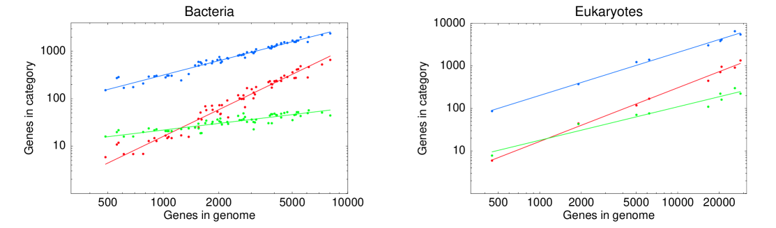
Figure 1: The number of transcription regulatory genes (red), metabolic genes (blue), and cell cycle related genes (green) as a function of the total number of genes in the genome for bacteria (A) and eukaryotes (B). Both axes are shown on logarithmic scales. Each dot corresponds to a genome. The straight lines are power-law fits. Archaea are not shown because the range of genome sizes in archaea is too small for meaningful fits. For completeness the archaeal results are shown in figure 3 in the appendix.

Figure 1 shows the results for the categories of transcription regulatory genes (red), metabolic genes (blue), and cell-cycle related genes (green) for bacteria (panel A) and eukaryotes (panel B). Remarkably, for each functional category shown, we find an approximately power-law relationship (solid line fits). That is, if $n_{c}$ is the number of genes in the category, and $g$ is the total number of genes in the genome, we observe laws of the form: $n_{c}=\lambda g^{\alpha}$, where both $\lambda$ and the exponent $\alpha$ depend on the category under study. In fact, such power-laws are observed for most of the $44$ high-level categories, and the estimated values of the exponents for several functional categories are shown in Table 1. Note that a potential source of bias in estimating these exponents is the occurrence of multiple genomes from the same or closely-related species in the data. As shown in the appendix, removing this “redundancy” from the data does not alter the observed exponents.

Table 1: Estimates for the exponents of a selection of functional categories. The first number gives the maximum likelihood estimate of the exponent while the second indicates the boundaries of the $99$% posterior probability interval.

The power-law fits and $99$% posterior probability estimates for their exponents were obtained using a Bayesian procedure described in the appendix. To assess the quality of the fits, I measured, for each fit, the fraction of the variance in the data that is explained by the fit. In bacteria, $26$ out of $44$ GO categories have more than $95$% of the variance explained by the fit, $38$ categories have more than $90$% explained. In eukaryotes, $26$ categories have more than $95$% percent explained by the fit and $32$ have more than $90$% explained by the fit. However, with total gene number varying over less than two decades in bacteria, and the small number of data points in eukaryotes, one may wonder how one can claim that power-laws have been “observed”. First, the fact that I fit the data to power-laws should not be mistaken for a claim that the data can only be described by power-law functions. I only claim that the power-law is by far the simplest functional form that fits almost all the observed data. Second, when scatter plots such as those shown in Fig. 1 are plotted on linear as opposed to logarithmic scales, it is clear even by eye that the fluctuations in the number of genes in a category scale with the total number of genes in the genome. That is, the fluctuations in the data suggest that logarithmic scales are the “natural” scales for this data. This is further supported by the simple evolutionary model presented below.

One may also wonder to what extent the results are sensitive to the specific functional annotation procedure. I performed a variety of tests to assess the robustness of the results, i.e. the observed power-law scaling and the values of the exponents, to changes in the annotation methodology (see appendix). These involve using entirely independent annotations based on Clusters of Orthologous Groups of proteins (COG) [10], and a simple (crude) annotation scheme based on keyword searches of protein tables for sequenced microbial genomes from the NCBI website [8]. As shown in the appendix, the observed power-law scaling, and the values of the exponents are generally insensitive to these and other changes in annotation methodology. It has to be noted, however, that all currently available annotation schemes, including the ones used here, predict function from sequence homology and thus at some level assume that functional homology can be inferred from sequence homology. The results reported here thus also depend on this assumption.

Observed Exponents

Some functional categories, such as the large category of metabolic genes, occupy a roughly constant fraction of a genome’s gene-content, as evidenced by their exponent of $1$. However, many categories show significant deviations from this “trivial” exponent. Genes related to cell-cycle or protein biosynthesis have exponents significantly below $1$, whereas for transcription factors (TFs) the exponent is significantly above $1$. These trends are strongest in bacteria. There the exponent for TFs is almost $2$, implying that as the number of genes in the genome doubles, the number of TFs quadruples. This has some interesting implications for “regulatory design” in bacteria. It implies that the number of TFs per gene grows in proportion to the size of the genome (see [9] for a similar observation). This in turn implies that, in larger genomes, each gene must be regulated by a larger number of TFs and/or each TF must be regulating a smaller set of genes. An exponent of $2$ is also observed for two-component systems, which are the primary means by which bacteria sense their environment. This suggests that the relative increase in transcription regulators in more complex bacteria is accompanied by an equal relative increase in sensory systems.

The difficulties with gene prediction and annotation in eukaryotes, the small number of available genomes, and our lack of understanding of the role of alternative splicing across eukaryotic genomes make it premature to draw many conclusions from Fig. 1B. However, the main trends from Fig. 1A are reproduced: the super linear scaling of TFs, the sub linear scaling of cell-cycle genes, and the small exponents for DNA replication and protein biosynthesis genes.

The observed super linear scaling of TFs also has implications for our understanding of “combinatorial control” in transcription regulation. It is well established that in complex organisms, different TFs combine into complexes to affect transcription control. Therefore, a relatively small number of TFs can implement a combinatorially large number of different transcription regulatory “states”, which may correspond to particular external environments, developmental stages, tissues, combinations of external stimuli, etcetera. Each such regulatory state will be associated with a unique set of genes that are expressed in that state. If the number of such regulatory states were proportional to the total number of genes, then the number of TFs would increase much more slowly than the total number of genes. However, the scaling results show that, instead, the number of TFs increases more rapidly than the total number of genes. This thus implies that the number of regulatory states is also “combinatorial” in the total number of genes: a relatively small number of genes is used in different combinations to implement combinatorially many regulatory states.

The picture that emerges is not of TFs being used in different combinations to implement the regulatory needs of individual genes. But rather that, as one moves from simple to more complex organisms, the number of regulatory states grows so much faster than the total number of genes that, even with combinatorial control of transcription, the number of TFs grows much faster than the total number genes.

Evolutionary model

One of course wonders about the origins of these scaling laws in genome organization, and I like to present some speculations in this regard. Assume that most changes in the number of genes $n_{c}$ in a functional category $c$ are caused by duplications and deletions. Then, $n_{c}(t)$ generally evolves according to the equation

$$\frac{dn_{c}(t)}{dt}=(\beta(t)-\delta(t))n_{c}(t)=\rho(t)n_{c}(t),$$ (1)

with $\beta(t)$ and $\delta(t)$ respectively the duplication- and deletion-rate of the genes in this category at time $t$ in the evolutionary history of the genome. For simplicity of notation I have introduced the difference of duplication and deletion rates $\rho(t)$, which can be thought of as an “effective” duplication rate. This rate $\rho(t)$ is presumably proportional to the difference between the average probability that selection will favor fixation of a duplicated gene from this category and the average probability that selection will favor deletion of a gene from this category. Similarly, the total number of genes $g(t)$ obeys the equation

$$\frac{dg(t)}{dt}=\gamma(t)g(t),$$ (2)

with $\gamma(t)$ the overall effective rate of gene duplication in the genome at time $t$ in its evolutionary history. When we solve for $n_{c}$ as a function of $g$ we find

$$n_{c}=\lambda g^{\langle\rho\rangle/\langle\gamma\rangle},$$ (3)

where $\langle\rho\rangle$ and $\langle\gamma\rangle$ are the mean effective duplication rates of genes in category $c$ and the entire genome respectively, averaged over the evolutionary history of the genome, and $\lambda$ is a constant that depends on the boundary conditions. In order for all bacterial genomes to obey the same functional relation, the constant $\lambda$ and the ratios $\langle\rho\rangle/\langle\gamma\rangle$ have to be the same for all bacterial evolutionary lineages. Since all life shares a common ancestor, the boundary conditions for equations (1) and (2) are trivially the same for all bacterial lineages, implying that the constant $\lambda$ is indeed the same for all bacterial lineages. In summary, simply assuming that changes in gene-number occur mostly through duplications and deletions implies our observed power-law scaling if the ratios $\langle\rho\rangle/\langle\gamma\rangle$ are the same for all evolutionary lineages.

I thus propose that the explanation for the observed scaling-laws is that the ratios $\langle\rho\rangle/\langle\gamma\rangle$ are indeed the same for all bacterial lineages, i.e. these ratios of average duplication rates are “universal constants” of genome evolution. For instance, the exponent $2$ for TFs in bacteria indicates that, in all bacterial lineages, evolution selects duplicated TFs twice as frequently as duplicated genes in general. It seems likely that such universal constants are intimately connected to fundamental design principles of the evolutionary process. It is tempting to become even more speculative in this regard, and suggest that this factor of $2$ in duplication rate is related to switch-like function of transcription factors: with each addition of a transcription factor the number of transcription-regulatory states of the cell doubles. It is not entirely implausible to assume that with twice the number of internal states available, the probability of such a duplication being fixed in evolution is twice as large as the probability of fixing a duplicated gene that does not double the number of internal states of the cell.

Finally, as table 1 shows, there is still substantial uncertainty about the exact numerical values of the exponents given the current data, and many more genomes are needed to estimate these values more accurately. A survey of the NCBI genome database [7] shows that the number of sequenced genomes is increasing exponentially, with a doubling time of about $16$ months (Fig. 2).

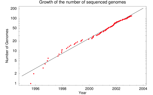
Figure 2: The number of fully-sequenced genomes in the NCBI database [7] as a function of time. The vertical axis is shown on a logarithmic scale. The straight line is a least squares fit to an exponential function: $n(t)=2^{(t-1994)/1.3}$.

This suggests that within a few years thousands of genomes will become available. With such an increase in available data it will become possible to look at much more fine-grained gene content statistics than the ones presented here. One can for instance imagine going beyond looking at single functional categories at a time, and investigate if there are correlations in the variations of gene number in more fine-grained functional categories. I believe that such investigations have the potential to teach us much about the functional design principles of the evolutionary process.

Appendix

Results for Archaea

Figure 3 shows the number of transcription regulatory genes (red), metabolic genes (blue), and cell-cycle related genes (green) as a function of the total number of genes in archaeal genomes.

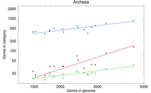
Figure 3: The number of transcription regulatory genes (red), metabolic genes (blue), and cell cycle related genes (green) as a function of the total number of genes in archaea. Both axes are shown on logarithmic scales. Each dot corresponds to a genome. The straight lines are power-law fits.

Note that the size of the largest archaeal genome differs from that of the smallest by only a factor of approximately $3$. Consequently, there is large uncertainty regarding the values of the exponents for archaea. The maximum likelihood values and $99$% posterior probability intervals are $2.1$ and $[1.3-5.7]$ for transcription regulatory genes, $0.81$ and $[0.44-1.48]$ for metabolic genes, and $0.83$ and $[0.54-1.35]$ for cell-cycle related genes.

Power-law Fitting

The power-law fits in figure 1 were obtained using a Bayesian straight-line fitting procedure. For each GO-category, I log-transform the data such that each data point $(x_{i},y_{i})$ corresponds to the logarithm of the estimated total number of genes, and the logarithm of the estimated number of genes in the category respectively. I assume that these transformed data where drawn from a linear model

$$y=\alpha(x+\epsilon)+\lambda+\eta,$$

where $\eta$ and $\epsilon$ are “noise” terms in the $x$- and $y$-coordinates respectively and $\lambda$ in an unknown off-set. I assume that the joint-distribution $P(\eta,\epsilon)$ is a two-dimensional Gaussian with means zero and unknown variances and co-variance. That is, I use scale invariant priors for the variances, and will integrate these nuisance variables out of the likelihood. A uniform prior is used for the location parameter $\lambda$, and for the slope $\alpha$ I will use a rotation invariant prior:

$$P(\alpha)d\alpha=\frac{d\alpha}{(1+\alpha^{2})^{3/2}}.$$

The use of these priors guarantees that the results are invariant under all shifts and rotations of the plane.

Integrating over all variables except for $\alpha$, we obtain for the posterior $P(\alpha|D)$ given the data $D$:

$$P(\alpha|D)d\alpha=C\frac{(\alpha^{2}+1)^{(n-3)/2}d\alpha}{(\alpha^{2}s_{xx}-2\alpha s_{yx}+s_{yy})^{(n-1)/2}},$$

where $n$ is the number of genomes in the data, $s_{xx}$ is the variance in $x$-values (logarithms of the total gene numbers), $s_{yy}$ the variance in $y$-values (logarithms of the number of genes in the category), $s_{yx}$ is the co-variance, and $C$ is a normalizing constant. The values of the exponents reported in table 1 are the values of $\alpha$ that maximize $P(\alpha|D)$, and the boundaries of the $99$% posterior probability interval around it.

For each fit, I also measure what fraction of the variance in the data is explained by the fit. That is, I compare the average distance $d$ of the points in the plane to their center of mass with the average distance $d_{l}$ of the points to the fitted line and define the fraction $q=1-d_{l}/d$ as the variance in the data explained by the fit.

Robustness of the results

I first checked that the total amount of available annotation information is not itself dependent on genome size. If the total amount of available annotation information were to vary with the number of genes in the genome, this could lead to biases in the estimated exponents. To exclude this possibility, I counted the total number of genes with any Interpro hits in each genome and found that, for both bacteria and eukaryotes, the fraction of genes in the genome with Interpro hits is about $2/3$, independent of the total number of genes in the genome. Consistent with this observation, when one fits power-laws to the number of genes $n_{c}$ in a GO-category $c$ as a function of the total number of annotated genes in the genome, one finds exponents that are very close to those founds for $n_{c}$ as a function of the total number of genes in the genome.

Second, I tested that the results are insensitive to the value of the parameter $\beta$. The default value $\beta=3$ gives a gene with a single Interpro hit a probability of $1-e^{-3}\approx 0.95$ to belong to the category. This is reasonable because Interpro is designed to only report statistically significant hits. To assess the effect of changing $\beta$, results for $\beta=1$ were generated. For bacteria the change in fitted exponent is less than $5$% for $26$ of $44$ categories, and less than $10$% for $39$ categories. For eukaryotes the exponent changes by less than $5$% for all but $3$ categories. In all cases, the change in fitted exponent is significantly smaller than the $99$% posterior probability intervals associated with the exponents of the fits.

Third, I tested the robustness of the results against removal of potential “redundancies” in the data. For bacteria there are several examples where multiple genomes of the same species or genomes of very closely related species occur in the data, and one might suspect that these may bias the results in some way. To this end, I parsed the names of all bacterial species into a general and a specific part, e.g. for Escherichia Coli Escherichia is the general part and coli the specific part, for Listeria innocua Listeria is the general part and innocua the specific part, etcetera. Groups of genomes with the same general part were then collected together and for each group the gene numbers were replaced with a single average of total gene number and average gene counts in each of the functional categories. This reduces the size of the data set by about a third. Power-law fitting was then applied to this reduced set and the fitted exponents were compared with those of the full data set. The maximum likelihood exponent was changed by less than $5$% in $31$ out of $44$ categories. The largest observed change was an $18$% change in the exponent. All changes to the exponents were well within the $99$% posterior probability intervals.

More importantly, the results could depend on the use of Interpro, the Gene Ontology, and the mapping of Interpro entries to GO categories. To test the robustness of the results to biases inherent in Interpro annotation and/or the mapping from Interpro to Gene Ontology, I analyzed selected functional categories using two other annotation schemes.

The first is based on Clusters of Orthologous Groups of proteins (COG) [10] annotation of $63$ bacterial genomes that can be obtained from
ftp://ftp.ncbi.nih.gov/pub/COG/COG.
In this data set, proteins of the $63$ bacterial genomes are assigned to COGs, and the COGs have been assigned to functional categories. I used these assignments to count the number of genes in different functional categories according to the COG annotation scheme. A comparison of the exponents for COG functional categories and the exponents for the closest GO categories obtained using the Interpro annotations are shown in table 2.

The second alternative annotation scheme I used is based on simple keyword searches of protein tables for fully-sequenced bacterial genomes available from the NCBI ftp site:
ftp.ncbi.nlm.nih.gov/genomes/Bacteria.
Removing genomes for which little or no annotation exists, this leaves protein tables for $90$ bacterial genomes. Each protein in these protein tables is annotated with a short description line. The number of genes in different functional categories was counted by searching each description line for hits to a set of keywords that characterize the category. For instance, I chose the keywords “ribosom”, “translation”, and “tRNA” for the category “protein biosynthesis”, and the gene is counted as belonging to this category if any of these keywords occurs in its description line. For the other categories I used the following keywords: “transcription” for the category “transcription”; “transport”, “channel”, “efflux”, “pump”, “porin”, “export”, “permease”, “symport”, “transloca”, and “PTS” for the category “transport”; all combinations “X Y” with X being one of “ion”, “sodium”, “calcium”, “potassium”, “magnesium”, and “manganese”, and Y being one of “channel”, “efflux”, “transport”, and “uptake” for the category “ion transport”; ‘protease” and “peptidase” for the category “protein degradation”; “kinase” for the category “kinase”; and finally the phrases ‘DNA polymerase”, “topoisomerase”, “DNA gyrase”, “DNA ligase”, “replication”, “helicase”, “DNA primase”, “DNA repair”, “cell division”, and “septum” for the category “cell cycle”. The exponents resulting from this (crude) annotation scheme are also shown in table 2. As table 2 shows, there is good quantitative agreement between the exponents that are obtained with the different annotation schemes.

Table 2: Estimated $99$% posterior probability intervals for the scaling exponents obtained with three different annotation schemes.

Annotation	Category	Exponent
GO	Protein biosynthesis	0.11-0.15
COG	Translation, ribosomal structure and biogenesis	0.21-0.37
NCBI	Protein biosynthesis	0.09-0.15
GO	Signal transduction	1.55-1.9
COG	Signal transduction mechanisms	1.66-2.14
GO	Protein metabolism and modification	0.68-0.8
GO	Protein degradation	0.89-1.06
COG	Posttranslational modification, protein turnover, chaperones	0.88-1.15
NCBI	Protein degradation	0.68-0.91
GO	Cell cycle	0.39-0.54
GO	DNA repair	0.52-1.14
COG	Replication, recombination and repair	0.66-0.83
NCBI	Cell cycle	0.45-0.64
GO	Ion transport	1.15-1.7
COG	Inorganic ion transport and metabolism	1.19-1.47
NCBI	Ion transport	1.12-1.88
GO	Regulation of transcription	1.74-2
COG	Transcription regulation	1.69-2.36
NCBI	Transcription	1.9-2.42
GO	Kinase	0.96-1.16
NCBI	Kinase	0.8-1.03
GO	Transport	1.08-1.32
NCBI	Transport	1.16-1.5

References

- [1] R. Apweiler, T. K. Attwood, A. Bairoch, A. Bateman, E. Birney, M. Biswas, P. Bucher, L. Cerutti, F. Corpet, M. D. Croning, R. Durbin, L. Falquet, W. Fleischmann, J. Gouzy, H. Hermjakob, N. Hulo, I. Jonassen, D. Kahn, A. Kanapin, Y. Karavidopoulou, R. Lopez, B. Marx, N. J. Mulder, M. Oinn, M. Pagni, F. Servant, C. J. Sigrist, and E. M. Zdobno. The interpro database, an integrated documentation resource for protein families, domains and functional sites. Nucleic Acids Res., 29(1):37–40, 2001.
- [2] R. Apweiler, M. Biswas, W. Fleischmann, A. Kanapin, Y. Karavidopoulou, P. Kersey, E. V. Kriventseva, V. Mittard, N. Mulder, I. Phan, and E. Zdobnov. Proteome analysis database: online application of interpro and clustr for the functional classification of proteins in whole genomes. Nucleic Acids Res., 29(1):44–48, 2001.
- [3] The Gene Ontology Consortium. Gene ontology: tool for the unification of biology. Nature Genetics, 25:25–29, 2000.
- [4] http://www.geneontology.org.
- [5] M. Huynen and E. van Nimwegen. The frequency distribution of gene family sizes in complete genomes. Mol. Biol. Evol., 15(5):583–589, 1998.
- [6] N. M. Luscombe, J. Qian, Z. Zhang, T. Johnson, and M. Gerstein. The dominance of the population by a selected few: power-law behavior applies to a wide variety of genomic properties. Genome biology, 3(8), 2002.
- [7] http://www.ncbi.nlm.nih.gov/genomes/index.htm.
- [8] ftp.ncbi.nlm.nih.gov/genomes/bacteria.
- [9] C. K. Stover, X. Q. T Pham, A. L. Erwin, S. D. Mizoguchi, P. Warrener, M. J. Hickey, F. S. L. Brinkman, W. O. Hufnagle, D. J. Kowalik, M. Lagrou, R. L. Garber, L. Goltry, E. Tolentino, S. Westbrook-Wadman, Y. Yuan, L. L. Brody, S. N. Coulter, K. R. Folger, A. Kas, K. Larbig, R. M. Lim, K. A. Smith, D.H. D. H. Spencer, G. K.-S. Wong, Z. Wu, I. T. Paulsen, J. Reizer, M. H. Saier, R. E. W. Hancock, S. Lor, and M. V. Olson. Complete genome sequence of pseudomonas aeruginosa pa01, an opportunistic pathogen. Nature, 406:959–964, 2000.
- [10] R. L. Tatusov, E. V. Koonin, and D. J. Lipman. A genomic perspective on protein families. Science, 278:631–637, 1997.