Nuclear mass systematics using neural networks

Abstract

New global statistical models of nuclidic (atomic) masses based on multilayered feedforward networks are developed. One goal of such studies is to determine how well the existing data, and only the data, determines the mapping from the proton and neutron numbers to the mass of the nuclear ground state. Another is to provide reliable predictive models that can be used to forecast mass values away from the valley of stability. Our study focuses mainly on the former goal and achieves substantial improvement over previous neural-network models of the mass table by using improved schemes for coding and training. The results suggest that with further development this approach may provide a valuable complement to conventional global models.

,

1 Introduction

The problem of devising global models of nuclidic (atomic) masses has a long history, going back to the early work of Bohr, von Weizsäcker and Bethe based on the liquid drop model (see refs. [1, 2, 3, 4, 5, 6] for reviews). The principal objectives are (i) a fundamental understanding of the physics of the mass surface and (ii) the prediction of the masses of “new” nuclides far from stability, both in the superheavy region and in the regions approaching the proton and neutron drip lines.

The actual predictions for the masses are of great current interest in connection with present and future experimental studies of nuclei far from stability, conducted at heavy-ion and radioactive ion-beam facilities [7]. The results are also useful for such astrophysical problems as nucleosynthesis and supernova explosions. The spectrum of models of the atomic mass table ranges from those with high theoretical input that take explicit account of known physical principles in terms of a relatively small number of fitting parameters, to models that are shaped mostly by the data and very little by theory and thus have a correspondingly larger number of adjustable parameters. Epitomizing models of the former class are the macroscopic/microscopic models of Möller, Nix, and coworkers [1, 8, 9, 10], and the semi-microscopic models of Pearson, Tondeur, and coworkers [11, 12, 13]. The models of Möller et al. appeal to the macroscopic descriptions provided by the liquid drop and droplet models, solve a one-body Schrödinger equation to incorporate single-particle degrees of freedom, and include pairing through semi-microscopic calculation. A prominent version, which sets the standard for state-of-the-art theory-based models, is the finite-range droplet model (FRDM) detailed in ref. [10]. The models of Pearson, Tondeur, and coworkers are based on the Hartree-Fock method, with pairing correlations described by either a BCS or Bogolyubov treatment. The current version, namely the HFB2 model [13], features the Bogoliubov approach and an improved Skyrme force.

In this work we use neural networks to develop global nuclear mass models which are situated far toward the other end of the spectrum, where one (in the ideal) seeks to determine the degree to which the entire mass table is determined by the existing experimental data, and only the data. During the last decade, artificial neural networks have been utilized to construct predictive statistical models in a variety of scientific problems ranging from astronomy to experimental high-energy physics to protein structure [14, 15]. In a typical application, a multilayer feedforward neural network is trained with back-propagation or some other supervised training algorithms [16, 17, 18, 19] so as to create a “predictive” statistical model of a certain input-output mapping, which may in general be physical or mathematical in character. Information contained in a set of learning examples of the input-output association is embedded in the weights of the connections between the layered units. This information may (or may not) be sufficient to allow the trained network to make reliable predictions for examples outside the learning set. At any rate, the network is taught to generalize (well or poorly), based on what it has learned from the set of examples. In the more mundane language of function approximation, the neural-network model provides a means for interpolation or extrapolation.

Nuclear physics offers especially rich territory for “data mining” with neural nets. On the one hand, a huge collection of high-quality experimental data is available for diverse properties of more than 2000 nuclides. On the other, quantitative calculation of some properties of some classes of nuclei presents difficult challenges even for the best ab initio quantum-mechanical theories and phenomenological macroscopic/microscopic models. To date, global neural-network models have been developed for the stability/instability dichotomy, for the atomic-mass table, for neutron separation energies, for spins and parities, for decay branching probabilities of nuclear ground states, and for $\beta$ decay half-lives [20, 21, 22, 23, 24, 25, 26, 27, 28, 29, 30].

In the work to be described here, neural nets have been trained to predict the nuclear mass excess or “defect” $\Delta M$, continuing the program established in refs. [20, 21, 23, 28, 29]. In Sec. 2, we outline the training methodology that has been applied and specify the data sets used in the modeling process. The results are presented and discussed in Sec. 3. Finally, Sec. 4 states the general conclusions of the current study and views the prospects for further successes and further improvements in statistical prediction of atomic masses.

2 Design and training of neural-network models

Our immediate tasks are to specify (i) the structure and unit-dynamics of the networks that will be developed to model the mass data and (ii) the algorithm for their training. We must also specify (iii) the data sets to be utilized together with (iv) the schemes for encoding and decoding input and output data.

2.1 Architecture and Dynamics

A multilayer feedforward architecture is adopted, with various numbers of hidden layers and distributions of units among layers. The gross architecture of a given net is summarized in the notation ($I$–$H_{1}$–$H_{2}$–…–$H_{L}$–$O$)[$P$], where $P$ is the total number of weight/bias parameters and $I$, $H_{i}$, and $O$ are integers that indicate, respectively, the numbers of neuron-like units in the input layer, the $i$th intermediate (or “hidden”) layer, and the output layer. Unless otherwise indicated, each unit in a layer is connected to all units to the next layer. The connection from unit $m$ to unit $n$ is characterized by a real-number weight $w_{mn}$ with initial value positioned at random in the range $[-1,1]$.

When a pattern $\mu$ is impressed on the input interface, the activities of the input units are set in accordance to the coding scheme assumed (see section 2.4.). Each unit in a hidden layer or in the output layer receives a stimulus $u_{n}=\sum_{m}w_{mn}a_{m}$, where the $a_{m}$ are the activities of the units in the immediately preceding layer. The activity of generic unit $m$ in the hidden or output layers is in general a nonlinear function of its stimulus, $a_{m}=g(u_{m})$. In our work, the activation function $g(u)$ is taken to have the logistic form, $g(u)=\bigl{[}1+\exp(-u)\bigr{]}^{-1}$. The system response may be decoded from the activities of the units of the output layer also in accordance to the coding scheme assumed. The dynamics is particularly simple: the states of all units within a given layer are updated in parallel and the layers are updated successively, proceeding from input to output.

2.2 Training Algorithms

Several training algorithms exist that seek to minimize the cost function with respect to the network weights. For the cost function we make the traditional choice of the sum of squared errors calculated over the learning set, or more specifically

$$E=\sum_{\mu}E^{(\mu)}=\frac{1}{2}\sum_{{\mu},i}(t_{i}^{(\mu)}-o_{i}^{(\mu)})^{2}\,,$$ (1)

where $t_{i}^{(\mu)}$ and $o_{i}^{(\mu)}$ denote, respectively, the target and actual activities of unit $i$ of the output layer for input pattern (or example) $\mu$. In global modeling of the atomic mass table, the root-mean-square error $\sigma_{\mathrm{r}ms}$ has been widely adopted as the key figure of merit, and we shall use its value, calculated over various data sets, to assess the performance of neural-network models. When evaluated over the learning set, this quantity evidently coincides with $(2E/N_{p})^{1/2}$, where $N_{p}$ is the number of training examples.

The most familiar training algorithm is standard back-propagation [16, 18] (hereafter often denoted SB), according to which the weight update rule to be implemented upon presentation of pattern $\mu$ is

$$\Delta w_{mn}^{(\mu)}=-\eta\frac{\partial E^{(\mu)}}{\partial w_{mn}}+\alpha\Delta w_{mn}^{(\mu-1)}\,,$$ (2)

where $\eta$ is the learning rate $(0<\eta<1)$, $\alpha$ is the momentum parameter $(0<\alpha<1)$, and $\mu-1$ is the pattern impressed on the input interface one training step earlier. The second term on the right-hand side of Eq. (2), called the momentum term, serves to damp out the wild oscillations in weight space that might otherwise occur during the gradient-descent minimization process that underlies the back-propagation algorithm. In our implementation of the SB algorithm, the learning rate and momentum parameters remain constant at $0.5$ and $0.9$ respectively.

Our artificial neural networks are trained with a modified version of the SB algorithm [26, 28, 29] that we have found empirically to be advantageous in the mass-modeling problem. In this new algorithm, to be denoted MB, the weight update prescription corresponding to Eq. (2) reads

$$\Delta w_{mn}^{(\mu)}=-\eta\frac{\partial E^{(\mu)}}{\partial w_{mn}}+\alpha S_{mn}^{(\mu-1)}\,,$$ (3)

the momentum term being modified through the quantity

$$S_{mn}^{(\mu-1)}=\frac{S_{mn}^{(\mu-2)}e+\Delta w_{mn}^{(\mu-1)}}{e+1}\,.$$ (4)

In the latter expression, $e$ is the number of the current epoch, with $e=0,1,2,3,\ldots$. An epoch consists of $N_{p}$ pattern presentations, the patterns being chosen at random from the set of $N_{p}$ training examples. Many epochs of training are required to achieve acceptable performance in the problem at hand.

The variable $S^{(\mu-1)}_{mn}$ entering Eq. (3) is initialized as follows: For the first pattern to be presented in epoch $e=0$, it is set equal to zero. At the beginning of each new epoch ($e>0$), it is taken equal to the value reached by $S_{mn}$ at the end of the immediately preceding epoch. The replacement of $\Delta w_{mn}^{(\mu-1)}$ by $S_{mn}^{(\mu-1)}$ in the update rule for the generic weight $w_{mn}$ allows earlier patterns of the current epoch to have more influence on the training than is the case for standard back-propagation. By the time $e$ becomes large, $S_{mn}^{(\mu-1)}$ is effectively zero. It can be shown, after rather lengthy algebra, that if a plateau region of the cost surface has been reached (i.e. $\partial E/\partial w_{mn}$ remains almost constant) and $e$ is relatively large, then Eq. (3) converges to

$$\Delta w_{mn}=-2\frac{1}{1-\alpha}\frac{\partial E}{\partial w_{mn}}\,,$$ (5)

thus achieving an effective learning rate twice that of the SB algorithm (cf. [16]).

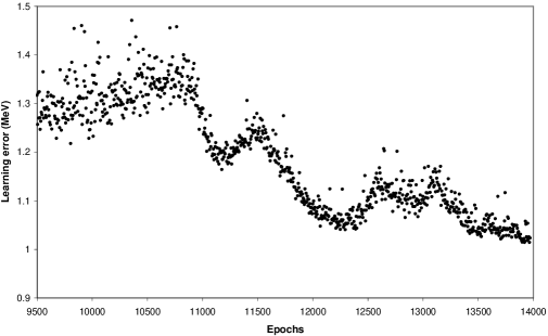
Figure 1: Time course of the learning error ($\sigma_{\mathrm{r}ms}$) for a network trained with the modified backpropagation (MB) algorithm defined by eqs. (3) and (4) (typical example).

In training neural networks, there is always the question of when to stop the process. If the network is trained for too short a period, the training data will not be adequately fitted. On the other hand, if the training period is continued for too long, generalization (i.e. prediction) will suffer, since the “overtrained” network will be specialized to the idiosyncrasies of the particular learning set that has been supplied. Thus some reasonable compromise must be struck between the desiderata of a good fit and good prediction. In our computer experiments, we have adopted the following criterion. A given training run consists of a relatively large number of epochs, specified beforehand. During such a run, we monitor not only the cost function for the patterns in the learning set, but also for a separate validation set of nuclei whose masses are known. The “trained” network model resulting from a given run is taken as that network with the set of connection weights producing the smallest value of the cost function on the validation set, over the full course of the run. While the members of the validation set are not used in the weight updates of the MB (or SB) training rule, they clearly do affect the choice of model. Therefore, accuracy on the validation set cannot strictly be regarded as a measure of predictive performance, although in practice it may still provide a useful indicator of this aspect of the model. To obtain a clean measure of predictive performance, still a third set of examples is needed: a test (prediction) set that is never referred to during the training process.

Another general problem that one faces in training neural networks is that of the optimal architecture in terms of the numbers of layers and the numbers of units in each layer. As in most neural-network applications, we have simply followed a “trial-and-error” approach to this problem; certainly no claim can be made that a full optimization has been achieved.

Numerical experiments have shown that performance can be improved by modifying the learning rate $\eta$ and momentum parameter $\alpha$ during training. In applying the MB algorithm, $\eta$ and $\alpha$ are assigned starting values 0.5 and 0.9, respectively, and the validation error is calculated every five epochs. If this error decreases for two or more consecutive evaluations, the learning rate $\eta$ (with $0<\eta<3)$ is increased by 0.02; otherwise it is decreased by 0.005. The momentum parameter $\alpha$ is usually set to $0.9999$ when $e$ becomes relatively large. Comparative studies of the mass-modeling problem (to be summarized in Table 1 of Section 3) demonstrate that this training procedure, in conjunction with the MB update rule (3)–(4), generally yields better results than does the SB algorithm.

The evolution of the learning error under application of the MB algorithm is illustrated by the sample shown in fig. 1. We emphasize that this algorithm departs from gradient descent, allowing the network to escape from local minima.

2.3 Data Sets

In exploring the prospects for statistical modeling of nuclear mass excesses, we have primarily employed a database O+N made up of (i) $1323$ “old” (O) experimental masses which the 1981 Möller-Nix theoretical model [8] was designed to reproduce, together with (ii) $351$ “new” (N) experimental masses, measured subsequently for nuclei that lie mostly beyond the edges of the 1981 data collection when viewed in the $N-Z$ plane. As discussed in ref. [1], the O and N data sets were selected as part of a strategy for quantifying the extrapolation capability (“extrapability”) of global mass models – i.e., their ability to predict the atomic masses for nuclides far from stability. These sets have also been used in evaluating the predictive performance of neural network models of the atomic mass function, with set O providing the fitting data (learning set) and set N the target data for prediction (test set) (e.g., see ref. [21]).

To further characterize the interpolation/extrapolation capability of our models, we have also employed two data sets of $1303$ (M1) and $351$ (M2) nuclei and their masses, chosen randomly from the union of the O and N sets, after excluding 20 nuclides with poorly measured masses. Together, these $1654$ cases form the database fitted by the FRDM parametrization of ref. [10], i.e., by the best of the mid-90’s theoretical models developed by the Los Alamos-Berkeley Group. We also make use of another set of $158$ nuclei (denoted NB) that lie outside the O and N databases, the experimental masses of these examples being drawn from the NUBASE evaluation of nuclear and decay properties [3]. The locations of the nuclei of the O, N, and, NB sets in the $N-Z$ plane are shown in fig. 2.

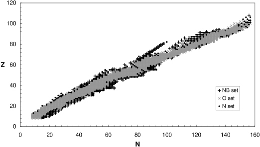
Figure 2: Locations in the $N-Z$ plane are indicated for the O, N, and, NB data sets employed in neural-network modeling of nuclear mass excesses (see section 2.3).

2.4 Coding at Input and Output Interfaces

We have considered several input coding schemes designed to facilitate learning of quantal properties (pairing, shell structure) that depend on the integral nature of $Z$ and $N$ (see refs. [20, 21, 26]). The scheme that achieves this aim most efficiently while keeping the number of weights to a minimum is one that implements analog (floating-point) coding of $Z$ and $N$ in terms of the inputs of only two dedicated analog input neurons, which, however, are aided by two further binary (“on-off”) input units that encode the parity (even or odd) of $Z$ and $N$ [26]. The analog input units scale the $Z$ and $N$ values to the interval [0,1] in such a manner that the stimuli received by the logistic units in hidden and output layers remain within their best dynamical range. A less efficient scheme, introduced in ref. [20], utilizes banks of on-off units to represent $Z$ and $N$ as binary integers.

The mass excess computed by the network is represented by the activity of a single analog output unit. For the same reason as for the input units representing $Z$ and $N$, the target mass excess values $\Delta M$ are also scaled to the interval [0,1].

Several prescriptions have been tried for scaling the $Z$, $N$, and $\Delta M$ variables, two of which are represented in the results reported here. Extensive comparative studies of the MB and SB training algorithms were based on the P1 prescription, which admits the ranges $[0,110]$, $[0,160]$, and $[-110,130]$ for the variables $Z$, $N$, and $\Delta M$, respectively. In later work we adopted the P2 prescription, which allows for the extended respective ranges $[0,130]$, $[0,200]$, and $[-110,250]$, thereby providing ample room for new nuclei far from the stable valley. The latter scaling recipe usually gives better results.

3 Results

We first present results of a comparative study of the quality of models generated with the modified back-propagation training algorithm MB and with the standard back-propagation routine SB. Seven pairs of models were constructed, one member of each pair being trained with MB and the other with SB, and both members of the pair being started from the same choice among seven different sets of random initial weights. All of these models have architecture ($4$–$10$–$10$–$10$–$1$)[281] and employ the P1 scaling recipe. In all seven cases, the values of the error measures $\sigma_{\mathrm{r}ms}$ attained by the MB algorithm for the learning, validation, and test sets are consistently smaller than the corresponding values achieved with SB. A similar pattern is expected to hold for the P2 scaling prescription.

Table 1: Performance comparison of standard back-propagation (SB) and modified back-propagation (MB) training algorithms in the task of mass modeling. Results for the rms error $\sigma_{\mathrm{r}ms}$ on learning, validation, and test sets are given for seven pairs of models with network architecture ($4$–$10$–$10$–$10$–$1$)[281]. The members of each model pair belong to the same choice among seven initial sets of random weights. All models have been trained for a total of 20,000 epochs using the P1 scaling recipe defined in Section 2.4.

Set	Algorithm	learning (O) set $\sigma_{\mathrm{r}ms}$(MeV)	validation (N) set $\sigma_{\mathrm{r}ms}$(MeV)	test (NB) set $\sigma_{\mathrm{r}ms}$(MeV)
1	MB	0.78	1.92	2.84
	SB	1.27	2.57	3.12
2	MB	0.78	1.93	2.34
	SB	1.11	3.73	4.53
3	MB	0.71	1.25	1.88
	SB	0.92	1.58	2.44
4	MB	0.98	1.81	3.10
	SB	1.31	3.88	4.36
5	MB	0.69	1.54	2.14
	SB	1.32	2.06	2.79
6	MB	0.66	1.65	2.73
	SB	0.96	1.81	3.03
7	MB	0.62	1.59	2.01
	SB	0.98	3.71	3.97

Specializing to the MB algorithm, we have carried out a substantial number of computer experiments for networks with various architectures and for networks with the same architecture but different random choices of initial weights.

Performance measures of some of our best models (marked with asterisks) are reported in Table 2, together with similar performance data for two neural-network models from earlier studies and for three high-quality theoretical models, two from Möller et al. [1, 10] and one due to Pearson et al. [13]. The table entries are separated into two groups by a pair of horizontal lines.

Table 2: Performance measures of global models of the atomic mass table derived from neural-network technology and from conventional theory and phenomenology (see text for details). Data sets are indicated in parentheses. Those rms error measures referring to actual predictions, rather than fits, are printed in italic font.

Network architecture ($I$–$H_{1}$–$H_{2}$–…–$H_{L}$–$O$)[$P$]	learning set $\sigma_{\mathrm{r}ms}$(MeV)	validation set $\sigma_{\mathrm{r}ms}$(MeV)	test set $\sigma_{\mathrm{r}ms}$(MeV)
Möller et al. (ref. [1])	0.67 (O)	–	0.74 (N)
($18$–$10$–$10$–$10$–$1$)[421] (ref. [21]) $Z$ & $N$ in binary $A$ & $Z-N$ in analog	0.83 (O)	–	5.98 (N)
($4$–$40$–$1$)[245] (ref. [30])	1.07 (O)	–	3.04 (N)
($4$–$10$–$10$–$10$–$1$)∗[281] $Z$ & $N$ in analog and parity	0.71 (O)	2.28 (NB)	2.16 (N)
Support Vector Machine (ref. [31])	0.70 (O)	–	0.75 (N)
Möller et al. (ref. [10])	0.68 (M1)	0.71 (M2)	0.70 (NB)
Pearson et al. (ref. [13])	0.67 (M1)	0.68 (M2)	0.73 (NB)
($4$–$10$–$10$–$10$–$1$)∗∗[281] $Z$ & $N$ in analog and parity	0.41 (M1)	0.47 (M2)	1.48 (NB)
($4$–$10$–$10$–$10$–$1$)∗∗∗[361] $Z$ & $N$ in analog and parity	0.44 (M1)	0.44 (M2)	0.95 (NB)

The generalization ability (extrapability) of models belonging to the first group, whether statistical or theoretical, was assessed by treating the N data set as a test set. In this way, results obtained by the neural-network approach could be directly compared with the results [1] of the extrapability study carried out by the Los Alamos-Berkeley group for the FRDM approach (and especially with the rms error values shown in the first row of Table 2). The first of the network models selected from earlier studies is of the five-layer architecture ($18$–$10$–$10$–$10$–$1$)[421]; it was constructed by Gernoth et al. [21] using standard back-propagation, with binary encoding of $Z$ and $N$ and “redundant” analog encoding of the atomic mass number $A$ and the neutron excess $N-Z$. The three-layer network ($4$–$40$–$1$)[245] is due to Kalman, who adopted analog coding of $Z$ and $N$ and auxiliary parity units for these variables. In training this model, the input patterns were pre-processed by singular-value decomposition and the cost function minimized by a Powell-update conjugate-gradient algorithm (for additional details, see refs. [23, 30]).

The network model labeled with one asterisk was one of those created mainly for evaluating the modified training procedure MB. It has the five-layer architecture ($4$–$10$–$10$–$10$–$1$)[281] and employs parity-aided input coding and the scaling recipe P1. Utilization of the NB data for validation gives this model an a priori advantage over the earlier network models, for which only the learning set was involved in the training process. This advantage is clearly realized in practice.

Also included in the first group is a set of results [31] obtained recently with a Support Vector Machine [32, 33].

The network models appearing in the second group employ the scaling recipe P2 and were trained with the mixed data sets M1 and M2 described in section 2.3. Thus, the training and validation examples include, in this case, members from both the O and N data sets. The intent was to develop statistical models that can be compared more directly with the most refined FRDM model of ref. [10], recalling that the parameters of this model were fit to the 1654 examples of the M1+M2 database. The network model marked with two asterisks has the same five-layer architecture and number of weight parameters as the (*) network. In the network model marked with three asterisks, we chose to introduce connections from the analog input units to all units of all the hidden layers, to avoid or reduce the degradation of information as it propagates toward the output unit. However, this innovation comes at the expense of increasing the number of weight parameters from the $281$ of the (**) network to $361$. The resulting system is the best neural-network model of the mass table yet achieved, based on the accuracy of the estimated masses of the NB set of nuclides, taken as the test set. The corresponding rms error is 0.95 MeV, which is to be compared with the figure 0.70 MeV obtained in the FRDM evaluation. Also included in the third group are the corresponding rms errors for the HFB2 model [13]. The parameters of this model have been adjusted to an extended data set of $1888$ nuclei, which however includes the $158$ nuclei of the NB set.

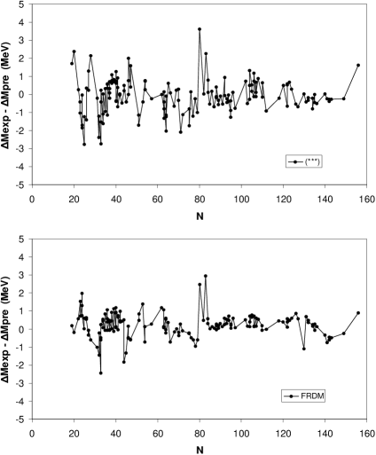
Figure 3: Top panel: Deviations from experiment (in MeV) of mass-excesses values predicted by the neural-network model ($4$–$10$–$10$–$10$–$1$)^∗∗∗ for the NUBASE (NB) nuclei identified in fig. 2. The plot represents a projection of the mass surface onto a plane of constant $Z$ and thus shows dependence on neutron number $N$. Bottom panel: Same for the FRDM evaluation [10].

Further information on the performance of the (***) network is furnished in fig. 3. Here we compare the deviations from experimental data of the mass-excess values generated by the net and by the FRDM evaluation, for the NB nuclei. The extrapolation capability of the (***) network model is better illustrated in fig. 4, which shows these deviations as a function of the number of neutrons away from the $\beta^{-}$ stability line.

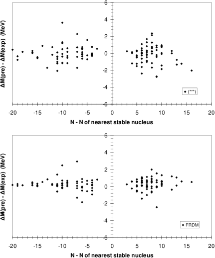
Figure 4: Top panel: Deviations from experiment (in MeV) of mass-excesses values predicted by the neural-network model ($4$–$10$–$10$–$10$–$1$)^∗∗∗ for the NUBASE (NB) nuclei identified in fig. 2, as a function of the number of neutrons away from the line of $\beta^{-}$ stability. Bottom panel: Same for the FRDM evaluation [10].

In spite of its residual shortcomings, the current generation of neural-network models of the mass table represents a significant step toward extrapability levels comparable with those reached by the best traditional global models rooted in quantum theory. The ultimate test of any class of global mass models is the accuracy that can be realized in the prediction of masses of nuclear species prior to measurement. A text data file containing the mass-excess values predicted by the (***) network for 7709 nuclides ($Z,N\geq 8$, $Z<120$, $N<200$) is available for downloading from http://www.cc.uoa.gr/$\sim$sathanas/mass_excess (see file “massfiles.txt” for details).

4 Conclusions and prospects

The present investigation is a continuation and an elaboration of a research thrust [20, 21, 22, 23, 24, 25] that seeks to develop accurate global models of nuclear properties with demonstrable predictive power, within the arena of statistical methods based on multilayer neural networks. Our particular concern has been the central problem of modeling the systematics of nuclear mass excesses. We have introduced a modified back-propagation algorithm (MB) along with new prescriptions for encoding and decoding input and output patterns. The study has been based mainly on data sets selected by Möller and Nix [1] for the purpose of testing the extrapolation capabilities of global models of atomic masses. As seen in Table 2, our best network models of the nuclear mass excess $\Delta M$ display substantially improved performance relative to earlier attempts that use neural networks to predict masses far from the valley of $\beta$ stability. A strong impetus for further improvement of this approach comes from the production of new nuclei at radioactive beam facilities and heavy-ion colliders, as well as by the needs of supernova modeling and state-of-the-art theories of nucleosynthesis.

In closing, we would like to emphasize the conceptual and structural differences between

• statistical models of the atomic-mass function constructed with the aid of learning rules operating purely on the experimental data, without any overt imposition of physical principles and theory, and

• the familiar theory-based phenomenological models, constrained by the data.

Although the latter models become more elaborate as the standards of description increase, they are nevertheless relatively compact, having relatively few adjustable parameters, with transparent physical meaning. By contrast, the neural-network methodology is a more abstract kind of “engine” that generates a statistical representation of the experimental data having many parameters. While this representation may have strong predictive power, its parameters are ordinarily (though not always) opaque to physical interpretation. In view of these fundamental differences, the two approaches should more fruitfully be viewed as complementary, rather than in competition.

We are currently exploring and implementing a number of refinements of neural-network approaches to the mass problem. These include the introduction of diverse pruning and network construction schemes and the application of other more powerful training (optimization) procedures. Additionally, we have made some initial attempts to construct an informative statistical model of the differences between the experimental mass-excess values $\Delta M^{\rm exp}$ and the theoretical values $\Delta M^{\rm th}$ given by the FRDM model of Möller et al. [10]. This study is being pursued with the hope of revealing subtle regularities of nuclear structure not yet embodied in the best microscopic/phenomenological models of atomic-mass systematics. To date, the results have not been illuminating in terms of the emergence of systematic trends – a tentative finding which, if sustained, could imply that the residual physical corrections to the theoretical model are small but numerous, and of fluctuating size and sign. Also under investigation is the potential of Support Vector Machines [32, 33] for systematic development of near-optimal statistical models of atomic masses and other nuclear properties. The results reported in table 2 are suggestive of the power of this approach.

5 Addendum

After completing the training of the (***) network, the AME$03$ atomic mass evaluation [34] was published. This compilation made available precision mass measurements for nuclei farther off the stability line, while providing corrected mass-excess values for nuclei already used in our study. The next generation of neural-network models will be trained using the AME$03$ data. Already, however, we can further appraise the extrapability performance of the (***) network, the best neural-network model of the mass table yet achieved, by making use of $529$ new nuclei included in the AME$03$ evaluation, which extend beyond the edges of the $1654$-nuclide set M1+M2 as viewed in the $N-Z$ plane. A text data file containing the predicted mass-excess values for these $529$ additional nuclides is available for downloading from http://www.cc.uoa.gr/$\sim$sathanas/ mass_excess (see file “massfiles.txt” for details). The resulting value of $\sigma_{\mathrm{r}ms}$ for these nuclei is 1.03 MeV, which is to be compared with the figures 0.58 MeV and 0.67 MeV obtained in the FRDM and HFB2 evaluations. When comparing these results, it should be kept in mind that the parameters of the HBF2 model have been adjusted by making use of an extended data set of $1888$ nuclei, which includes $255$ of the $529$ nuclides.

References

- [1] P. Möller and J. R. Nix, J. Phys. G 20 (1994) 1681.
- [2] C. Borcea and G. Audi, Rom. J. Phys. 38 (1993) 455.
- [3] G. Audi, O. Bersillon, J. Blachot, and A. H. Wapstra, Nucl. Phys. A624 (1997) 1.
- [4] M. Uno, Riken Review 26 (2000) 38.
- [5] J. M. Pearson, Hyperfine Interactions 132 (2001) 59.
- [6] D. Lunney, J. M. Pearson and , C. Thibault, Rev. Mod. Phys. 75 (2003) 1021.
- [7] Opportunities in Nuclear Science: “A Long Range Plan in the Next Decade” (DOE/NSF, 2002) ; “Nuclear Physics in Europe: Highlights and Opportunities” (NUPECC, 1997).
- [8] P. Möller and J. R. Nix, At. Data Nucl. Data Tables 26 (1981) 165.
- [9] P. Möller and J. R. Nix, At. Data Nucl. Data Tables 39 (1988) 213 ; P. Möller, W. D. Myers, W. J. Swiatecki, and J. Treiner, ibid. 39 (1988) 225.
- [10] P. Möller, J. R. Nix, W. D. Myers, and W. J. Swiatecki, At. Data Nucl. Data Tables 59 (1995) 185.
- [11] Y. Aboussir, J. M. Pearson, A. K. Dutta and F. Tondeur, At. Data Nucl. Data Tables 61 (1995) 127.
- [12] S. Goriely, F. Tondeur and J. M. Pearson, At. Data Nucl. Data Tables 77 (2001) 311.
- [13] (a) M. Samyn, S. Goriely, P.-H. Heenen, J. M. Pearson and F. Tondeur, Nucl. Phys. A700 (2002) 142 ; (b) S. Goriely, M. Samyn, P.-H. Heenen, J. M. Pearson and F. Tondeur, Phys. Rev. C66 (2002) 024326.
- [14] V. Cherkassky, J. H. Friedman, and W. Wechsler, eds., From Statistics to Neural Networks. Theory and Pattern Recognition Applications (Springer-Verlag, Berlin, 1994).
- [15] J. W. Clark, T. Lindenau, and M. L. Ristig, eds., Scientific Applications of Neural Nets (Springer-Verlag, Berlin, 1999).
- [16] J. Hertz, A. Krogh, and R. G. Palmer, Introduction to the Theory of Neural Computation (Addison-Wesley, Redwood City, CA, 1991).
- [17] J. W. Clark, Phys. Med. Biol. 36 (1992) 1259.
- [18] S. Haykin, Neural Networks: A Comprehensive Foundation (McMillan, New York, 1998).
- [19] C. Bishop, Neural Networks for Pattern Recognition (Clarendon, Oxford, 1995).
- [20] S. Gazula, J. W. Clark, and H. Bohr, Nucl. Phys. A540 (1992) 1.
- [21] K. A. Gernoth, J. W. Clark, J. S. Prater, and H. Bohr, Phys. Lett. B300 (1993) 1.
- [22] K. A. Gernoth and J. W. Clark, Neural Networks 8 (1995) 291.
- [23] K. A. Gernoth and J. W. Clark, Comp. Phys. Commun. 88 (1995) 1.
- [24] J. W. Clark, in Scientific Applications of Neural Nets, J. W. Clark, T. Lindenau, and M. L. Ristig, eds. (Springer-Verlag, Berlin, 1999), p. 1.
- [25] K. A. Gernoth, in Scientific Applications of Neural Nets, J. W. Clark, T. Lindenau, and M. L. Ristig, eds. (Springer-Verlag, Berlin, 1999), p. 139.
- [26] S. Athanassopoulos, MSc thesis, University of Athens, 1998.
- [27] E. Mavrommatis, A. Dakos, K. A. Gernoth, and J. W. Clark, Condensed Matter Theories, Vol. 13, J. da Providencia and F. B. Malik, eds. (Nova Science Publishers, Commack, NY, 1998) p. 423
- [28] E. Mavrommatis, S. Athanassopoulos, K. A. Gernoth, and J. W. Clark, Condensed Matter Theories, Vol. 15, G. S. Anagnostatos et al., eds. (Nova Science Publishers, Commack, N.Y., 2000) p. 207
- [29] J. W. Clark, E. Mavrommatis, S. Athanassopoulos, A. Dakos and K. A. Gernoth in Proceedings of the Conference on “Fission Dynamics of Atomic Clusters and Nuclei”, D. M. Brink et al., eds. (World Scientific, Singapore) pp. 76-85
- [30] B. L. Kalman, private communication.
- [31] H. Li, J. W. Clark, S. Athanassopoulos, E. Mavrommatis, and K. A. Gernoth, to be published.
- [32] V. Vapnik, The Nature of Statistical Learning Theory (Springer-Verlag, Heidelberg, 1995).
- [33] N. Cristianini and John Shawe-Taylor, An Introduction to Support Vector Machines and Other Kernel-based Learning Methods (Cambridge University Press, Cambridge, 2002).
- [34] A. H. Wapstra, G. Audi, and C. Thibault, Nucl. Phys. A729 (2003) 337.