How to derive and compute 1,648 diagrams

Abstract

We present the first calculation for many-electron atoms complete through fourth order of many-body perturbation theory. Owing to an overwhelmingly large number of underlying diagrams, we developed a suite of symbolic algebra tools to automate derivation and coding. We augment all-order single-double excitation method with 1,648 omitted fourth-order diagrams and compute amplitudes of principal transitions in Na. The resulting ab initio relativistic electric-dipole amplitudes are in an excellent agreement with 0.05%-accurate experimental values. Analysis of previously unmanageable classes of diagrams provides a useful guide to a design of even more accurate, yet practical many-body methods.

Many-body perturbation theory (MBPT) has proven to be a powerful tool in physics Fetter and Walecka (1971) and quantum chemistry Szabo and Ostlund (1982). Although MBPT provides a systematic approach to solving many-body quantum-mechanical problem, the number and complexity of analytical expressions and thus challenges of implementation grow rapidly with increasing order of MBPT (see Fig.1) Indeed, because of this complexity it has proven to be difficult to go beyond the complete third order in calculations for many-electron atoms (see, e.g., review Sapirstein (1998)). At the same time, studies of higher orders are desirable for improving accuracy of ab initio atomic-structure methods. Such an improved accuracy is required, for example, in interpretation of atomic parity violation PNC and unfolding cosmological evolution of the fine-structure constant $\alpha$ Webb et al. (2001).

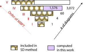
Figure 1: Number of diagrams grows rapidly with the order of MBPT. Here we show number of topologically distinct Brueckner-Goldstone diagrams for transition amplitudes for univalent atoms. We assume that calculations are carried out in $V^{N-1}$ Hartree-Fock basis to minimize the number of diagrams and we do not count “folded” Lindgren and Morrison (1986) and normalization diagrams. All-order single-double (SD) excitations method recovers all diagrams through the third order, but misses roughly a half of diagrams in the fourth order. These 1,576 missed diagrams and 72 related normalization diagrams are explicitly computed in the present work.

Here we report the first calculation of transition amplitudes for alkali-metal atoms complete through the fourth order of MBPT. We explicitly computed 1,648 topologically distinct Brueckner-Goldstone diagrams. To overcome such an overwhelming complexity we developed a symbolic problem-solving environment that automates highly repetitive but error-prone derivation and coding of many-body diagrams. Our work illuminates a crucial role of symbolic tools in problems unsurmountable in the traditional “pencil-and-paper” approach. Indeed, third-order calculation Blundell et al. (1987); Johnson et al. (1996) was a major research project most likely to have required a year to accomplish. As one progresses from the third to the present fourth order (see Fig. 1) there is a 50-fold increase in the number of diagrams. Simple scaling shows that present calculations require half a century to complete. With our tools derivation and coding take just a few minutes. Similar symbolic tools were developed by Perger et al. (2001), however their package is so far limited to well-studiedBlundell et al. (1990a); Johnson et al. (1996) third order of MBPT. In contrast, we explore a wide range of new, previously unmanageable, classes of diagrams.

As an example of application of our symbolic technology, we compute electric-dipole amplitudes of the principal $3p_{3/2}-3s_{1/2}$ and $3p_{1/2}-3s_{1/2}$ transitions in Na. We augment all-order single-double excitations method Safronova et al. (1998) with 1,648 diagrams so that the formalism is complete through the fourth order ( see Fig.1 ). The results are in excellent agreement with 0.05%-accurate experimental values Jones et al. (1996). Thus our computational method not only enables exploration of a wide range of previously unmanageable classes of diagrams but also defines new level of accuracy in ab initio relativistic atomic many-body calculations. Atomic units $|e|=\hbar=m_{e}=4\pi\varepsilon_{0}\equiv 1$ are used throughout this paper.

Method— A practitioner of atomic MBPT typically follows these steps: (i) derivation of diagrams, (ii) angular reduction, and (iii) coding and numerical evaluation. Below we highlight components of our problem-solving environment designed to assist a theorist in these technically-involved tasks. First we briefly reiterate MBPT formalism Derevianko and Emmons (2002) for atoms with a single valence electron outside a closed-shell core. For these systems a convenient point of departure is a single-particle basis generated in frozen-core ($V^{N-1}$) Dirac-Hartree-Fock (DHF) approximation Kelly (1969). In this approximation the number of MBPT diagrams is substantially reduced Lindgren and Morrison (1986); Blundell et al. (1987). The lowest-order valence wavefunction $|\Psi_{v}^{(0)}\rangle$ is simply a Slater determinant constructed from core orbitals and proper valence state $v$. The perturbation expansion is built in powers of residual interaction $V_{I}$ defined as a difference between the full Coulomb interaction between the electrons and the DHF potential. The $n^{\mathrm{th}}$-order correction to the valence wavefunction may be expressed as

$$|\Psi_{v}^{(n)}\rangle=-R_{v}\left\{Q\,V_{I}\,|\Psi_{v}^{(n-1)}\rangle\right\}_{\mathrm{linked}}\,,$$ (1)

where $R_{v}$ is a resolvent operator modified to include so-called “folded” diagrams Derevianko and Emmons (2002), projection operator $Q=1-|\Psi_{v}^{(0)}\rangle\langle\Psi_{v}^{(0)}|$, and only linked diagrams Lindgren and Morrison (1986) are to be kept. From this recursion relation we may generate corrections to wave functions at any given order of perturbation theory. With such calculated corrections to wavefunctions of two valence states $w$ and $v$, $n^{\mathrm{th}}$-order contributions to matrix elements of an operator $\hat{Z}$ are

$$Z^{(n)}_{wv}=\sum_{k=0}^{n-1}\langle\Psi_{w}^{(n-k-1)}|Z|\Psi_{v}^{(k)}\rangle_{\mathrm{val,\,conn}}+Z^{(n)}_{wv,\,{\rm norm}}\,.$$ (2)

Here $Z^{(n)}_{wv,\,{\rm norm}}$ is a normalization correction arising due to an intermediate normalization scheme employed in derivation of Eq. (1). Subscript “$\mathrm{val,\,conn}$” indicates that only connected diagrams involving excitations from valence orbitals are included in the expansion.

Equations (1) and (2) completely define a set of many-body diagrams at any given order of MBPT. In practice the derivations are carried out in the second quantization and the Wick’s theorem Lindgren and Morrison (1986) is used to simplify products of creation and annihilation operators. Although the application of the Wick’s theorem is straightforward, as order of MBPT increases, the sheer length of expressions and number of operations becomes quickly unmanageable. We developed a symbolic-algebra package written in Mathematica Wolfram (1999) to carry out this task. The employed algorithm relies on decision trees and pattern matching, i.e., programming elements typical to artificial intelligence applications. With the developed package we fully derived fourth-order corrections to matrix elements of univalent systems Derevianko and Emmons (2002).

This is one of the fourth-order terms from Ref. Derevianko and Emmons (2002)

$$\sum_{abc}\sum_{mnr}\frac{{z_{bv}}{\tilde{g}}_{canr}{g_{nrcm}}{\tilde{g}}_{mwab}}{({{\varepsilon}_{w}}-{{\varepsilon}_{b}})\,({{\varepsilon}_{mw}}-{{\varepsilon}_{ab}})\,({{\varepsilon}_{nrw}}-{{\varepsilon}_{abc}})}\,\,.$$ (3)

There are 524 such contributions in the fourth order nmb . Here abbreviation $\varepsilon_{xy\ldots z}$ stands for $\varepsilon_{x}+\varepsilon_{y}+\cdots\varepsilon_{z}$, with $\varepsilon_{x}$ being single-particle DHF energies. Further, $g_{ijlk}$ are matrix elements of electron-electron interaction in the basis of DHF orbitals. The quantities $\tilde{g}_{ijlk}$ are antisymmetric combinations $\tilde{g}_{ijlk}={g}_{ijlk}-{g}_{ijkl}$. The summation is over single-particle DHF states. Core orbitals are enumerated by letters $a,b,c$ and complementary excited states are labelled by $m,n,r$. Finally matrix elements of the operator $\hat{Z}$ in the DHF basis are denoted as $z_{ij}$.

The summations over magnetic quantum numbers are usually carried out analytically. This “angular reduction” is the next major technically-involved step. We also automate this task. The details are provided in Ref. Derevianko . Briefly, the angular reduction is based on application of the Wigner-Eckart (WE) theorem Edmonds (1985) to matrix elements $z_{ij}$ and $g_{ijkl}$. The WE theorem allows one to “peel off” dependence of the matrix elements on magnetic quantum numbers in the form of 3j-symbols and reduced matrix elements. In the particular case of fourth-order terms, such as Eq. (3), application of the WE theorem results in a product of seven 3j-symbols. To automate simplification of the products of 3j-symbols we employed a symbolic program Kentaro developed by Takada (1992).

The result of angular reduction of our sample term (3) is

$$\sum_{abcmnr}\sum_{L}\frac{\delta_{j_{a}j_{m}}\,\delta_{j_{b}j_{w}}\,{\left(-1\right)}^{j_{a}+j_{c}+j_{n}+j_{r}}\,}{(2L+1)\,{\sqrt{(2j_{a}+1)(2j_{w}+1)}}}$$

$$\frac{\langle b||z||v\rangle\,Z_{L}(canr)X_{L}(nrcm)\,Z_{0}(mwab)\,}{({{\varepsilon}_{w}}-{{\varepsilon}_{b}})\,({{\varepsilon}_{mw}}-{{\varepsilon}_{ab}})\,({{\varepsilon}_{nrw}}-{{\varepsilon}_{abc}})}\,.$$

Here the reduced quantities $\langle i||z||j\rangle$, $X_{L}(ijkl)$, and $Z_{L}(ijkl)$ depend only on total angular momenta and principal quantum numbers of single-particle orbitals.

As a result of angular reduction we generate analytical expressions suitable for coding. We also automated the tedious coding process by developing custom parsers based on Perl and Mathematica. These parsers translate analytical expressions into Fortran90 code. The resulting code is very large - it is about 20,000 lines long and were it be programmed manually, it would have required several years to develop. For numerical evaluation we employed a B-spline libraryJohnson et al. (1988). All the fourth-order results were computed with a sufficiently large basis of 25 out of 30 lowest-energy ($E>mc^{2}$) spline functions for each partial wave through $h_{11/2}$.

At this point we have demonstrated feasibility of working with thousands of diagrams in atomic MBPT. Now we apply our computational technique to high-accuracy calculation of transition amplitudes in Na.

Fourth-order diagrams complementary to single-double excitations method. One of the mainstays of practical applications of MBPT is an assumption of convergence of series in powers of the perturbing interaction. Sometimes the convergence is poor and then one sums certain classes of diagrams to “all orders” using iterative techniques. In fact, the most accurate many-body calculations of parity violation in Cs by Dzuba et al. (1989) and Blundell et al. (1990b) are of this kind. These techniques, although summing certain classes of MBPT diagrams to all orders, still do not account for an infinite number of residual diagrams (see Fig. 1). In Ref. Derevianko and Emmons (2002) we proposed to augment a given all-order technique with some of the omitted diagrams so that the formalism is complete through a certain order of MBPT. As in that work, here we consider an improvement of all-order single-double (SD) excitation method employed in Ref. Blundell et al. (1990b). Here a certain level $n$ of excitations from lowest-order wavefunction refers to an all-order grouping of contributions in which $n$ core and valence electrons are promoted to excited single-particle orbitals. The SD method is a simplified version of the coupled-cluster expansion truncated at single and double excitations.

The next step in improving the SD method would be an inclusion of triple excitations. However, considering present state of available computational power, the complete incorporation of triples seems as yet impractical for heavy atoms. Here we investigate an alternative illustrated in Fig. 1 : we compute the dominant contribution of triples in a direct fourth-order MBPT for transition amplitudes. We also account for contribution of disconnected quadruple excitations in the fourth order. In Ref. Derevianko and Emmons (2002), we separated these complementary diagrams into three major categories by noting that triples and disconnected quadruples enter the fourth order matrix element $Z^{(4)}_{wv}$ via (i) an indirect effect of triples and disconnected quadruples on single and double excitations in the third-order wavefunction — we denote this class as $Z_{0\times 3}$; (ii) direct contribution to matrix elements labelled as $Z_{1\times 2}$; (iii) correction to normalization denoted as $Z_{\mathrm{norm}}$. Further these categories were broken into subclasses based on the nature of triples, so that

$$\left(Z^{(4)}_{wv}\right)_{\mathrm{non-SD}}=Z_{1\times 2}(T_{v})+Z_{1\times 2}(T_{c})+$$

$$Z_{0\times 3}(S_{v}[T_{v}])+Z_{0\times 3}(D_{v}[T_{v}])+$$

$$Z_{0\times 3}(S_{c}[T_{c}])+Z_{0\times 3}(D_{v}[T_{c}])+$$

$$Z_{1\times 2}\left(D_{\mathrm{n}l}\right)+Z_{0\times 3}\left(D_{\mathrm{n}l}\right)+Z_{\mathrm{norm}}(T_{v})\,.$$

Here we distinguished between valence ($T_{v}$) and core ($T_{c}$) triples and introduced a similar notation for singles ($S$) and doubles ($D$). Notation like $S_{v}[T_{c}]$ stands for effect of second-order core triples ($T_{c}$) on third-order valence singles $S_{v}$. Diagrams $D_{\mathrm{nl}}$ are contributions of disconnected quadruples (non-linear contributions from double excitations). The reader is referred to Ref. Derevianko and Emmons (2002) for further details and discussion.

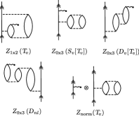
Figure 2: Representative fourth-order diagrams involving triple and disconnected quadruple excitations.

Transition amplitudes in Na. Using our problem-solving environment we derived the 1,648 complementary diagrams Derevianko and Emmons (2002), carried out angular reduction Derevianko , and generated Fortran 90 code suitable for any univalent system. As an example we evaluate reduced electric-dipole matrix elements of $3s_{1/2}-3p_{1/2,3/2}$ transitions in Na (eleven electrons)com (a). Our numerical results are presented in Table 1. Analyzing this table we see that leading contributions come from valence triples $T_{v}$. Similar conclusion can be drawn from our preliminary calculations for heavier Cs atom. Dominance of valence triples ($T_{v}$) over core triples ($T_{c}$) may be explained by smaller energy denominators for $T_{v}$ terms. Representative diagrams for these relatively large contributions are shown in Fig. 2. Based on this observation we propose to fully incorporate valence triples into a hierarchy of coupled-cluster equations and add a perturbative contributions of core triples. Such an all-order scheme would be a more accurate and yet practical extension of the present calculations.

Another point we would like to discuss is a sensitivity of our results to higher-order corrections. In Table 1, all large contributions add up coherently, possibly indicating a good convergence pattern of MBPT. However, we found large, factor of 100, cancellations of terms inside the $Z_{0\times 3}(S_{v}[T_{v}])$ class. In principle higher-order MBPT corrections may offset a balance between cancelling terms and an all-order treatment is desired. Fortunately, the $Z_{0\times 3}(S_{v}[T_{v}])$ class of diagrams (combined with parts of $Z_{1\times 2}(T_{v})$) have been taken into account in all-order SDpT (SD + partial triples) method Blundell et al. (1990b); Safronova et al. (1999). We correct our results for the difference between all-order com (b) and our fourth-order values for these diagrams (last row of Table 1). These all-order corrections modify our final values of complementary diagrams by 15%.

Class	Number of	$3p_{1/2}-3s_{1/2}$	$3p_{3/2}-3s_{1/2}$
	diagrams
Connected triples
$Z_{0\times 3}(S_{v}[T_{v}])$	72	$-0.8[-3]$	$-1.1[-3]$
$Z_{0\times 3}(D_{v}[T_{v}])$	432	$-2.2[-3]$	$-3.0[-3]$
$Z_{1\times 2}(T_{v})$	504	$-0.7[-3]$	$-1.0[-3]$
$Z_{\mathrm{norm}}(T_{v})$	72	$-0.7[-3]$	$-1.2[-3]$
$Z_{0\times 3}(D_{v}[T_{c}])$	144	$-0.01[-3]$	$-0.01[-3]$
$Z_{0\times 3}(S_{c}[T_{c}])$	72	$0.06[-3]$	$0.09[-3]$
$Z_{1\times 2}(T_{c})$	216	$0.03[-3]$	$0.04[-3]$
Total triples	1512	$-4.3[-3]$	$-6.3[-3]$
Disconnected quadruples
$Z_{0\times 3}(D_{nl})$	68	$1.1[-3]$	$1.6[-3]$
$Z_{1\times 2}(D_{nl})$	68	$0.2[-3]$	$0.3[-3]$
Total quads	136	$1.4[-3]$	$2.0[-3]$
Total	1648	$-2.6[-3]$	$-4.3[-3]$
+ $\delta$(SDpT)		$-3.3[-3]$	$-4.9[-3]$

Table 1: Fourth-order complementary contributions to reduced electric-dipole matrix elements $\langle 3p_{j}||D||3s_{1/2}\rangle$ in Na. Last row marked “+ $\delta$(SDpT)” is the total value corrected using all-order SDpT values as discussed in the text. Notation $x[y]$ stands for $x\times 10^{y}$.

In Table 2 we add our complementary diagrams to SD matrix elements Safronova et al. (1998) and compare with experimental values. Several high-accuracy experiments have been carried out for Na, resolving an apparent disagreement between an earlier measurement and calculated lifetimes (see review Volz and Schmoranzer, 1996, and references therein). In Table 2 we compare with the results of the two most accurate experimentsJones et al. (1996); Volz et al. (1996). The SD method Safronova et al. (1998) overestimates these experimental values by 2.5 $\sigma$ and 2.8 $\sigma$ respectively ($\sigma$ is experimental uncertainty). With our fourth-order corrections taken into consideration the comparison significantly improves. The resulting ab initio matrix elements for both $3p_{1/2}-3s_{1/2}$ and $3p_{3/2}-3s_{1/2}$ transitions are in an excellent agreement with 0.05%-accurate values from Ref. Jones et al. (1996) and differ by 1.2$\sigma$ from less-accurate results of Ref. Volz et al. (1996). Considering this agreement it would be desirable to have experimental data accurate to 0.01%.

	$3p_{1/2}-3s_{1/2}$	$3p_{3/2}-3s_{1/2}$
Singles-doubles com (c)	$3.5307$	$4.9930$
$\left(Z^{(4)}\right)_{\mathrm{non-SD}}$	$-0.0033$	$-0.0049$
Total	$3.5274$	$4.9881$
Experiment
Jones et al. (1996)	$3.5267(17)$	$4.9875(24)$
Volz et al. (1996)	$3.5246(23)$	$4.9839(34)$

Table 2: Comparison of the calculated reduced electric-dipole matrix element $\langle 3p_{j}||D||3s_{1/2}\rangle$ of principal transitions in Na with experimental data.

We demonstrated that symbolic tools can replace multi-year detailed development efforts in atomic MBPT with an interactive work at a conceptual level, thus enabling an exploration of ever more sophisticated techniques. As an example, we presented the first calculations for many-electron atoms complete through fourth order, a task otherwise requiring half a century to complete. Although even at this level the computed transition amplitudes for Na indicate a record-setting ab initio accuracy of a few 0.01%, the calculations allowed us to gain insights into relative importance of various contributions and to propose even more accurate yet practical many-body method. With an all-order generalization Derevianko and Emmons (2002) of the derived diagrams we plan to address a long-standing problem Dzuba et al. (1989); Blundell et al. (1990b) of improving theoretical accuracy of interpretation of parity violation in Cs atom Wood et al. (1997).

We would like to thank W.R. Johnson, V.A. Dzuba, W.F. Perger, and K. Takada for useful discussions and M.S. Safronova for providing detailed breakdown of SDpT and SD results. This work was supported in part by the National Science Foundation.

References

- Fetter and Walecka (1971) A. L. Fetter and J. D. Walecka, Quantum Theory of Many-particle Systems (McGraw-Hill, 1971).
- Szabo and Ostlund (1982) A. Szabo and N. S. Ostlund, Modern Quantum Chemistry (Macmillan, New York, 1982).
- Sapirstein (1998) J. Sapirstein, Rev. Mod. Phys. 70, 55 (1998).
- (4) I. B. Khriplovich, Parity Nonconservation in Atomic Phenomena (Gordon & Breach, Philadelphia, 1991); M.-A. Bouchiat and C. Bouchiat, Rep. Prog. Phys. 60, 1351 (1997).
- Webb et al. (2001) J. K. Webb, M. T. Murphy, V. V. Flambaum, V. A. Dzuba, J. D. Barrow, C. W. Chuchill, J. X. Prochska, and A. M. Wolfe, Phys. Rev. Lett. 87, 091301 (2001).
- Lindgren and Morrison (1986) I. Lindgren and J. Morrison, Atomic Many–Body Theory (Springer–Verlag, Berlin, 1986), 2nd ed.
- Johnson et al. (1996) W. R. Johnson, Z. W. Liu, and J. Sapirstein, At. Data Nucl. Data Tables 64, 279 (1996).
- Blundell et al. (1987) S. A. Blundell, D. S. Guo, W. R. Johnson, and J. Sapirstein, At. Data Nucl. Data Tables 37, 103 (1987).
- Perger et al. (2001) W. F. Perger, M. Xia, K. Flurchick, and M. I. Bhatti, Comp. Sci. Eng. 3, 38 (2001).
- Blundell et al. (1990a) S. A. Blundell, W. R. Johnson, and J. Sapirstein, Phys. Rev. A 42, 3751 (1990a).
- Safronova et al. (1998) M. S. Safronova, A. Derevianko, and W. R. Johnson, Phys. Rev. A 58, 1016 (1998).
- Jones et al. (1996) K. M. Jones, P. S. Julienne, P. D. Lett, W. D. Phillips, E. Tiesinga, and C. J. Williams, Europhys. Lett. 35, 85 (1996).
- Derevianko and Emmons (2002) A. Derevianko and E. D. Emmons, Phys. Rev. A 65, 052115 (2002).
- Kelly (1969) H. P. Kelly, Adv. Chem. Phys. 14, 129 (1969).
- Wolfram (1999) S. Wolfram, The Mathematica Book (Wolfram Media/Cambridge University Press, Champaign, Illinois, 1999), 4th ed.
- (16) This number does not include folded diagrams or normalization correction. In contrast to Ref. Derevianko and Emmons (2002) we have also counted so-called Hermitian conjugated terms as a separate contribution. When anisymmetrized Coulomb matrix elements are expanded, term (3) is represented by four topologically unique Brueckner-Goldstone diagrams.
- (17) A. Derevianko, e-print:physics/0212008.
- Edmonds (1985) A. R. Edmonds, Angular Momentum in Quantum Mechanics (Princeton University Press, 1985).
- Takada (1992) K. Takada, Comp. Phys. Comm. 69, 142 (1992).
- Johnson et al. (1988) W. R. Johnson, S. A. Blundell, and J. Sapirstein, Phys. Rev. A 37, 307 (1988).
- Dzuba et al. (1989) V. A. Dzuba, V. V. Flambaum, and O. P. Sushkov, Phys. Lett. A 141, 147 (1989).
- Blundell et al. (1990b) S. A. Blundell, W. R. Johnson, and J. Sapirstein, Phys. Rev. Lett. 65, 1411 (1990b), Phys. Rev. D 45, 1602 (1992).
- com (a) Several high-accuracy experimental data sets are available for these transitions and, unlike hyperfine-structure constants, an interpretation is free from QED and nuclear structure uncertainties.
- Safronova et al. (1999) M. S. Safronova, W. R. Johnson, and A. Derevianko, Phys. Rev. A 60, 4476 (1999).
- com (b) M. S. Safronova (private communications).
- Volz and Schmoranzer (1996) U. Volz and H. Schmoranzer, Phys. Scr. T65, 48 (1996).
- Volz et al. (1996) U. Volz, M. Majerus, H. Liebel, A. Schmitt, and H. Schmoranzer, Phys. Rev. Lett. 76, 2862 (1996).
- com (c) We recomputed SD values to more significant digits compared to Ref. Safronova et al. (1998).
- Wood et al. (1997) C. S. Wood, S. C. Bennett, D. Cho, B. P. Masterson, J. L. Roberts, C. E. Tanner, and C. E. Wieman, Science 275, 1759 (1997).