New vertex reconstruction algorithms for CMS

Abstract

The reconstruction of interaction vertices can be decomposed into a pattern recognition problem (“vertex finding”) and a statistical problem (“vertex fitting”). We briefly review classical methods. We introduce novel approaches and motivate them in the framework of high-luminosity experiments like at the LHC. We then show comparisons with the classical methods in relevant physics channels.

I INTRODUCTION

Vertex reconstruction algorithms face new challenges in high-luminosity scenarios such as the LHC experiments. Vertex finding algorithms have to be able to disentangle the tracks of vertices in difficult topologies, such as from decay vertices which are very close to the primary vertex or decay chains with very small separations between the vertices. Vertex fitters will need to be robustified, since outliers and non-Gaussian tails in the distributions of the errors of the track parameter will occur frequently.

We pursue extensive studies of vertex reconstruction algorithms that are capable of dealing with ambiguities and track mis-reconstructions. Section II discusses robustifications of vertex fitting algorithms. Section III presents novel approaches to the vertex finding problem, derived from the clustering literature.

II VERTEX FITTING

Robustified vertex fitting has already been discussed in moscow ; we shall only briefly review this topic here.

The classical methods in this field are least-square methods. The breakdown point of LS estimators is zero, which means that even a single outlier track can bias the resulting fit significantly. For noisy environments such as the LHC experiments robustifications of the classic LS methods were investigated. We suggest three new methods:

• Adaptive method: Instead of minimizing the sum of residuals we minimize a weighted sum of squared residuals:

  $$\hat{\vec{x}}_{\text{Adaptive}}=\mathop{\text{argmin}}_{\vec{x}}\sum_{i=1}^{n}\left(w_{i}\cdot r_{i}^{2}(\vec{x})\right)$$

  Outliers are not discarded but downweighted according to the weight function

  $$w_{i}=\frac{1}{1+e^{\left(r_{i}^{2}-r_{\text{c}}^{2}\right)\beta}}$$ (1)

  Here $r_{c}$ denotes a cutoff parameter, while $\beta\equiv 1/(2T)$ introduces a temperature that is reduced in each iteration step in a well-defined annealing schedule. An iterative weighted LS procedure is used to find this minimum.

• Trimming method: We minimize only a user-defined fraction of the sum of the squared residuals:

  $$\hat{\vec{x}}_{\text{Trimming}}=\mathop{\text{argmin}}_{\vec{x}}\sum_{i=1}^{h<n}r_{i}^{2}(\vec{x})$$

  A fast method that finds this minimum is described in fast-lts .

• LMS: We minimize the median of squared residuals:

  $$\hat{\vec{x}}_{\text{LMS}}=\mathop{\text{argmin}}_{\vec{x}}\text{med}\left(r_{i}^{2}(\vec{x})\right)$$

  Only a simplified algorithm has so far been found that is compatible with our CPU constraints. This algorithm works separately on each coordinate of the points of closest approach of the tracks with respect to a vertex candidate. This ignores the spatial structure of the data. A full 3d method that works within our CPU requirements is still searched for.

The conclusions that we draw are as follows jorgen :

• the adaptive method should be considered a good default method; it deals with a great many different situations in an optimal or nearly optimal way. It leaves clean vertices almost unaffected, while at same time it is a very robust algorithm.

• The trimming vertex fitter may be interesting if the number of outliers is known in advance. In any other situation it is inferior to the adaptive method.

• The LS fit is the fastest 3D fit, and optimal for extremely pure data.

• The coordinate-wise LMS fit is the fastest method but it is very unprecise (a few hundred microns compared to a few tens for primary vertices). It can nevertheless be used to provide a first guess of the vertex position.

III VERTEX FINDING

We categorise the set of vertex finding algorithms into hierarchic and non-hierarchic methods. Hierarchic methods are algorithms whose workings can be visualised with a dendrogram. Hierarchic methods can further be split into divisive and agglomerative methods.

Divisive methods start with one cluster that contains all tracks; after each iteration a certain subset of tracks is split off from the cluster into its own cluster, which may in turn itself be split into sub-clusters. All algorithms stop until a certain formal criterion is met.

Agglomerative methods start assigning a singleton cluster to every single track. The most compatible clusters are then merged in every iteration step. Again the procedure is stopped when a formal condition is met. The most decisive factor in these methods is the metric that is employed to compute the compatibility between two clusters.

Let $\alpha$ and $\beta$ denote two clusters. Let further $s$ be the set of all minimum distances between track pairs with one track in cluster $\alpha$ and the other in cluster $\beta$. We can now choose as the metric e.g.:

$$d(\alpha,\beta)=\text{min}(s),\text{max}(s),\bar{s},\text{median}(s),\dots$$ (2)

The choice $d(\alpha,\beta)=\text{min}(s)$ implements a single linkage or minimum spanning tree procedure, whereas $d(\alpha,\beta)=\text{max}(s)$ is often referred to as a complete linkage.

The following theorem significantly reduces the number of reasonable choices:

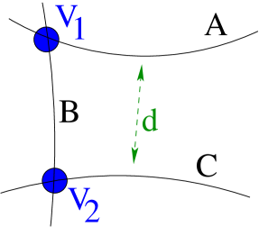
Figure 1: Schematic description of how the triangle inequality is violated in the track clustering problem.

Theorem: The triangle inequality does not generally hold for the minimum distances between a set of $n$ tracks.

Proof: Let $A,B,C$ denote three tracks. Let $A$ and $B$ share one common vertex $V_{1}$; let further $B$ and $C$ also share one common vertex $V_{2}$. Then:

$$\overline{AB}=\epsilon,\overline{BC}=\epsilon,\overline{AC}=d\gg\epsilon$$

$$\rightarrow\overline{AB}+\overline{BC}\ll\overline{AC}\hskip 5.69054ptq.e.d.$$ (3)

This means that the choice $d(\alpha,\beta)=\text{min}(s)$ would cluster A, B and C into a single vertex. We can therefore safely discard single linkage from the list of promising algorithms.

Until now the best results were obtained with the choice $d(\alpha,\beta)=\text{max}(s)$, i.e. with a complete linkage procedure.

An alternative to the above metrices is of course to fit vertices for each cluster with more than one track, and use these vertices as “representatives” of the cluster.

III.1 Finding-Thru-Fitting

The most mature algorithm in CMS is the “principal vertex reconstructor”, also known as the “finding-thru-fitting” method. It is a divisive method that internally uses a fitter and a track-to-vertex compatibility estimator to decide which tracks are to be discarded at each iteration step. The maturity of the implementation and the algorithmic simplicity make it an ideal baseline for performance evaluation.

III.2 Apex points

In order to overcome the topological problems described in section 3, we conceived another approach: the apex point formalism. The main concept is that the tracks are substituted by representative points, the apex points. These points should fully represent the tracks with respect to the vertex finding problem at hand. The space that the apex points are defined in can have any dimension; it must only be equipped with a proper metric fulfilling the triangle inequality. Our current implementation produces three-dimensional points in a Euclidean space, together with a 3x3 error matrix. Note that the apex-point-to-track mapping needs not be unique; it may very well be necessary that $n$ apex points, $n>1$, represent one track.

One can of course also formulate hierarchic clustering methods on top of the apex points.

III.3 Apex point finders

An algorithm that searches for such representative “apex” points is called an apex point finder. Since these finders operate on the points of closest approach, they can be formulated as generic pattern recognition problems in one dimension (i.e. along the tracks). Thus the set of potential apex point finding algorithms is huge; a systematic effort to choose algorithms that satisfy our needs is an ongoing process. So far we have only investigated a few simple methods:

• The HSM (half sample mode) finder iteratively calls an LMS estimator on the points of closest approach.

• The MTV (minimal two values) finder looks for the two adjacent points of closest approach whose sum of distances to their counterparts on the other tracks is minimal.

• The MAMF (minimum area mode) finder looks for the two adjacent points whose sum of distances to their counterparts times their distance is minimal.

Future research will try more sophisticated algorithms such as a deterministic annealing anneal , oldanneal method, or a gravitational clusterer gravity .

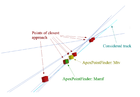
Figure 2: Two apex point finders at work.

III.4 Global association criterion

The weights that have been introduced for the adaptive fitting method (see section 1) can also be used to define a global “plausibility” criterion of the result of a vertex reconstructor. With $m$ being the total number of tracks and $n$ being the number of vertices we define the global association criterion (GAC) by:

$$p=\frac{1}{n\cdot m}\sum_{i=1}^{\text{m}}\sum_{j=1}^{\text{n}}p_{ij}$$

where

$$p_{ij}=\left\{\begin{tabular}[]{lc}$1-w_{ij}$&if $i\in j$\\ $w_{ij}$&otherwise\end{tabular}\right.$$

and $w_{ij}$ is the weight $w_{i}$ (1) of track $i$ with respect to vertex $j$.

The most important open question with respect to this criterion is how it relates to the “Minimum Message Length” mel . Can the information theoretic limit of the vertex finding task be formulated in terms of the GAC?

The potential uses of such a criterion are manifold:

• Exhaustive vertex finding algorithm. All combinations of track clusters could at least in principle be iterated through, then one can decide for the smallest GAC found.

• Stopping condition. The GAC could also serve as a stopping condition in a wide range of algorithms.

• Super finder algorithms. One could also use it to resolve ambiguities. More than one vertex reconstructors could be used on one event, the GAC could then decide for the “better” solution.

Clearly, some more research in this direction will have to be done.

III.5 Learning algorithms

“Learning algorithms” can easily be formulated on top of the apex points; some can also work on the distance matrix itself. Good candidates for such algorithms are:

• Vector quantisation or the k-means algorithm, which have dynamic vertex candidates (“prototypes”) that are attracted by the apex points.

• Potts neurons potts or the super-paramagnetic clustering algorithm spc ; these algorithms attribute a spin-state or a mathematical equivalent to every apex point. Spin-spin correlations together with an annealing schedule will then make sure that similar apex points are described by the same spin vector.

• Deterministic annealing anneal ; this method formulates the clustering problem as a thermodynamic system with phase transitions, each transition introducing a new separate cluster of apex points.

III.6 Simulation experiment

We compared one of our algorithms with two standard vertex finding procedures: the PVR (see section III.1) and the so-called D0Phi method d0phi , cdf – a special purpose algorithm based on the impact parameters of the tracks at the beamline. As a novel method to compare with we chose an agglomerative clusterer with a vertex fits as “representative points”, as it was explained in the last paragraph of section III. Our testing was done with 1000 Monte Carlo 50 GeV $b\bar{b}$ events, generated with the CMSIM simulation program cmsim . Before the actual comparison all algorithms were automatically fine-tuned to maximize the following “score function”:

$$\text{Score}\equiv 10\cdot\text{Eff}_{\text{Prim}}\cdot\text{Eff}_{\text{Sec}}\cdot\text{Pur}_{\text{Prim}}^{0.25}\cdot\text{Pur}_{\text{Sec}}^{0.25}\cdot$$

$$\text{AssEff}_{\text{Prim}}^{0.25}\cdot\text{AssEff}_{\text{Sec}}^{0.25}\cdot\left(1-\text{Fake}\right)^{0.5}$$

“Eff”, “Pur”, “AssEff”, and “Fake” denote the performance estimators described in pascal-chep2003 ; “Prim” denotes primary vertices, “Sec” stands for secondardy vertices.

III.7 Results

In the inclusive secondary vertex finding scenario, the agglomerative fitting procedure finds up to 80 percent of the secondary vertices, as opposed to the 50 – 60 percent found by older algorithms. Note that the D0Phi algorithm is not intended to find any primary vertices, hence the total score parameter is meaningless. See figure 3 for the complete comparison.

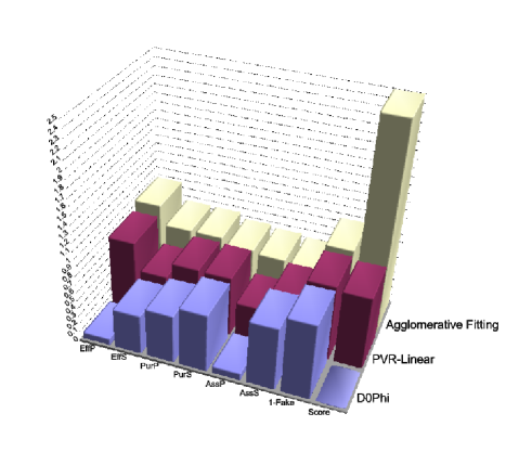
Figure 3: Analysis of performance: one novel agglomerative finder compared to older vertex finding algorithms. The agglomerative method has a much higher secondary vertex finding efficiency, while it reports about the same fake rate.

IV CONCLUSIONS

We have reached a good understanding of the robustification methods of the classical LS vertex fitters. We suggest that the adaptive method be used as the new default fitting procedure for CMS and possibly other experiments as well. Surely, we still lack such an exhaustive understanding in the case of the much more complex task of vertex finding, although here we were able to exclude certain classes of algorithms on the basis of purely theoretic considerations. Our first results are most promising; we can quite clearly demonstrate that with respect to e.g. secondary vertex finding classical methods such as the “finding-thru-fitting” algorithm can be surpassed by far. Future research will mainly focus on three areas:

• apex point finding algorithms,

• “learning” algorithms,

• the global association criterion and its implications.

References

- (1) T. Boccali et al., Vertex reconstruction framework and its implementation for CMS, these proceedings.
- (2) R. Frühwirth et al., New developments in vertex reconstruction for CMS, NIMA 502 (2003) 699–701.
- (3) K. Van Driessen and P.J. Rousseuw, Computing LTS regression for large data sets (1999) University of Antwerp.
- (4) J. D’Hondt, R. Frühwirth, P. Vanlaer, and W. Waltenberger, CMS Note, in preparation.
- (5) G. Segneri, F. Palla, Lifetime based -tagging with CMS, CMS Note 2002/046.
- (6) F.Abe et al. [CDF Collaboration], Evidence For Top Quark Production In Anti-P P Collisions At S**(1/2) = 1.8 TeV, Phys. Rev. D50 (1994) 2966.
- (7) K. Rose, Deterministic annealing for clustering, compression, classification, regression and related optimization problems, Proc. IEEE, vol. 86, num. 11 (1998) 2210–2239.
- (8) K. Rose, E. Gurewitz, and G. C. Fox, Statistical mechanics and phases transitions in clustering, Phys. Rev. Lett., vol. 65, num. 8 (1990) 945–948.
- (9) S. Kundu, Gravitational clustering: a new approach based on the spatial distribution of the points, Pattern Recognition 32 (1999) 1149–1160.
- (10) C. S. Wallace, and D. L. Dowe, Minimum Message Length and Kolmogorov Complexity, Computer Journal, vol. 42, Issue 4 (1999) 270–283.
- (11) M. Bengtsson and P. Roivainen, Using the Potts glass for solving the clustering problem, International Journal of Neural Systems, vol. 6, num. 2 (1995) 119–132.
- (12) M. Blatt, S. Wiseman and E. Domany, Super-paramagnetic clustering of data, Phys. Rev. Lett. 76 (1996) 3251–3254.
- (13) C. Charlot et al., CMS Simulation Facilities, CMS TN 93-63, CERN, Geneva, 1993.