Nonlinear surface waves in left-handed materials

Abstract

We study both linear and nonlinear surface waves localized at the interface separating a left-handed medium (i.e. the medium with both negative dielectric permittivity and negative magnetic permeability) and a conventional (or right-handed) dielectric medium. We demonstrate that the interface can support both TE- and TM-polarized surface waves–surface polaritons, and we study their properties. We describe the intensity-dependent properties of nonlinear surface waves in three different cases, i.e. when both the LH and RH media are nonlinear and when either of the media is nonlinear. In the case when both media are nonlinear, we find two types of nonlinear surface waves, one with the maximum amplitude at the interface, and the other one with two humps. In the case when one medium is nonlinear, only one type of surface wave exists, which has the maximum electric field at the interface, unlike waves in right-handed materials where the surface-wave maximum is usually shifted into a self-focussing nonlinear medium. We discus the possibility of tuning the wave group velocity in both the linear and nonlinear cases, and show that group-velocity dispersion, which leads to pulse broadening, can be balanced by the nonlinearity of the media, so resulting in soliton propagation.

I Introduction

Novel physical effects in dielectric media with both negative permittivity and negative permeability were first analyzed theoretically by Veselago Veselago:1967-517:UFN who predicted a number of unusual phenomena including, for example, negative refraction of waves. Such media are usually known as left-handed (LH) media since the electric and magnetic fields form a left handed set of vectors with the wave vector. The physical realization of such LH media was demonstrated only recently Smith:2000-4184:PRL for a novel class of engineered composite materials, now called LH metamaterials. Such LH materials have attracted attention not only due to their recent experimental realization and a number of unusual properties observed in experiment, but also due to the expanding debates on the use of a slab of a LH metamaterial as a perfect lens for focusing both propagating and evanescent waves Venema:2002-119:Nature .

The concept of a perfect lens was first introduced by Pendry Pendry:2000-3966:PRL , who suggested the idea that a slab of a lossless negative-refraction material can be used for creating a perfect image of a point source. Although the concept of a perfect lens is a result of an ideal theoretical model employed in the analysis Pendry:2000-3966:PRL , the resolution limit of a LH slab was shown to be independent of the wavelength of the electromagnetic wave (but can be determined by other factors including losses, spatial dispersion, and others), so that the resolution can be indeed much better than the resolution of a conventional lens Luo:2002-201104:PRB .

The improved resolution of a LH slab and the corresponding amplification of evanescent modes even in a lossy LH material, can be understood from simple physics. Indeed, the near field of an image, which can not be focused by a normal lens, can be transferred through the slab of a LH material due to the excitation of surface waves (or surface polaritons) at both interfaces of the slab. Therefore, as the first major step in the understanding of the amplified transmission of the evanescent waves, as well as other unusual properties of the LH materials, it is important to study the properties of different types of surface wave that can be excited at the interfaces between LH and conventional (or right-handed, RH) media. Some preliminary studies in this direction included calculation of the linear dispersion properties of modes localized at a single interface or in a slab of LH material Ruppin:2000-61:PLA ; Pendry:1998-10096:PRL ; Bespyatyh:2001-2043:FTT ; Haldane:cond-mat/0206420 ; Shadrivov:2003-057602:PRE .

In this paper, we present a comprehensive study of the properties of both linear and nonlinear surface waves at the interface between semi-infinite materials of two types, left- and right-handed ones, and demonstrate a number of unique features of surface waves in LH materials. In particular, we show the existence of surface waves of both TE and TM polarizations, a specific feature of the RH/LH interfaces. We study in detail TE-polarized nonlinear surface waves and suggest an efficient way for engineering the group velocity of surface waves using the nonlinearity of the media. The dispersion broadening of the pulse can be compensated by the nonlinearity, thus leading to the formation of surface-polariton solitons at the RH/LH interfaces with a distinctive vortex-like structure of the energy flow. We must note here, that the presented study is based on the effective medium approximation, which treats the LH materials as homogeneous and isotropic. It can be applied to the manufactured metamaterials, which possess negative dielectric permittivity and negative permeability in the microwave frequency range, when the characteristic scale of the variation of the electromagnetic field (e.g. a field decay length and a wavelength of radiation) is much higher, than the period of the metamaterial. The possibility of preparing isotropic LH materials was studied in Shelby:2001-489:APL , where the isotropy of the composite in 2D has been shown. To obtain a negative-refraction material in optics it is suggested that metallic nanowires are used Ref. Podolskiy:2002-65:JNOM . Also, we note that losses is an intrinsic feature of LHM. However, the study of the effect of losses on the guided waves is not in the scope of the present paper.

The paper is organized as follows. In Sec. II we study the properties of surface waves in the linear regime. We consider the most general case of an interface between linear RH and LH media, and present a classification of TE- and TM-polarized surface waves localized at the interface. Section III is devoted to the study of the structure and general properties of nonlinear surface waves. We describe the intensity-dependent properties of TE-polarized surface waves in three possible cases. In the first case, we assume that both the LH and RH media are nonlinear. In the second case, the LH medium is nonlinear, but the RH medium is assumed to be linear. In the third case, the RH medium is considered to be nonlinear while the LH medium remains linear. In all these cases, we take the nonlinear medium have an intensity-dependent Kerr-like dielectric permittivity. In Section IV, we study the frequency dispersion of nonlinear surface waves. In particular, we demonstrate that the group velocity of surface waves can effectively be engineered by using the intensity-dependent dispersion. A detailed analysis is carried out for the example of nonlinear RH and linear LH media. Finally, in section V we describe the properties of nonlinear localized modes propagating along the interface, and predict the existence of surface polariton solitons.

II Linear surface waves

II.1 Model

Linear surface waves are known to exist, under certain special conditions, at an interface separating two different isotropic dielectric media. In particular, the existence of TM-polarized surface waves requires that the dielectric constants of two dielectric materials separated by an interface have different signs, whilst for TE-polarized waves the magnetic permeability of the materials should be of different signs (see, e.g. Ref. Nkoma:1974-3547:JPC ; Boardman:EMSurfaceModes and references therein). Materials with negative $\epsilon$ are readily available (e.g., metals excited below a critical frequency), whilst materials with negative $\mu$ were not known until recently. This explains why only TM-polarized surface waves have been of interest over the last few decades.

In this paper, we consider an interface between the RH (medium 1) and LH (medium 2) semi-infinite media, as shown in the inset of Fig. 1. The propagation of monochromatic waves with the frequency $\omega$ is governed by the scalar wave equation, which for the case of the TE waves is written for the y-component of the electric field,

$$\left[\frac{\partial^{2}}{\partial z^{2}}+\frac{\partial^{2}}{\partial x^{2}}+\frac{\omega^{2}}{c^{2}}\epsilon(x)\mu(x)-\frac{1}{\mu(x)}\frac{\partial\mu(x)}{\partial x}\frac{\partial}{\partial x}\right]E_{y}=0.$$ (1)

In the case of the TM waves, the scalar wave equations is written for the y-component of magnetic field,

$$\left[\frac{\partial^{2}}{\partial z^{2}}+\frac{\partial^{2}}{\partial x^{2}}+\frac{\omega^{2}}{c^{2}}\epsilon(x)\mu(x)-\frac{1}{\epsilon(x)}\frac{\partial\epsilon(x)}{\partial x}\frac{\partial}{\partial x}\right]H_{y}=0.$$ (2)

In Eqs. (1) and (2), the functions $\epsilon(x)$ and $\mu(x)$ are dielectric permittivity and magnetic permeability in a bulk medium, respectively; $\omega$ is the angular wave frequency, and $c$ is the speed of light in vacuum. The nonzero components of the magnetic field and of the electric field are found from the Maxwell’s equations, i.e. for TE waves

$$H_{z}=-\frac{ic}{\omega\mu}\frac{\partial E_{y}}{\partial x};\;\;H_{x}=\frac{ic}{\omega\mu}\frac{\partial E_{y}}{\partial z},$$ (3)

and for TM waves

$$E_{z}=\frac{ic}{\omega\epsilon}\frac{\partial H_{y}}{\partial x};\;\;E_{x}=-\frac{ic}{\omega\epsilon}\frac{\partial H_{y}}{\partial z},$$ (4)

respectively. Solutions of Eqs. (1) and (2) in each linear medium for localized modes, i.e. those propagating along the interface and decaying in transverse direction, have the form

$$(E_{y},H_{y})=A_{0}e^{ihz-\kappa_{1,2}|x|},$$ (5)

where $A_{0}$ is the wave amplitude at the interface, $h$ is a propagation constant,

$$\kappa_{1,2}=\left[h^{2}-\epsilon_{1,2}\mu_{1,2}\left(\frac{\omega}{c}\right)^{2}\right]^{1/2}$$

is the transverse wave number which characterizes the inverse decay length of the surface wave in the corresponding medium.

It follows from Eqs. (1) and (2) that the tangential components of the electric and magnetic fields change continuously at the interface between two media. These conditions give the dispersion relations for surface waves Ruppin:2000-61:PLA ,

$$\frac{\kappa_{1}}{\mu_{1}}+\frac{\kappa_{2}}{\mu_{2}}=0,$$ (6)

and

$$\frac{\kappa_{1}}{\epsilon_{1}}+\frac{\kappa_{2}}{\epsilon_{2}}=0,$$ (7)

for the cases of the TE- and TM-polarized surface waves, respectively.

II.2 Properties of surface waves

For the analysis presented below, it is convenient to rewrite the dispersion relations (6) and (7) in the following form,

$$h^{2}=\epsilon_{1}\mu_{1}\left(\frac{\omega}{c}\right)^{2}\frac{Y(Y-X)}{(Y^{2}-1)},$$ (8)

and

$$h^{2}=\epsilon_{1}\mu_{1}\left(\frac{\omega}{c}\right)^{2}\frac{X(X-Y)}{(X^{2}-1)},$$ (9)

respectively, where we introduced the dimensionless normalized ratios $X=|\epsilon_{2}|/\epsilon_{1}$ and $Y=|\mu_{2}|/\mu_{1}$ which characterize the relative properties of the media creating the interface. The existence regions for surface waves can be determined from the condition of surface wave localization, i.e. when the transverse wave numbers $\kappa_{1,2}$ are real, $h>\max{\{\omega\epsilon_{1}\mu_{1}/c,\;\omega\epsilon_{2}\mu_{2}/c}\}$. Existence regions for both polarizations of surface wave are presented on the parameter plane $(X,Y)$ in Fig. 1. Along with the polarization, we determine the type of the wave as forward or backward, as discussed below in Sec. II.3. We note that there exist no regions where both TE- and TM-polarized waves co-exist simultaneously, but both types of surface wave can be supported by the same interface for different parameters, e.g. for different frequencies.

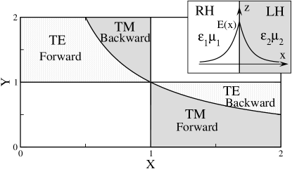
Figure 1: Existence regions of surface waves on the parameter plane $(X,Y$), where $X=|\epsilon_{2}|/\epsilon_{1}$ and $Y=|\mu_{2}|/\mu_{1}$. The inset shows the problem geometry.

Figure 2: Dispersion curves of the TE-polarized surface waves, for different values of $\epsilon_{1}$, shown for the normalized values $\bar{\omega}=\omega/\omega_{p}$ are $\bar{h}=hc/\omega_{p}$. Dotted curves marks the dependence $\bar{h}=\bar{\omega}\sqrt{\epsilon_{2}\mu_{2}}$. Dashed line is the critical frequency $\omega_{1}$.

One of the distinctive properties of the LH materials which has been demonstrated experimentally is their specific frequency dispersion. To study the dispersion of the corresponding surface waves, it is necessary to select a particular form of the frequency dependence of the dielectric permittivity and magnetic permeability of the LH medium. A negative dielectric permittivity is selected in the form of the commonly used function for plasmon investigations Boardman:EMSurfaceModes and a negative permeability is constructed in an analogous form (see, e.g. Ref. Ruppin:2000-61:PLA ), i.e.

$$\epsilon_{2}(\omega)=1-\frac{\omega_{p}^{2}}{\omega^{2}},\;\;\;\;\;\mu_{2}(\omega)=1-\frac{F\omega^{2}}{\omega^{2}-\omega_{r}^{2}},$$ (10)

where losses are neglected, and the values of the parameters $\omega_{p}$, $\omega_{r}$, and $F$ are chosen to fit approximately to the experimental data Smith:2000-4184:PRL : $\omega_{p}/2\pi=10$ GHz, $\omega_{r}/2\pi=4$ GHz, and $F=0.56$. For this set of parameters, the region in which permittivity and permeability are simultaneously negative is from 4 GHz to 6 GHz.

The dispersion curves of the TE-polarized surface wave (or surface polariton) calculated with the help of Eq. (10) are depicted in Fig. 2 on the plane of the normalized parameters $\bar{\omega}=\omega/\omega_{p}$ and $\bar{h}=hc/\omega_{p}$. We note that the structure of the dispersion curves for surface waves depends on the relation between the values of the dielectric permittivities of the two media at the characteristic frequency, $\omega_{1}$, at which the absolute values of magnetic permeabilities of two media coincide, $\mu_{1}=|\mu_{2}(\omega_{1})|$. The corresponding curve in Fig. 2 is monotonically decreasing for $\epsilon_{1}>|\epsilon_{2}(\omega_{1})|$, but it is monotonically increasing otherwise, i.e. for $\epsilon_{1}<|\epsilon_{2}(\omega_{1})|$. Only the first case was identified in the previous analysis reported in Ref. Ruppin:2000-61:PLA . The change of the slope of the curve (the slope of the dispersion curve represents the group velocity) with the variation of the dielectric permittivity of the RH medium can be used for group velocity engineering, which we discuss in Sec. IV.

The critical value of dielectric permittivity $|\epsilon_{2}(\omega_{1})|$ for the case of a nonmagnetic RH medium ($\mu_{1}=1$) is found from the dispersion relations (6) and (10), and it has the form

$$\epsilon_{c}=|\epsilon_{2}(\omega_{1})|=\left(1-\frac{F}{2}\right)\left(\frac{\omega_{p}}{\omega_{r}}\right)^{2}-1$$ (11)

For the parameters specified above, this critical value is $\epsilon_{c}=3.5$.

The change of the dispersion curve from monotonically increasing to monotonically decreasing, shown in Fig. 2, is connected with a change in the direction of the total power flow in the wave, as discussed below.

II.3 Energy flow near the interface

The energy flow is described by the Poynting vector, which defines the energy density flux averaged over the period $T=2\pi/\omega$, and can be written in the form

$${\bf S}=\frac{c}{8\pi}\rm{Re}\left[{\bf E}\times{\bf H}^{*}\right],$$ (12)

where ${\bf E},{\bf H}$ are the complex envelopes of the electric field and magnetic field of a surface wave, respectively, and the asterisk stands for the complex conjugation.

A uniform surface wave propagating along the interface has only one non-zero component of the averaged Poynting vector, $|{\bf S}|=|S_{z}|$. The energy flux in the RH and LH media is an integral of the Poynting vector over the corresponding semi-infinite spatial region,

$$P_{1}=\int_{-\infty}^{0}S_{z}\,dz=\frac{Bh}{\kappa_{1}}\left\{\begin{array}[]{rcl}1/\mu_{1};\;\mbox{for TE},\\ 1/\epsilon_{1};\;\mbox{for TM},\end{array}\right.$$ (13)

$$P_{2}=\int_{0}^{\infty}S_{z}\,dz=\frac{Bh}{\kappa_{2}}\left\{\begin{array}[]{rcl}1/\mu_{2};\;\mbox{for TE},\\ 1/\epsilon_{2};\;\mbox{for TM},\end{array}\right.$$ (14)

where the constant $B=c^{2}A_{0}^{2}/16\pi\omega$. We note that the electromagnetic energy flow is in opposite directions at either side of the interface, as was also predicted in  Nkoma:1974-3547:JPC for TM polarized waves. The total energy flux in the forward $z$-direction is defined as the sum, $P=P_{1}+P_{2}$, and it is found as

$$P=\left(1-XY\right)\frac{Bh\omega^{2}\epsilon_{1}\mu_{1}}{\kappa_{1}\kappa_{2}c^{2}}\left\{\begin{array}[]{rcl}\left(1+Y^{2}\right)/\left[Y(\mu_{1}\kappa_{1}-\mu_{2}\kappa_{2})\right],\\ \left(1+X^{2}\right)/\left[X(\epsilon_{1}\kappa_{1}-\epsilon_{2}\kappa_{2})\right],\end{array}\right.$$ (15)

for the TE and TM waves, respectively. The total energy flux is positive for $XY<1$, and negative for $XY>1$. The surface waves are forward or backward, respectively. The corresponding types of surface waves determined from this analysis are labelled in Fig. 1.

III Nonlinear surface waves

III.1 Nonlinear LH/RH interface

Nonlinear surface waves at an interface separating two conventional dielectric media have been analyzed extensively for several decades starting from the pioneering paper Litvak:1968-1911:IVR . In brief, one of the major findings of those studies is that the TE-polarized surface waves can exist at the interface separating two RH media provided that at least one of these is nonlinear, but that no surface waves exist in the linear limit.

In this section, we study TE-polarized nonlinear surface waves assuming that both media are nonlinear, i.e. they display a Kerr-type nonlinearity in their dielectric properties, namely

$$\epsilon_{1,2}^{NL}=\epsilon_{1,2}+\alpha_{1,2}|E|^{2},$$ (16)

where the first term characterizes the linear properties, i.e. those in the limit of vanishing wave amplitude.

First, we should mention that the recent systematic study of nonlinear properties of metallic composites Zharov:2003-037401:PRL suggested the possibility of hysteresis-type nonlinear effects in a structure consisting of arrays of split-ring resonators (SRRs) and wires embedded in a nonlinear dielectric medium. Such effects can also be caused by a nonlinear dielectric material placed in the slits of the SRRs, which results in an intensity-dependent capacitance of the slit. These hysteresis effects can be avoided if the structure is filled by a nonlinear dielectric material except in the SRR slits. In what follows, we consider such composite structures for which the nonlinear properties can be characterized by Eq. (16) valid far from the resonances.

For a conventional (or right-handed) dielectric medium, positive $\alpha_{1}$ corresponds to a self-focusing nonlinear material, whilst negative $\alpha_{1}$ characterizes defocusing effects in the beam propagation. However, this classification becomes reversed in the case of LH materials and, for example, a self-focusing LH medium corresponds to negative $\alpha_{2}$. Indeed, taking into account relation (16), we rewrite Eq. (1) for the case of the TE-polarized wave in nonlinear media as follows,

$$\frac{\partial^{2}E}{\partial z^{2}}+\frac{\partial^{2}E}{\partial x^{2}}+\left(\frac{\omega}{c}\right)^{2}\left(\epsilon\mu+\mu\alpha|E|^{2}\right)E=0.$$ (17)

According to Eq. (17), the sign of the product $\mu\alpha$ determines the type of nonlinear self-action effects which occur. Therefore, in a LH medium with negative $\mu_{2}$ all nonlinear effects are opposite to those in RH media with positive $\mu_{1}$, for the same $\alpha$. Below, we assume for definiteness that both LH and RH materials possess self-focusing properties, i.e. $\alpha_{1}>0$ and $\alpha_{2}<0$.

We look for the stationary solutions of Eq. (17) in the form $E_{1,2}(x,z)=\Psi_{1,2}(x)\exp{(ihz)}$. Then, the profiles of the spatially localized wave envelopes $\Psi_{1,2}(x)$ are found as Zakharov:1972-62:JETP

$$\Psi_{1,2}(x)=\left(\eta_{1,2}\sqrt{2/\alpha_{1,2}\mu_{1,2}}\right)\;{\rm sech}[\eta_{1,2}(x-x_{1,2})],$$ (18)

where $\eta_{1,2}=\kappa_{1,2}c/\omega$ are normalized transverse wave numbers, $x_{1,2}$ are centers of the sech-functions which should be chosen to satisfy the continuity of the tangential components of the electric and magnetic fields at the interface. These conditions can be presented in the form of two transcendental equations,

$$\tanh^{2}{(\eta_{1}x_{1})}=\left(1-\frac{\alpha_{1}\mu_{1}\eta_{2}^{2}}{\alpha_{2}\mu_{2}\eta_{1}^{2}}\right)\left(1-\frac{\alpha_{1}\mu_{2}}{\alpha_{2}\mu_{1}}\right)^{-1},$$ (19)

and

$$\frac{\eta_{2}}{\mu_{2}}\tanh{(\eta_{2}x_{2})}=\frac{\eta_{1}}{\mu_{1}}\tanh{(\eta_{1}x_{1})}.$$ (20)

Note, that if the parameters $(x_{1},x_{2})$ correspond to one of the solutions of the equation, then $(-x_{1},-x_{2})$ gives another solution. Two waves described by these solutions have the same wave number, but they correspond to different transverse structures of the surface wave, one of which has a maximum of the intensity at the interface, and the other one that has two humps shifted into the media.

In a degenerate case, when $(\alpha_{1},\mu_{1},\epsilon_{1})=(\left|\alpha_{2}\right|,\left|\mu_{2}\right|,\left|\epsilon_{2}\right|)$, the system has an infinite number of solutions. Indeed, any $(x,-x)$ pair will describe a stationary solution for the surface wave. Such waves have a zero total energy flux because of the symmetry of the solution.

The energy flow in this wave can be written in the form

$$P=P_{0}\gamma\left[\frac{\eta_{1}\alpha_{2}\mu_{2}}{\alpha_{1}\mu_{1}^{2}}+\frac{\eta_{2}}{\mu_{2}}+\frac{\eta_{1}}{\mu_{1}}\left(1-\frac{\alpha_{2}\mu_{2}}{\alpha_{1}\mu_{1}}\right)\tanh{(\eta_{1}x_{1})}\right],$$ (21)

where $P_{0}=c^{2}/4\pi\omega\alpha_{2}\mu_{2}$, and $\gamma=hc/\omega$ is the normalized wave number. We now consider the surface waves in the non-degenerate case when only $\alpha_{1}=\left|\alpha_{2}\right|$. The dependence of the normalized energy flux $P/P_{0}$ on the parameter $\gamma$ is shown in Fig. 3 for the cases when linear waves are forward or backward, respectively. Corresponding transverse wave structures are shown in the insets.

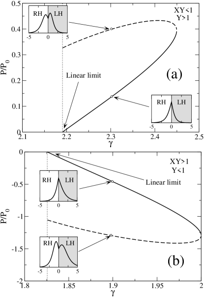
Figure 3: Normalized energy flux vs. normalized wavenumber $\gamma=hc/\omega$ for the nonlinear surface waves in two cases: (a) $XY<1$, $Y>1$, and (b) $XY>1$, $Y<1$. Solid curve corresponds to a one-humped structure, dashed – double-humped structure. The insets shows the structure of the surface waves at the points indicated by arrows. Dotted lines denote the linear surface wave wavenumber.

The linear limit corresponds to the case $P\to 0$ when $x_{1}\to+\infty$ and $x_{2}\to-\infty$. Moving along the curves, the centers of the sech-functions move toward the interface and at the point with $dP/d\gamma=\infty$, $x_{1}=x_{2}=0$, and from that point along the dashed line $x_{1}\to-\infty,x_{2}\to+\infty$, thus revealing the two-humped transverse structure of the surface wave. Note that the forward (backward) wave in the linear case remains forward (backward) in the nonlinear case, i.e. the type of the mode is determined by the linear parameters of the system and can be found using the diagram in Fig. 1.

III.2 Nonlinear LH/linear RH interface

Next, we consider surface waves propagating along an interface between linear RH and nonlinear LH media (see the inset in Fig. 4) having the negative nonlinear coefficient $\alpha_{2}$ and, thus, displaying the self-focusing properties. The transverse structure of the stationary surface wave has the form:

$$\Psi(x)=\left\{\begin{array}[]{lr}E_{0}\exp{(\eta_{1}x)},\;x<0,\\ \left(2/\alpha_{2}\mu_{2}\right)^{1/2}\eta_{2}\,{\rm sech}\left[\eta_{2}(x-x_{0})\right],\;x>0,\end{array}\right.$$ (22)

where $E_{0}$ and $x_{0}$ are two parameters which should be determined from the continuity conditions at the interface for the tangential components of the electric and magnetic fields,

$$\tanh{\left(\eta_{2}x_{0}\right)}=\mu_{2}\eta_{1}/(\mu_{1}\eta_{2}),$$

$$E_{0}=(2/\alpha_{2}\mu_{2})^{1/2}\eta_{2}\,{\rm sech}(\eta_{2}x_{0}).$$ (23)

Analyzing the relations (III.2), we find that a surface wave always has the maximum of field intensity at the interface. This is in a sharp contrast to the nonlinear surface waves excited at the interface separating two RH media, when the electric field has maximum shifted into a self-focusing nonlinear medium Boardman:1985-1701:JQEL .

The corresponding nonlinear dispersion relation of the surface waves is found in the form

$$\frac{\eta_{1}}{\mu_{1}}+\frac{\eta_{2}}{\mu_{2}}\left(1-\frac{A_{1}^{2}}{\eta_{2}^{2}}\right)^{1/2}=0,$$ (24)

where $A_{1}=E_{0}(\alpha_{1}\mu_{1}/2)^{1/2}$ is the normalized electric field amplitude at the interface. Equation (24) reduces to the linear dispersion relation (6) in the small-amplitude limit, i.e. when $A_{1}\to 0$.

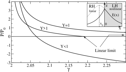
Figure 4: Normalized energy flux vs normalized wavenumber $\gamma=hc/\omega$ for the nonlinear surface waves at the nonlinear LH/Linear RH interface. Surface waves can be both forward (positive energy flux) and backward (negative energy flux). The inset shows the geometry of the problem. The solid line shows the transverse wave profile, dotted line shows the continuation of the solution in nonlinear medium (22) to the linear medium, dashed line indicates the position of the center $x_{0}$ of the sech - function.

The energy flux $P$ associated with the nonlinear surface wave can be calculated in the form

$$P=P_{0}\gamma\eta_{2}\left(1+\frac{\mu_{2}\eta_{1}}{\mu_{1}\eta_{2}}\right)\left[\frac{2}{\mu_{2}}+\frac{\eta_{2}}{\eta_{1}\mu_{1}}\left(1-\frac{\mu_{2}\eta_{1}}{\mu_{1}\eta_{2}}\right)\right],$$

where $P_{0}$ is defined above.

As an example, we consider the case $XY<1$ for which, as we have shown above, only forward surface waves can exist at the interface between two linear media. However, nonlinear surface waves can be either forward or backward, as demonstrated in Fig. 4. For $Y<1$, there exists no linear limit for the existence of the surface waves, while in other two regions the results for linear surface waves are recovered in the limit $P\to 0$. The point on the curve corresponding to $P=0$ in the case $Y<1$ describes the wave of finite amplitude in which the energy flows on either side of the interface are balanced. Such a wave does not exist in the linear limit.

III.3 Linear LH/nonlinear RH interface

Finally, we consider the case when the LH material is linear, while the RH medium is nonlinear. In such a geometry, the dispersion relation for the TE-polarized waves has the form

$$\frac{\eta_{2}}{\mu_{2}}+\frac{\eta_{1}}{\mu_{1}}\left(1-\frac{A_{2}^{2}}{\eta_{1}^{2}}\right)^{1/2}=0,$$ (25)

where $A_{2}=E_{0}\sqrt{\alpha_{2}\mu_{2}/2}$ is the normalized amplitude of the electric field at the interface.

The dependence of the normalized energy flux on the wave number of the surface wave is shown in Fig. 5 for $XY>1$. In contrast to the linear waves, the nonlinear surface waves can be either forward or backward (see Fig. 1). In analogy with the case $Y<1$ for the nonlinear LH/linear RH interface, it can be shown that there exists no small-amplitude limit for the nonlinear surface waves for $Y>1$ . For $XY<1$ only forward travelling waves exist when $Y>1$, reproducing the property of the corresponding linear waves.

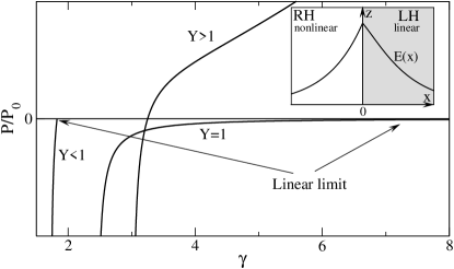
Figure 5: Normalized energy flux vs normalized wavenumber $\gamma=hc/\omega$ for the nonlinear surface waves at the linear LH/nonlinear RH interface. Surface waves can be either forward (positive energy flux) or backward (negative energy flux). The inset shows the geometry of the problem.

IV Frequency dispersion of nonlinear surface waves

We have demonstrated in Sec. II.2 that the frequency dispersion of surface waves depends on the dielectric permittivity of the RH medium (see Fig. 2). These results suggest that the dispersion type can be switched between normal and anomalous if the RH medium is nonlinear.

To demonstrate this property, we study the properties of nonlinear surface waves near the critical point and select $\epsilon_{1}=3.4$, in order to stay just below the critical value $\epsilon_{c}$ corresponding to the linear case. It should be mentioned here that although the negative permeability of the LH composite material is necessary for the existence of TE surface waves in the present model, it has been shown Maradudin:1981-341:ZPCM that TE surface waves do exist at the interface between a RH nonlinear plasma and a RH nonlinear dielectric medium with a constant zero-field permittivity, provided that the nonlinear parameter in the plasma exceeds that in the dielectric medium. In that case, since $\mu=1$ in both media, it has also been shown Maradudin:1981-341:ZPCM that the relation for wave intensity at the boundary and the frequency are independent of the wave number. In the present case, where the LH composite material has a permeability not equal to unity, this result is no longer valid. In our problem, Eq. (25) provides a dependence between the three variables $h$, $A_{2}$ and $\omega$, so that the wave intensity at the boundary depends on both $h$ and $\omega$.

As was shown for the case of linear surface waves, a change of the slope of the dispersion curve takes place at the critical value of dielectric permittivity of the RH medium (11). In the nonlinear case, the dielectric permittivity of the RH medium depends on the field intensity and, in particular, it exceeds the critical value when the wave amplitude $A_{2}$ becomes larger than the threshold value $A_{2c}$ given by the equation

$$A_{2c}^{2}=\left(\frac{\omega_{p}}{\omega_{r}}\right)^{2}\left(1-\frac{F}{2}\right)-\left(1+\epsilon_{1}\right).$$ (26)

For the media parameters corresponding to Fig. 2, equation (26) gives: $A_{2c}=0.3162$. Figure 6 shows the dispersion curves for three different wave amplitudes. As was shown in Sec. II.2, the frequency dispersion is normal for the wave amplitudes below the critical value (26), and it is negative, otherwise. One can also notice from Fig. 6 that the existence region for surface waves depends on the wave amplitude $A_{2}$. In Fig. 7 we present this region of wave existence on the plane of the wave amplitude and normalized frequency. The existence region of the backward surface waves below the critical value collapses at $A_{2c}$, and it expands in the region of the forward surface waves above the threshold. Note, that the forward and backward waves exist at different frequencies only.

The existence regions of the surface wave can be explained from the viewpoint of the physics of wave localization. The wave localization is determined by the normalized transverse wavenumbers $\eta_{1,2}$, which define the inverse decay length of the surface wave in the corresponding medium. The conditions $\eta_{1}=0$ and $\eta_{2}=0$ correspond to the delocalized waves, and determine the boundary of the existence region. Figure 8 shows the dependence of the normalized wave number on the wave amplitude for different frequencies. These curves represent the horizontal cross-sections of the region of the wave existence shown in Fig. 7. The dashed line in Fig. 8 shows the boundary of localization of the wave in the LH material. Comparing Fig. 8 and Fig. 7, we come to the conclusion that in Fig. 7 the upper boundary for the existence of the forward waves (below $A_{2c}$) and the lower boundary for the backward wave existence (above $A_{2c}$) are determined by the wave localization in the LH material.

Figure 6: Normalized frequency vs. normalized wave number for different values of the amplitude $A_{2}$. Dashed line corresponds to the line $\omega_{1}$ in Fig. 2; dotted line is $\eta_{2}=0$.

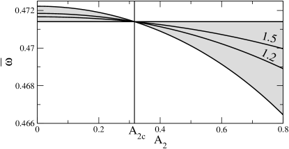
Figure 7: Existence region of nonlinear surface waves (shaded). The curves show the amplitude $A_{2}$ vs. normalized frequency, for different values of the normalized wave number (marked at the curves). All curves intersect at the critical point $A_{2}=A_{2c}$.

Figure 8: Normalized wave number vs. normalized field amplitude $A_{2}$, for different frequencies. Dashed line is $\eta_{2}=0$. The curves on the left of $A_{2c}$ meet the wave number axis at the values corresponding to the linear case. There exist no linear solutions to the right of the critical vertical line $A_{2}=A_{2c}$

The power flow in the linear LH composite medium is given by the result

$$P_{2}=\frac{c^{2}\gamma}{16\pi\omega\mu_{2}\eta_{2}}E_{0}^{2},$$ (27)

and, using the boundary value technique Boardman:1985-1701:JQEL , the power flow in the nonlinear half-space (RH medium) can be obtained in the following form

$$P_{1}=\frac{c^{2}\gamma}{4\pi\omega\mu_{1}^{2}\alpha_{1}}\left(\eta_{1}-\sqrt{\eta_{1}^{2}-E_{0}^{2}\frac{\alpha_{1}\mu_{1}}{2}}\right).$$ (28)

We note here that, although the nonlinear coefficient $\alpha_{1}$ appears as a factor in the denominator of Eq. (28), the reduction to the linear case (when $\alpha_{1}\to 0$) can be performed in a straightforward way by expanding Eq. (28) as for small $\alpha_{1}$ as follows,

$$P_{1}=\frac{c^{2}\gamma}{16\pi\omega\mu_{1}\eta_{1}}E_{0}^{2}+O(\alpha_{1}^{2}),$$ (29)

which has the same form as Eq. (27).

The absolute value of the ratio of the power flow in the RH nonlinear medium to the power flow in the LH composite medium is depicted in Fig. 9. Above the critical value $A_{c}$, there exists a value of the wave number at which the power flow is positive. In this region, there exist a forward travelling surface wave. Note that no matter what the value of the field intensity at the boundary is, there always exists some value of the wave number where the flow is negative and there exists a backward travelling surface wave. This can be seen by reference to Eq. (27). The presence of $\eta_{2}$ in the denominator of Eq. (27) means that as $h$ approaches a value that makes $\eta_{2}=0$ (i.e. a dispersion curve in Fig. 6 approaches the dashed line) the negative power flow in the LH material dominates the total power flow. Conversely, as $\eta_{2}$ increases from zero, the negative power flow in the LH medium decreases so that, provided the intensity of the electric field at the boundary is high enough, the positive power flow in the nonlinear dielectric dominates.

Figure 9: The absolute value of the ratio of the power flow in the nonlinear dielectric to that in the LH material. Above the critical value $A_{c}$, the power flow in the nonlinear half-space dominates giving a forward travelling wave. As $\kappa_{2}$ approaches zero towards the left-hand side of the curves, the power in the left-handed medium dominates.

V Nonlinear pulse propagation and surface-wave solitons

V.1 Envelope equation

Propagation of pulses along the interface between RH and LH media is of a particular interest, since it was shown before Nkoma:1974-3547:JPC for TM modes that the energy fluxes are directed oppositely at either side of the interface. Therefore, we can expect that the energy flow in a pulse with finite temporal and spatial dimension has a nontrivial form Shadrivov:2003-057602:PRE and, in particular, it can be associated with a vortex-like structure of the energy flow.

We analyze the structure of surface waves of both temporal and spatial finite extent that can exist in such a geometry. To obtain the equation describing the pulse propagation along the interface, we look for the structure of a broad electromagnetic pulse with carrier frequency $\omega_{0}$ described by an asymptotic multi-scale expansion with the main terms of the general form

$$\Psi=e^{ih_{0}z-i\omega_{0}t}\left[\Psi_{0}(x)A(\xi,t)-\right.$$

$$\left.i\Psi_{1}(x)\frac{\partial A(\xi,t)}{\partial\xi}+\Psi_{2}(x,\xi,t)+\ldots\right],$$ (30)

where the field $\Psi$ stands for the components $(E_{y},H_{x},H_{z})$ of a TE-polarized wave, the first term $\Psi_{0}=(E_{y0},H_{x0},H_{z0})$ describes the structure of the mode at the carrier frequency $\omega_{0}$, $\Psi_{1}$ is the first-order term of the asymptotic series which can be found as $\Psi_{1}=\partial\Psi_{0}/\partial h$, and $\Psi_{2}$ is the second-order term. Here $A$ is the pulse envelope, $h_{0}$ is the wave number corresponding to the carrier frequency $\omega_{0}$, $\xi=z-v_{g}t$ is the pulse coordinate in the reference frame moving with the group velocity $v_{g}=\partial\omega/\partial h$. Substituting Eq. (V.1) into Eq. (17) and using the Fredholm alternative theorem Korn:MathHandbook , one can obtain the equation for the evolution of the field envelope

$$i\frac{\partial A}{\partial t}+\frac{\delta}{2}\frac{\partial^{2}A}{\partial\xi^{2}}-\omega_{2}(h)|A^{2}|A=0,$$ (31)

where the coefficient $\delta=\partial^{2}\omega/\partial h^{2}$ stands for the group-velocity dispersion (GVD) which determines the pulse broadening and can be calculated from the dispersion relations, $\omega_{2}(h)=\left(\partial\omega_{NL}/\partial A^{2}\right)|_{A=0}$ is the effective nonlinear coefficient calculated with the help of the nonlinear dispersion relation. The NLS equation has a solution in the form of a bright soliton localized at the interface, provided the GVD ($\delta$) has the opposite sign to the sign of the nonlinear coefficient ($\omega_{2}$) (see, e.g., Kivshar:OpticalSolitons and references therein). The existence of the surface polariton solitons has been predicted in a number of structures supporting nonlinear guided waves (see, e.g., Ref. Boardman:1986-8273:PRB and references therein).

The effective nonlinear coefficient for the case of an interface between the nonlinear LH medium and the linear RH medium, can be found using Eq. (III.2),

$$\omega_{2}(h)=-\frac{\alpha\mu_{1}\kappa_{1}\kappa_{2}\omega^{2}}{4hc^{2}(\epsilon_{2}\mu_{2}-\epsilon_{1}\mu_{1})}\frac{d\omega}{dh}.$$ (32)

The signs of the group velocity $d\omega/dh$ and of the parameter $\delta$ can be determined from the Fig. 2. As a result, for any reasonable values of dielectric permittivity and magnetic permeability of the RH medium, there exists a range of frequencies for which $\omega_{2}\cdot\delta<0$, indicating the possibility of exciting surface polariton solitons.

To study the energy flow in such a surface-polariton soliton, we use the asymptotic expansions (V.1) for the field components, and from Eq. (12) we obtain the energy flow structure described by their components

$$S_{z}=\frac{c^{2}h_{0}}{8\pi\omega_{0}\mu}E_{0}^{2}\left|A\right|^{2},$$ (33)

$$S_{x}=\frac{c^{2}}{8\pi\omega_{0}\mu}\left[\frac{\partial E_{0}}{\partial h}\frac{\partial E_{0}}{\partial x}-E_{0}\left(\frac{\partial^{2}E_{0}}{\partial h\partial x}-\frac{v_{gr}}{\omega_{0}}\frac{\partial E_{0}}{\partial x}\right)\right]\cdot$$

$${\rm Re}\left(A\frac{\partial A^{*}}{\partial\xi}\right),$$ (34)

The structure of the Poynting vector in the surface-wave pulse is shown in Fig. (10), where it is clearly seen that the energy rotates in the localized region creating a vortex-type energy distribution in the wave. The difference between the Poynting vector $|S_{z}|$ integrated over the RH medium and that calculated for the LH medium determines the resulting group velocity of the surface wave packet.

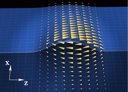
Figure 10: A vortex-like distribution of the Poynting vector in a surface wave soliton propagating along the LH/RH interface.

We note the distinctive vortex-like structure of the surface waves at the interface separating RH and LH media follows as a result of the opposite signs of the dielectric permittivity for the TM-polarized waves and the magnetic permittivity for the TE-polarized waves. These conditions coincide with the conditions for the existence of the corresponding surface waves and, therefore, surface polaritons should always have such a distinctive vortex-like structure.

VI Conclusions

We have presented a systematic study of both linear and nonlinear surface waves supported by an interface between a left-handed metamaterial and a conventional dielectric medium. For the linear regime, we have extended some earlier theoretical results and analyzed different types of surface waves and their existence regions. In particular, we have demonstrated that the structure of the energy flow in a spatially localized wave-packet of the surface waves propagating along the interface has a vortex-like structure. For the case of nonlinear surface waves, we have demonstrated that when only one of the media is nonlinear the maximum amplitude of the spatially localized wave does not shift out the interface. This result is in a sharp contrast to the case of an interface between linear and nonlinear right-handed materials where the maximum of a surface wave is always shifted into a self-focusing nonlinear medium. We have demonstrated that the group velocity of nonlinear surface waves can be controlled by changing the intensity of the electromagnetic field and, in particular, the surface wave can be switched from the forward propagating one to the backward propagating one by varying the field intensity only. In addition, we have obtained the conditions for the existence of the surface-polariton solitons at the metamaterial interface.

References

- (1) V. G. Veselago, Usp. Phys. Nauk 92, 517 (1967).
- (2) D. R. Smith, W. Padilla, D. C. Vier, S. C. Nemat Nasser, and S. Shultz, Phys. Rev. Lett. 84, 4184 (2000).
- (3) L. Venema, Nature 420, 119 (2002).
- (4) J. B. Pendry, Phys. Rev. Lett. 85, 3966 (2000).
- (5) C. Luo, S. G. Johnson, J. D. Joannopoulos, and J. B. Pendry, Phys. Rev. B 65, 201104 (2002).
- (6) R. Ruppin, Phys. Lett. A 277, 61 (2000).
- (7) J. B. Pendry, A. J. Holden, W. J. Stewart, and I. Youngs, Phys. Rev. Lett. 76, 4773 (1996).
- (8) Yu. I. Bespyatyh, A. S. Bugaev, and I. E. Dickshtein, Fizika Tverdogo Tela 43, 2043 (2001).
- (9) F. D. M. Haldane, arXiv:cond-mat/0206420 (2002).
- (10) I. V. Shadrivov, A. A. Sukhorukov, and Yu. S. Kivshar, Phys. Rev. E 67, 057602 (2003).
- (11) R. A. Shelby, D. R. Smith, S. C. Nemat Nasser, and S. Shultz, Appl. Phys. Lett 78, 489 (2001).
- (12) V. A. Podolskiy, A. K. Sarychev, and V. M. Shalaev, Journ. of Nonlin. Opt. Phys. and Materials 11, 65 (2002).
- (13) J. Nkoma, R. Loudon, and D. R. Tilley, J. Phys. C. 7, 3547 (1974).
- (14) Electromagnetic surface modes, A. D. Boardman, ed., (New York : Wiley, 1982).
- (15) A. G. Litvak and V. A. Mironov, Izv. Vuzov: Radiophysica 11, 1911 (1968).
- (16) A. A. Zharov, I. V. Shadrivov, and Yu. S. Kivshar, Phys. Rev. Lett. 91, 037401 (2003).
- (17) V. E. Zakharov and A. B. Shabat, Sov. Phys. JETP 34, 62 (1972).
- (18) A. D. Boardman and P. Egan, IEEE J. Quant. Electron. 21, 1701 (1985).
- (19) A. A. Maradudin, Z-Phys – Condens. Matter 41, 341 (1981).
- (20) G. A. Korn and T. M. Korn, Mathematical Handbook for Scientists and Engineers (McGraw-Hill, New York, 1968).
- (21) Yu. S. Kivshar and G. P. Agraval, Optical solitons. From fibres to photonic crystals (Academic Press, 2003).
- (22) A. D. Boardman, G. S. Cooper, A. A. Maradudin, and T. P. Shen, Phys. Rev. B 34, 8273 (1986).