On stability of renormalized classical electrodynamics

Abstract

It is shown that the total energy of the static “field + particle” system, defined in the framework of classical, renormalized electrodynamics of particles and fields, depends in an unstable way upon the field boundary data. It is argued that this phenomenon may be also an origin of the unstable dynamical behaviour of the system (i.e. existence of “runaway solutions”). It is proved that a suitable polarization mechanism of the particle restores the stability, at least on the level of statics. Whether or not it restores also the full, dynamical stability of the theory is still an open question.

I Introduction

Classical electrodynamics in its present form is unable to describe interaction between charged particles, intermediated by electromagnetic field. Indeed, typical well posed problems of the theory are of the contradictory nature: either we solve partial differential equations for the field, with particle trajectories providing sources (given a priori !), or we solve ordinary differential equations for the trajectories of test particles, with fields providing forces (given a priori !). Combining these two procedures into a single theory leads to a contradiction: Lorentz force due to self-interaction is infinite in case of a point particle.

There were many attempts to overcome these difficulties. One of them consists in using the Lorentz–Dirac equation (see Dirac ,Haag ,Rohr ). Here, an effective force by which the retarded solution computed for a given particle trajectory acts on that particle is postulated (the remaining field is finite and acts by the usual Lorentz force). Unfortunately, this approach leads to the so called runaway solutions which are unphysical.

Various remedies have been proposed to cure such disease, most of them just based on a fine tuning of boundary conditions. Unfortunately, such a tuning excludes physically interesting problems (i.e. circular motion) and the question arises if one can construct a theory which does not contain unphysical solutions at all. The authors believe that to achieve the above goal we should first gain a deeper understanding of foundations of the runaway behaviour.

As a starting point of our analysis, we use an approach proposed by one of us in papers EMP and GKZ . It consists in defining an “already renormalized” four-momentum of the physical system “particle(s) + fields”. Equations of motion are then derived as a consequence of the conservation law imposed on this object. We deeply believe that such an approach is a a correct realization of the Einstein’s programme of “deriving equations of motion from field equations” and that a similar procedure should be applied to formulate the two-body-problem in General Relativity Theory.

We show in the present paper, that the physical instability is inherently contained in the renormalization method used. More precisely: in the simplest renormalization scheme the amount of energy contained “in the interior of the particle” decreases when the external field surrounding the particle increases. This contradicts the stability of the model. As a remedy for such drawback we propose the polarizability of the particle. Numerical analysis of such an improved model shows validity of this proposal.

In this paper we analyze the renormalized energy of the total “particle + field” system on the level of statics only, but the energetic instability discovered this way is obviously a reason for the runaway behaviour of the dynamical system as well. Indeed, the price which must be paid for acceleration becomes negative. This observation is fundamental, in our opinion, to understand the physical reasons for the runaway behaviour of the theory and in search for a remedy for this phenomenon.

The paper is organized as follows. In Section II the renormalization procedure proposed by one of us in EMP (see also GKZ ) is presented. Then a monopole particle inside a fixed volume $V$ is considered: we compute renormalized energy of the system and vary it with respect to particle’s position. Next, we assume that the particle assumes position corresponding to minimal value of the energy. In this way we obtain total energy of the system as a function of the field boundary data, imposed on $\partial V$. Finally, we analyze stability of the system under small changes of these data. Here, both the Dirichlet-type and the Neumann-type boundary problems are considered.

The above general results are then applied to a case of a monopole particle closed in spherical box. We prove that such system is not stable. Then we consider a polarizable particle. Here, the external field may generate a non-vanishing dipole momentum, which changes completely the energy balance. It turns out that for a Heaviside-like relation between the field and the dipole momentum it generates, the system is stable. This suggests a possible way to improve in the future our renormalization method and to avoid (maybe) also dynamical instabilities, manifesting themselves in the runaway behaviour.

II The renormalized four-momentum vector

Full description of the renormalized electrodynamics was proposed in EMP or GKZ . In the present Section we review briefly heuristic ideas that stand behind definition of the renormalized four-momentum of the dynamical “particle + field” system.

As a starting point of our considerations take an extended-particle model. This means that we consider a fully relativistic, gauge-invariant, interacting “matter + electromagnetism” field theory, which is possibly highly non-linear. A moving particle is described by a solution of the theory, such that the “non-linearity-region” (or the “strong-field-region”) is concentrated in a tiny world tube ${\cal W}$ around a smooth, timelike trajectory $\zeta$. We assume that outside of this tube matter fields practically vanish and the electromagnetic field is sufficiently weak to be well described by the linear Maxwell theory. The four momentum of the total system “particle + field” is obtained by integration of a (conserved – due to Noether Theorem) total energy-momentum tensor ${\mathfrak{T}}$:

$${\cal P}_{\lambda}=\int_{\Sigma}{\mathfrak{T}}^{\mu}_{\ \lambda}d\sigma_{\mu}\ ,$$ (1)

over a spacelike hyperplane $\Sigma$.

We assume, moreover, that this fundamental theory admits also a static, stable, soliton-like solution, which will be called a “particle at rest”. Here, the strong-field region (interior of the particle) is assumed to be concentrated around the straight line ${\vec{x}}=$const. Let $m$ denote the total energy (mass) of this solution. Due to relativistic invariance, we have also a six parameter family of solutions obtained by acting with Poincaré transformations on the static solution. Each of these solutions may be called a “uniformly moving particle”. If the solution has been boosted to the four-velocity $u_{\lambda}$ and if $\mathsf{T}(u)$ denotes its energy-momentum tensor, then the total four-momentum of this solution equals $mu_{\lambda}$ and we have:

$$mu_{\lambda}=\int_{\Sigma}\mathsf{T}^{\mu}_{\ \lambda}(u)d\sigma_{\mu}\ .$$ (2)

This leads to a trivial identity:

$${\cal P}_{\lambda}=mu_{\lambda}+\int_{\Sigma}\left({\mathfrak{T}}^{\mu}_{\ \lambda}-\mathsf{T}^{\mu}_{\ \lambda}(u)\right)d\sigma_{\mu}\ ,$$ (3)

which becomes extremely useful in the following arrangement. We assume that the straight line which describes the “trajectory” of the second (uniformly moving) particle is tangent to the approximate trajectory $\zeta$ of the first (i.e. generic) particle at their intersection point with $\Sigma$. If $K(R)\subset\Sigma$ denotes the ball of radius $R$, which contains the strong field region of both solutions, but is small with respect to the characteristic distance of the external Maxwell fields, then we have:

$${\cal P}_{\lambda} = mu_{\lambda}+\int_{\Sigma-K(R)}\left({\mathfrak{T}}^{\mu}_{\ \lambda}-\mathsf{T}^{\mu}_{\ \lambda}(u)\right)d\sigma_{\mu}+$$ (4)

$$+ \int_{K(R)}\left({\mathfrak{T}}^{\mu}_{\ \lambda}-\mathsf{T}^{\mu}_{\ \lambda}(u)\right)d\sigma_{\mu}\ .$$

Our assumption about stability of the free particle (soliton solution) means that the last integral is negligible since inside the particle both solutions are very close to each other. But the first integral contains only contributions from external Maxwell fields accompanying both particles. This way we have proved that the following formula:

$${\cal P}_{\lambda}\simeq mu_{\lambda}+\int_{\Sigma-K(R)}\left({\mathfrak{T}}^{\mu}_{\ \lambda}-\mathsf{T}^{\mu}_{\ \lambda}(u)\right)d\sigma_{\mu}\ ,$$ (5)

containing only external Maxwell field surrounding the particle, provides a good approximation of the total four-momentum of the total “particle + field” system.

The theory proposed in EMP consists in mimicking the above formula in the point particle model. Hence, we consider solutions of Maxwell equations having a “delta-like” current corresponding to a point charge $e$ traveling over a trajectory $\zeta$. Such a solution is treated as an idealized description of external properties of the extended particle considered above. Denote by $T$ the energy momentum tensor of this solution. Of course, the uniformly moving particle, whose four-velocity equals $u$, is represented in this picture by a boosted Coulomb field, and its energy-momentum tensor is denoted by $\mathbb{T}(u)$. If trajectories of both particles are again tangent with each other at their common point of intersection with $\Sigma$, then momentum (5) may be rewritten as:

$${\cal P}_{\lambda}\simeq mu_{\lambda}+\int_{\Sigma-K(R)}\left({T}^{\mu}_{\ \lambda}-\mathbb{T}^{\mu}_{\ \lambda}(u)\right)d\sigma_{\mu}\ ,$$ (6)

because outside of the particle ${\mathfrak{T}}$ reduces to $T$ and $\mathsf{T}(u)$ reduces to $\mathbb{T}(u)$. The main observation done in EMP is that, due to cancellation of principal singularities of both $T$ and $\mathbb{T}$(u), the above integration may be extended to the entire $\Sigma$. More precisely, the following quantity:

$${\cal P}_{\lambda}:=mu_{\lambda}+P\int_{\Sigma}\left(T^{\mu}_{\ \lambda}-\mathbb{T}^{\mu}_{\ \lambda}(u)\right)d\sigma_{\mu}\ ,$$ (7)

is well defined (“$P$” denotes the “principal value” of the integral). According to the discussion above, we interpret this quantity as the total four-momentum of the interacting system composed of the point particle and the Maxwell field accompanying the particle. Consequently, we impose conservation of ${\cal P}$ as an additional condition. This implies equations of motion of the point particle as a good approximation of equations of motion of the true, extended particle.

This approach has an obvious generalization to the system of many particles (see EMP ). Also polarizable particles, carrying magnetic or electric moment (and – consequently – displaying stronger field singularity than the Coulomb field) may be treated this way (cf. praca-dokt ). Recently, the above approach was improved by replacing the reference Coulomb field in (7) by the Born field, matching not only particle’s velocity but also its acceleration. This way the principal-value-sign “$P$” may be omitted in the definition because the corresponding integral converges absolutely (cf. KP ).

In what follows, we are going to apply definition (7) to static “particle + field” configurations only.

III Electrostatics of a monopole particle

Consider now electrostatic field $D$ surrounding the particle with charge $e$, situated at the point $\vec{r}_{0}$. Due to Maxwell equations, the Gauss law:

$$\nabla{D}=e{\boldsymbol{\delta}}\left(\vec{r}-\vec{r}_{0}\right)\ ,$$ (8)

must be satisfied, where by ${\boldsymbol{\delta}}$ we denote Dirac delta distribution (in contrast with conventional $\delta$, denoting variation of a function). It is, therefore, convenient to decompose the field into its singular and regular parts:

$$D=D_{reg}+D_{sing},$$ (9)

where the singular part $D_{sing}$ is simply the Coulomb field:

$$D_{sing}:=\frac{e\left(\vec{r}-\vec{r}_{0}\right)}{4\pi\|\vec{r}-\vec{r}_{0}\|^{3}}\ ,$$

whereas the remaining field $D_{reg}:=D-D_{sing}$ is divergenceless: $\nabla D_{reg}=0$. Moreover, static Maxwell equations imply the existence of the scalar potential $\phi$: $D=-\nabla\phi$. Hence, we have: $\Delta\phi_{reg}=0$.

According to (7), the complete energy of this “particle + field” system contained in the the entire $\Sigma$ equals:

$${\cal H}=m+\frac{1}{2}\int_{\Sigma}\left({D}^{2}-D_{sing}^{2}\right)dv\ .$$ (10)

We suppose that the particle is contained in a fixed volume $V\ni\vec{r}_{0}$. Subtracting from ${\cal H}$ the electrostatic energy contained outside of $V$:

$${\cal H}_{{\mathbb{R}^{3}}-V}=\frac{1}{2}\int_{{\mathbb{R}^{3}}-V}{D}^{2}dv\ ,$$ (11)

we obtain the total energy contained in $V$:

$${\cal H}_{V} = m-\frac{1}{2}\int_{{\mathbb{R}^{3}}-V}{D_{sing}}^{2}dv+\frac{1}{2}\int_{V}{D_{reg}}^{2}dv+$$ (12)

$$+ \int_{V}D_{sing}D_{reg}dv.$$

Given boundary conditions, we are going to minimize the above quantity with respect to the particle’s position $\vec{r}_{0}\in V$. Assuming that the particle always tries to minimize the energy of the system, we can write both $\vec{r}_{0}$ and the total “particle+field” energy as functions of the field boundary data. Stability of the energy with respect to the boundary data on $\partial V$ will then be studied. Before we pass to the above programme, we must specify which kind of boundary conditions on $\partial V$ have to be controlled.

III.1 Neumann conditions

Varying the energy integral (12) with respect to the particle’s position we get:

$$\delta{\cal H}_{V}= \int_{V}\left\{D_{reg}\cdot\left(\delta D_{reg}+\delta D_{sing}\right)+D_{sing}\,\delta D_{reg}\right\}dv$$

$$-\int_{{\mathbb{R}}^{3}-V}D_{sing}\,\delta D_{reg}\,dv.$$ (13)

For Neumann conditions we put $D=-\nabla\phi$ for both the regular and the singular parts of the field, outside of the variation $\delta$. Integrating by parts and using $\nabla D_{reg}=0$ we get:

$$\delta{\cal H}_{V}=\int_{V}\phi_{reg}\,\delta(\nabla D_{sing})dv-\int_{\partial V}\left\{\phi\,\delta D^{\bot}\right\}\,d\sigma.$$ (14)

But the variation of (8) gives us:

$$\delta(\nabla D_{sing})=\delta\left(e{\boldsymbol{\delta}}\left(\vec{r}-\vec{r}_{0}\right)\right)=-e\partial_{k}\left({\boldsymbol{\delta}}\left(\vec{r}-\vec{r}_{0}\right)\right)\delta x_{0}^{k},$$ (15)

where $\delta x_{0}^{k}$ denotes a virtual displacement of the particle. Imposing Neumann conditions $D^{\bot}|\partial V=f$, where $f$ is a fixed function, we obtain: $\delta D^{\bot}\equiv 0$ on $\partial V$. Hence, the surface integral vanishes. Inserting (15) into (14) we derive the following formula:

$$\delta{\cal H}_{V}=-eD^{\text{reg}}_{k}(x^{k}_{0})\delta x^{k}_{0}.$$ (16)

We conclude that the extremum of energy condition implies the following static equilibrium equation:

$$D^{\text{reg}}_{k}(x^{k}_{0})=0\ .$$ (17)

III.2 Dirichlet conditions

For Dirichlet case we put $\delta D=-\nabla\delta\phi$ for both the regular and the singular parts of the field and then integrate (III.1) by parts. We obtain:

$$\delta{\cal H}_{V}=\int_{V}\left(\nabla D_{sing}\right)\delta\phi_{reg}dv-\int_{\partial V}\left\{D^{\bot}\,\delta\phi\right\}\,d\sigma.$$ (18)

Imposing Dirichlet conditions $\phi|\partial V=f$, where $f$ is a fixed function, we obtain: $\delta\phi\equiv 0$ on $\partial V$ and, therefore, the surface integral vanishes again. To derive the equilibrium condition (17) from the variational principle, we must perform the following Legendre transformation:

$$\int_{V}\left(\nabla D_{sing}\right)\delta\phi_{reg}dv =\delta\int_{V}\left(\nabla D_{sing}\right)\phi_{reg}dv+$$

$$-\int_{V}\left(\delta\nabla D_{sing}\right)\phi_{reg}dv\ .$$ (19)

Then we use (8) and (15). This way we obtain:

$$\delta\left({\cal H}_{V}-e\phi_{reg}({\vec{r}}_{0})\right)=D^{\text{reg}}_{k}(x^{k}_{0})\delta x^{k}_{0}.$$ (20)

Comparing (16) and (20) we observe that the equilibrium condition (17) may either be obtained from the variational principle $\delta\left({\cal H}_{V}\right)=0$, when the Neumann boundary data are controlled, or from the variational principle $\delta\left({\cal F}_{V}\right)=0$, with ${\cal F}_{V}:={\cal H}_{V}-e\phi_{reg}({\vec{r}}_{0})$, when the Dirichlet boundary data are controlled. The quantity ${\cal H}_{V}$ is the total energy of the “particle + field” system, whereas ${\cal F}_{V}$ is an analog of the free energy in thermodynamics. We conclude that imposing Neumann condition on the boundary corresponds to the adiabatic insulation of the system, whereas imposing Dirichlet condition means that we expose it to a kind of a “thermal bath”. Indeed, imposing e.g. condition $\phi|\partial V=0$ we must cover the surface $\partial V$ with a metal shell and ground it electrically. This means that we admit energy exchange of our system with the earth. Similarly as in thermodynamics, the free energy ${\cal F}_{V}$, which we optimize, contains not only the system’s energy ${\cal H}_{V}$ but also the term “$-e\phi_{reg}({\vec{r}}_{0})$” which we interpret as energy of the “boundary-condition-controlling device”. Of course, from the point of view of the particle, both conditions lead to the same equation: $D^{\text{reg}}(x^{k}_{0})=0$ because our theory is local and the particle interacts with its immediate neighbourhood only, no matter how the boundary data are controlled far away from the particle.

IV An example – monopole particle in a spherical box

In this section we shall analyze stability of a charged, monopole particle closed in a spherical box with radius $R$: $V=K(0,R)\subset{\mathbb{R}}^{3}$. Simplicity of the model allows us to solve explicitly the static Maxwell equations (for both the Neumann and the Dirichlet cases) and to compute renormalized energy of the system. Then we will find the extremum of the energy function with respect to the particle’s position and check that for the Neumann case we get the minimum and for the Dirichlet case – the maximum of the energy. Assuming that the particle always minimizes the energy, we will express energy function in terms of the boundary data and show that the system is unstable under small changes of these data.

The problem consists in solving equation $\Delta\phi=-e\delta(\vec{r}-\vec{r}_{0})$, where $\vec{r}_{0}\in K(0,R)$. In the Neumann case we impose the following condition:

$$\vec{D}\cdot\vec{n}{\big{|}}_{r=R}=\vec{E}\cdot\vec{n}+\frac{e}{4\pi R^{2}}\ ,$$ (21)

where $\vec{E}$ is a fixed three dimensional vector.

In the Dirichlet case we impose the following condition:

$$\phi{\big{|}}_{r=R}=-\vec{E}\cdot\vec{n}\,R+\frac{e}{4\pi R}\ .$$ (22)

Because of the axial symmetry of the problem, we may restrict ourselves to the analysis of the energy functional at points $\vec{r}_{0}$ which are parallel to $\vec{E}$: $\vec{r}_{0}\|\vec{E}$. With this simplification, we are able to find an explicit solution $\phi=\phi_{sing}+\phi_{reg}$, where:

$$\phi_{sing}=\frac{1}{4\pi}\frac{e}{|\vec{r}-\vec{r_{0}}|}\ ,$$

in both Dirichlet and Neumann cases (cf. Appendices A and C). To write an explicit formula for $\phi_{reg}$ it is useful to introduce the following variable:

$$r_{0}:=\frac{1}{\|E\|}(\vec{E}|\vec{r}_{0})\ ,$$

which runs from $-R$ to $R$. Under this convention we obtain:

$$\phi_{reg}=\frac{e}{4\pi}\bigg{(}\frac{R}{\sqrt{R^{4}+{r_{0}}^{2}r^{2}-2r_{0}rR^{2}\cos\theta}}-\frac{1}{R}+$$

$$-\frac{1}{R}\ln\left|R^{2}-r_{0}r\cos\theta+\sqrt{R^{4}+{r_{0}}^{2}r^{2}-2r_{0}rR^{2}\cos\theta}\right|\bigg{)}$$

$$-\vec{E}{\vec{r}}+\frac{1}{R}\ln(2R^{2})\ ,$$ (23)

in the Neumann case, whereas:

$$\phi_{reg} =\frac{e}{4\pi}\bigg{(}\frac{1}{R}-\frac{R}{\sqrt{R^{4}+{r_{0}}^{2}r^{2}-2r_{0}rR^{2}\cos\theta}}\bigg{)}-\vec{E}{\vec{r}}\ ,$$ (24)

in the Dirichlet case.

IV.1 Stability

In both cases, the renormalized energy can be computed explicitly. Denoting $E:=\|\vec{E}\|$ we obtain the following result:

$${\cal H}_{\cal N}= m+\frac{1}{2}\left(\frac{e^{2}}{4\pi}\left(\frac{R}{R^{2}-r_{0}^{2}}-\frac{1}{R}\ln\left|1-\frac{r_{0}^{2}}{R^{2}}\right|-\frac{2}{R}\right)+\right.$$

$$\left.+\frac{4}{3}\pi R^{3}E^{2}-2eEr_{0}\right),$$ (25)

in the Neumann case (cf. Appendix B) and:

$${\cal H}_{\cal D}=m+\frac{1}{2}\left(\frac{4}{3}\pi R^{3}E^{2}-\frac{e^{2}}{4\pi}\frac{R}{R^{2}-r_{0}^{2}}\right)\ ,$$ (26)

in the Dirichlet case (cf. Appendix C). Finally, we compute the electric “free energy” ${\cal F}={\cal H}-e\phi_{reg}(\vec{r}_{0})$ in the Dirichlet case:

$${\cal F}=m+\frac{1}{2}\left(\frac{e^{2}}{4\pi}\frac{R}{R^{2}-r_{0}^{2}}+2eEr_{0}+\frac{4}{3}\pi R^{3}E^{2}-\frac{e^{2}}{4\pi}\frac{2}{R}\right).$$ (27)

We see that the equilibrium condition in the Neumann case reads:

$$D_{reg}{\big{|}}_{\vec{r}=\vec{r}_{0}}=0\Leftrightarrow\left(eE-\frac{e^{2}}{4\pi}\frac{r_{0}}{R(R^{2}-r_{0}^{2})}\right)=0\ ,$$ (28)

whereas in the Dirichlet case it reads:

$$eD_{reg}{\big{|}}_{\vec{r}=\vec{r}_{0}}=\frac{e^{2}}{4\pi}\frac{Rr_{0}}{(R^{2}-r_{0}^{2})^{2}}+eE=\frac{\partial}{\partial r_{0}}{\cal F}\ .$$ (29)

We express the energy in terms of the following, standardized variables:

$$x=\frac{r_{0}}{R}\in]-1,1[,\qquad q=\frac{4\pi R^{2}}{e}E\ .$$ (30)

Denoting:

$${\cal H^{\prime}}=({\cal H}-m)\frac{8\pi R}{e^{2}}\ ,$$ (31)

we obtain:

$${\cal{H^{\prime}}_{N}} =\frac{1}{1-x^{2}}-\ln|1-x^{2}|-2qx+\frac{1}{3}q^{2}-2,$$ (32)

$${\cal{H^{\prime}}_{D}} =\frac{1}{3}q^{2}-\frac{1}{1-x^{2}}.$$ (33)

Observe that for $q=0$ both energies may be expanded as follows (cf. figure 1):

$${\cal{H^{\prime}}_{N}} = -1+2x^{2}+O(x^{4})\ ,$$ (34)

$${\cal{H^{\prime}}_{D}} = -1-x^{2}+O(x^{4})\ .$$ (35)

This implies that only in the Neumann case the equilibrium point ($x=0$) is also a minimum of the energy. In the Dirichlet case the energy has a local maximum at the equilibrium point. As may be easily seen, this happens also for any value of $E$. Hence, for the Dirichlet case the free energy $\cal F$ should be used, for which local extremum is also minimum. In what follows we shall use the local, physical energy and consequently, we restrict ourselves to the Neumann case only.

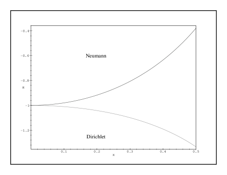
Figure 1: Graph of renormalized energy vs particle’s position and $q=0$ for ${\cal{H^{\prime}}_{N}}$ and ${\cal{H^{\prime}}_{D}}$

IV.2 Neumann conditions

In terms of the standardized variables, the equilibrium condition (28) reads:

$$q=\frac{x(2-x^{2})}{(1-x^{2})^{2}}\ .$$ (36)

For small values of $q$ this enables us to express equilibrium position in terms of the boundary data:

$$x\approx\frac{q}{2}\ .$$ (37)

The same result could be obtained from the following expansion:

$${\cal{H^{\prime}}_{N}}(x,q)=-1+\frac{1}{3}q^{2}-2qx+2x^{2}+O(x^{4}),$$ (38)

$$\partial_{x}{\cal{H^{\prime}}_{N}}(x,q)=0\Rightarrow x\approx\frac{q}{2},$$ (39)

$${\cal{H^{\prime}}_{N}}(x,q){|}_{x=\frac{q}{2}}=-1-\frac{1}{6}q^{2}+O(q^{3}).$$ (40)

Observe that for increasing values of $q$, the energy of the system decreases (cf. figure 2)! The system “particle + field” turns out to be unstable – even small fluctuations of the external field $q$ can decrease its total energy. This means that the particle behaves like a perpetuum mobile, providing a source of energy at no costs. In our opinion this unphysical feature of the model, manifestly seen in its static behaviour, could possibly be a source of its dynamical instability, i.e. the existence of “runaway” solutions of Dirac equation. As a remedy, described in the sequel, we propose to equip the particle with an additional mechanism which, via electric polarizability, will restore its static stability.

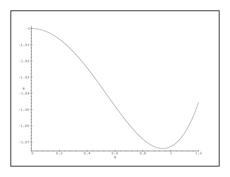
Figure 2: Graph of renormalized energy vs boundary field $q$ for ${\cal{H^{\prime}}_{N}}(x(q),q)$

V Polarizable particle

We assume that the particle may get a non-vanishing electric dipole moment due to interaction with the neighboring field. We prove in the sequel that, under a suitable choice of the polarizability properties of the particle, the resulting “particle + field” system becomes statically stable.

For a polarized particle, formula (12) for the total energy remains valid but the field singularity is now deeper than in (8), namely:

$$\nabla D=\nabla D_{sing}=e{\boldsymbol{\delta}}(\vec{r}-\vec{r}_{0})-p^{k}\partial_{k}{\boldsymbol{\delta}}(\vec{r}-\vec{r}_{0})\ ,$$ (41)

where $p^{k}$ is a dipole moment. We assume that $p^{k}$ has been generated by the surrounding electric field $D$ according to some law $p=p(D_{reg}(\vec{r}_{0}))$, describing the sensitivity of the particle. Moreover, we admit the dependence of the coefficient $m$ in (7) (and, consequently, in (12)) upon polarization. It will be shown in the sequel that insisting in having $m$ constant we are not able to make the model physically consistent. Moreover, it will be shown that the electric sensitivity is uniquely implied by the dependence $m=m(p)$.

V.1 Variational principle

Variation of the renormalized energy (12) with respect to the particle’s position contains now the non-vanishing term $\delta m$. Similar calculations as for the scalar particle lead, in case of the Neumann boundary conditions, to formula:

$$\delta{\cal H}_{V} = \delta m+\int_{V}\phi_{reg}\delta(\nabla D_{sing})dv+$$ (42)

$$- \int_{\partial V}\left\{\phi\,\delta D^{\perp}\right\}\,d\sigma\ ,$$

and, in case of the Dirichlet conditions, to:

$$\delta{\cal H}_{V}=\delta m+\int_{V}(\nabla D_{sing})\delta\phi_{reg}dv-\int_{\partial V}\left\{D^{\perp}\delta\phi\right\}\,d\sigma=$$

$$\delta m+\delta\int_{V}(\nabla D_{sing})\phi_{reg}dv-\int_{V}\phi_{reg}\delta(\nabla D_{sing})dv+$$

$$-\int_{\partial V}\left\{D^{\perp}\delta\phi\right\}\,d\sigma\ .$$ (43)

According to (41), the new version of formula (15) reads:

$$\delta(\nabla D_{sing}) =-\left(e\partial_{k}{\boldsymbol{\delta}}(\vec{r}-\vec{r}_{0})-p^{j}\partial_{j}\partial_{k}{\boldsymbol{\delta}}(\vec{r}-\vec{r}_{0})\right)\delta x^{k}_{0}+$$

$$-\left(\partial_{k}{\boldsymbol{\delta}}(\vec{r}-\vec{r}_{0})\right)\delta p^{k}\ .$$ (44)

Plugging (V.1) into (42) we see that the total energy variation splits into the sum of two pieces: the work due to virtual displacement of the particle and the remaining work, due to variation of $m$ and $p$:

$$\delta{\cal H}_{V} =\underbrace{-\left(eD_{reg}+p^{k}\partial_{k}D_{reg}\right){\big{|}}_{\vec{r}=\vec{r}_{0}}}_{{\cal A}}\delta\vec{r}_{0}+$$

$$+\underbrace{\delta m-D_{reg}{\big{|}}_{\vec{r}=\vec{r}_{0}}\delta p}_{{\cal B}}\ .$$ (45)

The second part $\cal B$ is obviously nonlocal – both the mass $m$ and the moment $p$ depend upon the value of $D_{reg}(\vec{r}_{0})$. This quantity must be obtained from the field equation: $\Delta\phi_{reg}=0$, with boundary value depending upon the particle’s position. The only way to save locality of the model is to force the term $\cal B$ to vanish identically by imposing the following constraint:

$$\delta m=D_{reg}(\vec{r}_{0})\delta p\ .$$ (46)

Denoting by $m_{0}=m(0)$ the mass of the unpolarized particle and by $f(p)$ the additional polarization energy:

$$m(p)=m_{0}+f(p)\ ,$$ (47)

formula (46) may be written as:

$$D^{reg}_{k}(\vec{r}_{0})=\frac{\partial f(p)}{\partial p^{k}}\ .$$ (48)

We see that the polarization energy $f$ must play role of the generating function for the polarizability relation, otherwise the model would not be local. Indeed, suppose that ${\cal B}$ does not vanish and the particle’s equilibrium condition needs vanishing of the whole right hand side of (V.1). To decide whether or not its actual position is acceptable as an equilibrium position, the particle must know not only the field in its immediate neighbourhood, but also the shape of $V$ and the field boundary data on $\partial V$. Such a behaviour is physically non acceptable.

Inverting the generating formula (48), we may find the dependence $p=p(D_{reg}(\vec{r}_{0}))$, which is uniquely implied by the “equation of state” (47). Hence, we have:

$$\delta{\cal H}_{V}=-\left(eD_{reg}+p^{k}\partial_{k}D_{reg}\right){\big{|}}_{\vec{r}=\vec{r}_{0}}\delta\vec{r}_{0}\ ,$$ (49)

and the equilibrium condition becomes a local equations:

$$\left(eD_{reg}+p^{k}\partial_{k}D_{reg}\right){\big{|}}_{\vec{r}=\vec{r}_{0}}=0\ .$$ (50)

A similar procedure works in the Dirichlet case as well. Applying the state equation to (43) we obtain:

$$\delta{\cal F}_{V}=\left(eD_{reg}+p^{k}\partial_{k}D_{reg}\right){\big{|}}_{\vec{r}=\vec{r}_{0}}\delta\vec{r}_{0}\ ,$$ (51)

where the “free energy” ${\cal F}_{V}$ is given as:

$${\cal F}_{V}:={\cal H}_{V}-\int_{V}(\nabla D_{sing})\phi_{reg}-2f$$

$$:={\cal H}_{V}-e\phi_{reg}(\vec{r}_{0})+D_{reg}{\big{|}}_{\vec{r}=\vec{r}_{0}}\cdot p-2f\ .$$ (52)

Equilibrium condition $\delta{\cal F}_{V}=0$ reduces to the same, local equation (50).

VI An example – polarizable particle in a spherical box

Let us come back to the simple model described in Section IV on page IV. For the polarizable particle we must solve the field equation:

$$\Delta\phi=-e\delta(\vec{r}-\vec{r}_{0})+\vec{p}\cdot\nabla(\delta(\vec{r}-\vec{r}_{0}))\ ,$$ (53)

where $\vec{r}_{0}\in K(0,R)$, with either Neumann (21) or Dirichlet condition (22). We want to compute renormalized total energy of the “particle + field” system and to prove that for a suitable state equation (47) our model becomes stable.

Splitting the solution $\phi$ into two parts:

$$\phi=\phi^{mon}+\phi^{dip}\ ,$$ (54)

where by $\phi^{mon}$ we denote the solution of the monopole problem, found earlier (cf. Section (IV), page 23), we reduce the problem to equation:

$$\Delta\phi^{dip}=\vec{p}\cdot\nabla\,(\delta(\vec{r}-\vec{r}_{0}))\ ,$$ (55)

with homogeneous boundary conditions: $\vec{D}^{dip}\cdot\vec{n}{\big{|}}_{r=R}=0$ in the Neumann case and $\phi^{dip}{\big{|}}_{r=R}=0$ in the Dirichlet case. Choosing the axis ${\boldsymbol{e}_{z}}$ parallel to $\vec{E}$ and passing to spherical coordinates $(r,\theta,\varphi)$ we obtain for $\vec{r}_{0}=(r_{0},0,0)$ and $\vec{p}=p{\boldsymbol{e}_{z}}+p_{x}{\boldsymbol{e}_{x}}$ (see Appendix D on page D):

$$\phi^{dip}=\phi^{dip}_{sing}+\phi^{dip}_{reg}\ ,$$ (56)

where:

$$\phi^{dip}_{sing}=\frac{1}{4\pi}\frac{\vec{p}\cdot(\vec{r}-\vec{r}_{0})}{|\vec{r}-\vec{r}_{0}|^{3}},$$ (57)

$$\phi^{dip}_{reg}=\frac{p}{4\pi}\left(\frac{R^{3}\left(R^{2}-rr_{0}\cos\theta\right)}{r_{0}\left(R^{4}+(r_{0}r)^{2}-2rr_{0}R^{2}\cos\theta\right)^{\frac{3}{2}}}-\frac{1}{r_{0}R}\right)$$

$$+\frac{p_{x}}{4\pi}\Bigg{(}\frac{rR^{3}\sin\theta\cos\varphi}{(R^{4}+{r_{0}}^{2}r^{2}-2r_{0}rR^{2}\cos\theta)^{\frac{3}{2}}}+$$

$$-\frac{\cos\varphi(R^{2}\cos\theta-r_{0}r)}{Rr_{0}\sin\theta\sqrt{R^{4}+{r_{0}}^{2}r^{2}-2r_{0}rR^{2}\cos\theta}}+\frac{\cos\theta\cos\varphi}{Rr_{0}\sin\theta}\Bigg{)}.$$ (58)

As we already noticed in the monopole case, axial symmetry of the problem implies that minimum of the energy is assumed at the point $\vec{r}_{0}$ which is parallel to $\vec{E}$. The same argument implies that we have ${p_{x}}=0$ in this configuration. We are going to limit our analysis to such configurations only.

VI.1 Stability

We compute the total, renormalized energy of the system as a sum of two parts:

$${\cal H}={\cal H}^{mon}+{\cal H}^{dip}\ ,$$ (59)

where ${\cal H}^{mon}$ denotes the energy of the monopole field obtained earlier ((IV.1), page IV.1), and ${\cal H}^{dip}$ denotes the remaining part, containing energy of the dipole field and the interaction energy. The latter term is computed in Appendix E (page E). The final result for the Neumann case, written in terms of standardized variables reads:

$${\cal H_{N}}^{\prime}(x,q,p)=\frac{1}{1-x^{2}}-\ln|1-x^{2}|-2qx+\frac{1}{3}q^{2}-2+$$

$$+\frac{2}{3}\left(\frac{p}{eR}\frac{x(2-x^{2})}{(1-x^{2})^{2}}-\frac{p^{2}}{e^{2}R^{2}}\frac{1}{(1-x^{2})^{3}}-\frac{p}{eR}\,q\right).$$ (60)

Now, stability of the system depends upon the polarizability of the particle, i.e. upon the choice of the “state function” $f$ (cf. (47) on page 47). At the moment we have no general criterion which would guarantee stability. However, it is easy to show that for:

$$f(\vec{p})=-\frac{c^{2}}{3}\|\vec{p}\|^{3}\Longrightarrow D_{reg}=-c^{2}\|\vec{p}\|\vec{p},\quad c>0\ ,$$ (61)

our system is stable. Indeed, using (23) and (58) we obtain the following equation for the value of the dipole moment $p$:

$$-c^{2}p^{2}\mbox{\rm sgn}(p)=D_{reg}{\bigg{|}}_{\vec{r}=\vec{r}_{0}}=-\nabla\left({\phi}^{mon}_{reg}+{\phi}^{dip}_{reg}\right)=$$

$$=\frac{1}{4\pi}\left(\frac{eq}{R^{2}}-\frac{2p}{R^{3}(1-x^{2})^{3}}-\frac{ex(2-x^{2})}{R^{2}(1-x^{2})^{2}}\right)\ .$$ (62)

Denoting $4\pi ec^{2}R^{4}=C$ and ${\widetilde{p}}=\frac{p}{eR}$, we get equation for $\widetilde{p}$:

$$-C{\widetilde{p}}^{2}\mbox{\rm sgn}({\widetilde{p}})=\left(q-\frac{2{\widetilde{p}}}{(1-x^{2})^{3}}-\frac{x(2-x^{2})}{(1-x^{2})^{2}}\right)\ .$$ (63)

For small $x$, we use Taylor expansion of the right hand side. Consequently, we have:

$$-C{\widetilde{p}}^{2}\mbox{\rm sgn}({\widetilde{p}})\approx q-2{\widetilde{p}}-2x-6{\widetilde{p}}x^{2}-3x^{3}.$$ (64)

For ${\widetilde{p}}>0$ there are two solutions of this equation for small $x$ and $q$:

$${\widetilde{p}}_{1} \approx \frac{1}{C}\left(1+\sqrt{1-qC}+\frac{xC}{\sqrt{1-qC}}\right)\ ,$$ (65)

$${\widetilde{p}}_{2} \approx \frac{1}{C}\left(1-\sqrt{1-qC}-\frac{xC}{\sqrt{1-qC}}\right)\ .$$ (66)

For ${\widetilde{p}}<0$ there is only one solution for small $x$ and $q$:

$${\widetilde{p}}_{3}\approx-\frac{1}{C}\left(1+\sqrt{1+qC}-\frac{xC}{\sqrt{1+qC}}\right).$$ (67)

Inserting the above solutions into the energy function (VI.1) we define for $i=1,2,3$:

$${\cal H^{\prime}}_{i}(x,q)={\cal H_{N}}^{\prime}(x,q,eR{\widetilde{p}}_{i})\ .$$

It turns out that ${\cal H^{\prime}}_{2}$ does not admit any minimum with respect to $x$ (i.e. a stable “field + particle” configuration). For the remaining two cases we use Taylor expansion for small $x$:

$${\cal H^{\prime}}_{1}\approx-1+\frac{1}{3}q^{2}-\frac{4}{3C^{2}}+\frac{2}{3\sqrt{1-qC}}\left(-\frac{2}{C^{2}}+\frac{q}{C}+q^{2}\right)$$

$$-2q\left(1+\frac{1}{\sqrt{1-qC}}\right)x+2\left(1-\frac{2}{C^{2}}+\frac{q}{C}-\frac{1}{3}\frac{1}{1-qC}\right.$$

$$\left.+\frac{2}{\sqrt{1-qC}}\left(\frac{1}{3}-\frac{1}{C^{2}}+\frac{q}{C}\right)\right)x^{2}.$$ (68)

$${\cal H^{\prime}}_{3}\approx-1+\frac{1}{3}q^{2}-\frac{4}{3C^{2}}+\frac{2}{3\sqrt{1+qC}}\left(-\frac{2}{C^{2}}-\frac{q}{C}+q^{2}\right)$$

$$-2q\left(1+\frac{1}{\sqrt{1+qC}}\right)x+2\left(1-\frac{2}{C^{2}}-\frac{q}{C}-\frac{1}{3}\frac{1}{1+qC}\right.$$

$$\left.+\frac{2}{\sqrt{1+qC}}\left(\frac{1}{3}-\frac{1}{C^{2}}-\frac{q}{C}\right)\right)x^{2}$$ (69)

Minimizing both energies with respect to $x$ we obtain:

$$x_{1}(q)\approx \frac{3C^{2}}{32(C^{2}-3)}\left(8q+\frac{2C(C^{2}-9)}{C^{2}-3}q^{2}+\right.$$

$$+ \left.\frac{C^{2}(2C^{4}-15C^{2}+45)}{(C^{2}-3)^{2}}q^{3}\right),$$ (71)

$$x_{3}(q)\approx \frac{3C^{2}}{32(C^{2}-3)}\left(8q-\frac{2C(C^{2}-9)}{C^{2}-3}q^{2}+\right.$$

$$+\left.\frac{C^{2}(2C^{4}-15C^{2}+45)}{(C^{2}-3)^{2}}q^{3}\right).$$ (72)

Plugging $x_{i}(q)$ into the energy we get for small $q$:

$${\cal H^{\prime}}_{1}(q) \approx-1-\frac{8}{3C^{2}}+\frac{15+4C^{2}}{6(3-C^{2})}q^{2}+$$

$$+\frac{(18+42C^{2}-7C^{4})C}{12(3-C^{2})^{2}}q^{3},$$ (73)

$${\cal H^{\prime}}_{3}(q) \approx-1-\frac{8}{3C^{2}}+\frac{15+4C^{2}}{6(3-C^{2})}q^{2}+$$

$$-\frac{(18+42C^{2}-7C^{4})C}{12(3-C^{2})^{2}}q^{3}.$$ (74)

We see that for $C\in]0,\sqrt{3}[$ the $q^{2}$ term is positive. This means that the system “particle + field” does not behave any longer like a perpetuum mobile: to deform its original configuration, corresponding to $q=0$, the boundary-condition controlling device must perform a positive work. Hence, the system is stable under small changes of $q$ (see figure 3).

Figure 3: Graph of ${\cal H^{\prime}}(q)$ – renormalized energy vs boundary field for dipole particle, $C=1$

VI.2 Conclusions

We have shown that the polarizability of the particle, described by a suitable “state function” $f$ (e.g. by (61)), may be a good remedy for the static instability of the renormalized electrodynamics of point particles. Whether or not this will cure also the dynamical instability, i.e. the existence of “runaway” solutions, is another question which we would like to study in the nearest future.

At the moment the bifurcation phenomenon occurring near the ground state $q=0$ is worthwhile to study. Observe that the point $\vec{r}_{0}=0$, corresponding to $q=0$ and described by the purely monopole field, is not stable. This configuration corresponds to a local maximum of the energy and belongs to the unstable branch of stationary points, described by the function ${\cal H^{\prime}}_{2}$.

Appendices

Appendix A Neumann solution for “particle + field system”

We are looking for a solution of the Poisson equation $\Delta\phi=-e\delta(\vec{r}-\vec{r}_{0})$ with boundary condition (21), where $\|\vec{r}_{0}\|<R$ and $\vec{r}_{0}\|\vec{E}$. Denote:

$$\phi=\phi_{sing}+\overbrace{\phi_{reg}^{0}-\vec{E}\vec{r}}^{\phi_{reg}}\ ,$$ (75)

where $\phi_{sing}=\frac{1}{4\pi}\frac{e}{|\vec{r}-\vec{r}_{0}|}$, $\Delta\phi_{reg}^{0}=0$ and:

$$\vec{D}_{reg}^{0}\cdot\vec{n}{\big{|}}_{r=R}=\vec{n}\cdot\frac{1}{4\pi}\nabla\left(\frac{e}{|\vec{r}-\vec{r}_{0}|}\right){\bigg{|}}_{r=R}+\frac{e}{4\pi R^{2}}\ .$$ (76)

To find $\phi_{reg}^{0}$, we use the following formula (cf. Panofsky , p.83):

$$\frac{1}{\sqrt{r^{2}+{r_{0}}^{2}-2\,rr_{0}\cos\theta}}-\frac{1}{r}=\sum_{n=1}^{\infty}P_{n}(\cos\theta)\frac{{r_{0}}^{n}}{r^{n+1}},$$ (77)

($\theta$ is the angle between $\vec{r}$ and $\vec{E}$) valid for $-r\leq r_{0}\leq r$, together with the following Ansatz:

$$\phi^{0}_{reg}=\sum_{n=1}^{\infty}c_{n}r^{n}P_{n}(\cos\theta).$$ (78)

Write boundary condition as:

$$\frac{\partial}{\partial r}\phi_{reg}^{0}{\bigg{|}}_{r=R}=\frac{e}{4\pi}\frac{\partial}{\partial r}\left(\frac{1}{r}-\frac{1}{|\vec{r}-\vec{r}_{0}|}\right){\bigg{|}}_{r=R}\ ,$$ (79)

and substitute (77) and (78) to (79). This way we get the solution given as a series:

$$\phi_{reg}^{0}=\frac{eR}{4\pi}\sum_{n=1}^{\infty}\left(1+\frac{1}{n}\right)\frac{{(rr_{0})}^{n}}{{(R^{2})}^{n+1}}P_{n}(\cos\theta)\ .$$ (80)

Observe that (77) gives, after rescaling, the first component of (80). The second one will be obtained from the following:

Lemma A.1

For $\|r_{0}\|\geq r$ we have

$$\sum_{n=1}^{\infty}\frac{1}{n}\frac{{r_{0}}^{n}}{{r}^{n+1}}P_{n}(\cos\theta)=$$

$$-\frac{1}{r}\ln\left|\frac{1}{2}\left(1-\frac{r_{0}}{r}\cos\theta+\sqrt{1+\left(\frac{r_{0}}{r}\right)^{2}-2\frac{r_{0}}{r}\cos\theta}\right)\right|\ .$$

Proof: Substituting $t$ for $r_{0}$ in (77):

$$\int^{r_{0}}_{0}\left(\sum_{n=1}^{\infty}\frac{t^{n-1}}{{r}^{n+1}}P_{n}(\cos\theta)\right)dt=$$ (81)

$$\int^{r_{0}}_{0}\left(\frac{1}{t\sqrt{r^{2}+t^{2}-2rt\cos\theta}}-\frac{1}{tr}\right)dt$$ (82)

$$\Leftrightarrow\sum_{n=1}^{\infty}\frac{1}{n}\frac{{r_{0}}^{n}}{{r}^{n+1}}P_{n}(\cos\theta)=$$ (83)

$$=-\frac{1}{r}\left(\ln\left|\frac{r}{t}-\cos\theta+\frac{1}{t}\sqrt{r^{2}+t^{2}-2rt\cos\theta}\right|+\ln t\right){\bigg{|}}_{0}^{r_{0}}$$ (84)

$$=-\frac{1}{r}\ln\left|\frac{1}{2}\left(1-\frac{r_{0}}{r}\cos\theta+\sqrt{1+\left(\frac{r_{0}}{r}\right)^{2}-2\frac{r_{0}}{r}\cos\theta}\right)\right|.$$ (85)

Plugging $R^{2}$ instead of $r$ and $rr_{0}$ instead of $r$ in Lemma (A.1) yields:

$$\phi_{reg}^{0}=$$

$$\frac{e}{4\pi}\bigg{(}\frac{R}{\sqrt{R^{4}+{r_{0}}^{2}r^{2}-2r_{0}rR^{2}\cos\theta}}-\frac{1}{R}+\frac{1}{R}\ln(2R^{2})-$$

$$\frac{1}{R}\ln\left|R^{2}-r_{0}r\cos\theta+\sqrt{R^{4}+{r_{0}}^{2}r^{2}-2r_{0}rR^{2}\cos\theta}\right|\bigg{)}.$$ (86)

Figure (4) shows the directions of the field $D-E=D_{sing}+D_{reg}^{0}+\frac{e}{4\pi}\nabla\frac{1}{r}$. Observe that the field is tangent to the boundary of $K(0,R)$.

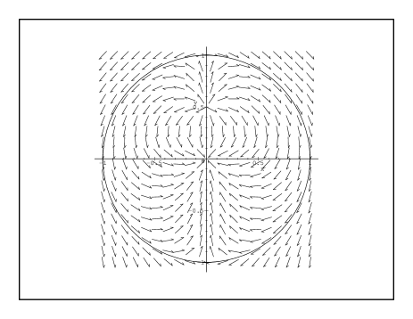
Figure 4: Directions of the field $D-E$ for $R=1$, $r_{0}=0.5$

Appendix B Renormalized energy for Neumann solutions

To compute integral (III.1):

$${\cal H}= m-\frac{1}{2}\int_{{\mathbb{R}^{3}}-V}D^{2}_{sing}dv+\frac{1}{2}\int_{V}D^{2}_{reg}dv+$$

$$+\int_{V}D_{sing}D_{reg}dv\ ,$$ (87)

observe that:

$$-\frac{1}{2}\int_{{\mathbb{R}^{3}}-V}D^{2}_{sing}dv=\frac{1}{2}\int_{{\partial\mathbb{R}^{3}}-\partial V}\phi_{sing}{D^{\bot}}_{sing}\,d\sigma\ ,$$ (88)

$$\frac{1}{2}\int_{V}D^{2}_{reg}dv=-\frac{1}{2}\int_{\partial V-{\partial\mathbb{R}^{3}}}\phi_{reg}{D^{\bot}}_{reg}\,d\sigma\ .$$ (89)

Integrals containing products of singular and regular fields are understood in the sense of distributions (cf. maurin , p. 748). Denoting $k_{\epsilon}:=K(\vec{r}_{0},\epsilon)$ we obtain:

$$\int_{V}D_{sing}D_{reg}dv=\lim_{\epsilon\rightarrow 0}\int_{V-k_{\epsilon}}D_{sing}D_{reg}dv=$$

$$=-\lim_{\epsilon\rightarrow 0}\frac{1}{2}\int_{V-k_{\epsilon}}\nabla\left(\phi_{sing}D_{reg}+\phi_{reg}D_{sing}\right)dv=$$

$$=-\lim_{\epsilon\rightarrow 0}\frac{1}{2}\int_{\partial V-\partial k_{\epsilon}}\left(\phi_{sing}{D^{\bot}}_{reg}+\phi_{reg}{D^{\bot}}_{sing}\right)\,d\sigma\ .$$ (90)

Hence, for $V=K_{R}:=K(0,R)$ we have:

$${\cal H}= m-\frac{1}{2}\int_{\partial K_{R}}\phi{D^{\bot}}\,d\sigma+$$

$$+\lim_{\epsilon\rightarrow 0}\frac{1}{2}\int_{\partial k_{\epsilon}}\left(\phi_{reg}D^{\bot}_{sing}+\phi_{sing}D^{\bot}_{reg}\right)\,d\sigma.$$ (91)

The formula is true for both the monopole and the dipole singularity of $D_{sing}$. Here, we consider the monopole (Coulomb) singularity. In this case the function $\phi_{sing}$ multiplied by $\epsilon^{2}$ (coming from the surface measure $d\sigma$) vanishes for $\epsilon\rightarrow 0$. Hence, we have:

$${\cal H}=m-\frac{1}{2}\int_{\partial K_{R}}\phi{D^{\bot}}\,d\sigma+\lim_{\epsilon\rightarrow 0}\frac{1}{2}\int_{\partial k_{\epsilon}}\phi_{reg}D^{\bot}_{sing}\,d\sigma\ .$$ (92)

To compute the integral over $\partial k_{\epsilon}$, we use spherical coordinates $(\epsilon,\beta,\varphi)$ centered at $\vec{r}_{0}$. Parameters $r$ and $\cos\theta$ present in $\phi_{reg}$ may be expressed as follows:

$$r^{2}=r_{0}^{2}+{\epsilon}^{2}-2{\epsilon}r_{0}\cos\beta,\qquad r\cos\theta=r_{0}-\epsilon\cos\beta\ ,$$ (93)

$$\lim_{\epsilon\rightarrow 0}r^{2}=r_{0}^{2},\qquad\lim_{\epsilon\rightarrow 0}r\cos\theta=r_{0}\ .$$ (94)

Then:

$$\lim_{\epsilon\rightarrow 0}\frac{1}{2}\int_{\partial k_{\epsilon}}\phi_{reg}D^{\bot}_{sing}\,d\sigma=$$

$$\lim_{\epsilon\rightarrow 0}\frac{e}{2}\frac{2\pi}{4\pi}\int_{0}^{\pi}\frac{1}{\epsilon^{2}}\phi_{reg}(r_{0},\epsilon,\beta)\sin\beta\epsilon^{2}\,d\beta=$$

$$=\frac{e}{4}\phi_{reg}(r_{0},r=r_{0},\theta=0)\int_{0}^{\pi}\sin\beta d\beta=\frac{1}{2}e\phi_{reg}{\big{|}}_{\vec{r}=\vec{r}_{0}}\ .$$ (95)

Consequently:

$${\cal H}=m-\frac{1}{2}\int_{\partial K_{R}}\phi{D^{\bot}}\,d\sigma+\frac{1}{2}e\phi_{reg}{\big{|}}_{\vec{r}=\vec{r}_{0}}.$$ (96)

Knowing $\phi$ we can compute ${\cal H}$:

$$D^{\bot}{|}_{r=R}=\frac{e}{4\pi}\frac{1}{R^{2}}+E\cos\theta,$$ (97)

$${\phi}{|}_{r=R}=-ER\cos\theta+$$

$$+\frac{e}{4\pi}\bigg{(}\frac{2}{\sqrt{R^{2}+{r_{0}}^{2}-2r_{0}R\cos\theta}}-\frac{1}{R}+\frac{1}{R}\ln(2R)+$$

$$-\frac{1}{R}\ln\left|R-r_{0}\cos\theta+\sqrt{R^{2}+{r_{0}}^{2}-2r_{0}R\cos\theta}\right|\bigg{)},$$ (98)

$$e\phi_{reg}{\big{|}}_{\vec{r}=\vec{r}_{0}}=$$

$$=-eEr_{0}+\frac{e^{2}}{4\pi}\left(\frac{R}{R^{2}-r_{0}^{2}}-\frac{1}{R}-\frac{1}{R}\ln\left|1-\frac{r_{0}^{2}}{R^{2}}\right|\right).$$ (99)

Note that:

$$\int_{K_{R}}\frac{1}{\sqrt{R^{2}+{r_{0}}^{2}-2r_{0}R\cos\theta}}d\sigma=4\pi R,$$ (100)

$$\int_{K_{R}}E\cos\theta d\sigma=0,$$ (101)

$$\int_{K_{R}}\ln\left|R-r_{0}\cos\theta+\sqrt{R^{2}+{r_{0}}^{2}-2r_{0}R\cos\theta}\right|d\sigma=$$

$$=4\pi R^{2}\ln 2R,$$

where we used two integrals $2.736$ from rizik . Then:

$$\frac{e}{4\pi R^{2}}\int_{K_{R}}\phi d\sigma =\frac{e^{2}}{4\pi R}.$$ (102)

Moreover:

$$E^{2}R\int_{K_{R}}\cos^{2}\theta d\sigma=\frac{4}{3}\pi R^{3}E^{2},$$ (103)

$$\int_{K_{R}}\frac{E\cos\theta}{\sqrt{R^{2}+{r_{0}}^{2}-2r_{0}R\cos\theta}}d\sigma=\frac{4}{3}\pi Er_{0},$$ (104)

$$\int_{K_{R}}\ln\left|R-r_{0}\cos\theta+\sqrt{R^{2}+{r_{0}}^{2}-2r_{0}R\cos\theta}\right|\times$$

$$\times E\cos\theta d\sigma=-\frac{4}{3}\pi r_{0}R,$$ (105)

where we used four integrals $2.736$ from rizik . Then:

$$E\int_{K_{R}} \phi\cos\theta d\sigma=-\frac{4}{3}\pi R^{3}E^{2}+\frac{eE}{4\pi}\left(\frac{8}{3}\pi r_{0}+\frac{4}{3}\pi r_{0}\right)=$$

$$=-\frac{4}{3}\pi R^{3}E^{2}+eEr_{0}.$$ (106)

The final result is the sum of (99), (102) and (B) with coefficient $\frac{1}{2}$:

$${\cal H}= m+\frac{1}{2}\left(\frac{e^{2}}{4\pi}\left(\frac{R}{R^{2}-r_{0}^{2}}-\frac{1}{R}\ln\left|1-\frac{r_{0}^{2}}{R^{2}}\right|-\frac{2}{R}\right)+\right.$$

$$+\left.\frac{4}{3}\pi R^{3}E^{2}-2eEr_{0}\right).$$ (107)

Appendix C Dirichlet solution and the corresponding energy

To find a solution of the Poisson equation $\Delta\phi=-e\delta(\vec{r}-\vec{r}_{0})$ with boundary conditions (22), where $\|\vec{r}_{0}\|<R$ and $\vec{r}_{0}\|\vec{E}$, we denote: $\phi=\phi_{sing}+\phi_{reg}^{0}-\vec{E}\vec{r}$, where $\phi_{sing}=\frac{1}{4\pi}\frac{e}{|\vec{r}-\vec{r}_{0}|}$, $\Delta\phi_{reg}^{0}=0$ and:

$$\phi_{reg}^{0}{\big{|}}_{r=R}=-\frac{1}{4\pi}\left(\frac{e}{|\vec{r}-\vec{r}_{0}|}\right){\bigg{|}}_{r=R}+\frac{e}{4\pi R}\ .$$ (108)

Again, we use Ansatz (78) as we did in Appendix A, page A, and expand also boundary conditions:

$$\phi_{reg}^{0}{\bigg{|}}_{r=R}=\frac{e}{4\pi}\left(\frac{1}{r}-\frac{1}{|\vec{r}-\vec{r}_{0}|}\right){\bigg{|}}_{r=R}\ ,$$ (109)

in series of Legendre polynomials. After substitution (77) and (78) to (109) we obtain:

$$\phi_{reg}^{0}=-\frac{eR}{4\pi}\sum_{n=1}^{\infty}\frac{{(rr_{0})}^{n}}{{(R^{2})}^{n+1}}P_{n}(\cos\theta).$$ (110)

After rescaling (77) we get:

$$\phi_{reg}^{0}=\frac{e}{4\pi}\left(\frac{1}{R}-\frac{R}{\sqrt{R^{4}+{r_{0}}^{2}r^{2}-2r_{0}rR^{2}\cos\theta}}\right).$$ (111)

Singular part of the electric field has the Coulomb singularity at $\vec{r}_{0}$. Hence, formula (96) is valid. However, we have:

$$D^{\bot}{|}_{r=R} =\frac{e}{4\pi R}\frac{R^{2}-r_{0}^{2}}{(R^{2}+{r_{0}}^{2}-2r_{0}R\cos\theta)^{\frac{3}{2}}}+E\cos\theta,$$ (112)

$${\phi}{|}_{r=R} =-ER\cos\theta+\frac{e}{4\pi}\frac{1}{R},$$ (113)

$$e\phi_{reg}{\big{|}}_{\vec{r}=\vec{r}_{0}} =-eEr_{0}+\frac{e^{2}}{4\pi}\left(\frac{1}{R}-\frac{R}{R^{2}-r_{0}^{2}}\right).$$ (114)

This implies:

$$2\pi R^{2} \int_{0}^{\pi}\frac{e^{2}}{(4\pi R)^{2}}\frac{(R^{2}-r_{0}^{2})\sin\theta\,d\theta}{(R^{2}+{r_{0}}^{2}-2r_{0}R\cos\theta)^{\frac{3}{2}}}=\frac{e^{2}}{4\pi R},$$ (115)

$$-2\pi R^{2} \int_{0}^{\pi}ER\cos\theta\,\frac{e}{4\pi R}\frac{(R^{2}-r_{0}^{2})\sin\theta\,d\theta}{(R^{2}+{r_{0}}^{2}-2r_{0}R\cos\theta)^{\frac{3}{2}}}=$$

$$=-eEr_{0},$$ (116)

$$-2\pi R^{2} \int_{0}^{\pi}E^{2}R\cos^{2}\theta\,\sin\theta\,d\theta=-\frac{4}{3}\pi R^{3}E^{2},$$ (117)

$$\int_{0}^{\pi}\cos\theta\,\sin\theta\,d\theta=0.$$ (118)

Consequently, we obtain:

$${\cal H}=m+\frac{1}{2}\left(\frac{4}{3}\pi R^{3}E^{2}-\frac{e^{2}}{4\pi}\frac{R}{R^{2}-r_{0}^{2}}\right)\ ,$$ (119)

or, in standardized variables (30),

$${\cal H_{D}^{\prime}}=\frac{1}{3}q^{2}-\frac{1}{1-x^{2}}.$$ (120)

Appendix D Dipole particle in a spherical box

We must solve equation $\Delta\phi^{dip}=\vec{p}\cdot\nabla\,(\delta(\vec{r}-\vec{r}_{0}))$ with boundary conditions $\vec{D}^{dip}\cdot\vec{n}{\big{|}}_{r=R}=0$. Denoting $\phi=\phi_{sing}^{dip}+\phi_{reg}^{dip}$, where

$$\phi_{sing}^{dip}=\frac{1}{4\pi}\frac{\vec{p}\cdot(\vec{r}-\vec{r}_{0})}{|\vec{r}-\vec{r}_{0}|^{3}}\ ,$$ (121)

we get Laplace equation $\Delta\phi_{reg}^{dip}=0$ with boundary condition:

$$\vec{D}_{reg}^{dip}\cdot\vec{n}{\big{|}}_{r=R}=\vec{n}\cdot\frac{1}{4\pi}\nabla\left(\frac{\vec{p}\cdot(\vec{r}-\vec{r}_{0})}{|\vec{r}-\vec{r}_{0}|^{3}}\right){\bigg{|}}_{r=R}\ .$$ (122)

For any pair of vectors $\vec{r}_{0}$ i $\vec{p}$ we choose coordinates in which $\vec{r}_{0}$ is parallel to the $z$-axis ${\bf e}_{z}$ and polarization vector assumes the form $\vec{p}=p{\boldsymbol{e}_{z}}+p_{x}{\boldsymbol{e}_{x}}$. The final solution will be the sum of two harmonic functions fulfilling boundary condition (122), calculated separately for $p{\boldsymbol{e}_{z}}$ and $p_{x}{\boldsymbol{e}_{x}}$.

Observe that, for $\phi^{mon}_{reg}(\vec{r}_{0},\vec{r})$ being a solution of Laplace equation, also the function $\frac{\vec{p}}{e}\cdot\nabla_{\vec{r}_{0}}\phi^{mon}_{reg}$ is harmonic. Moreover, if $\phi^{mon}_{reg}$ fulfills conditions ((79) condition from page 79):

$$\frac{\partial}{\partial r}\phi^{mon}_{reg}(\vec{r},\vec{r}_{0}){\bigg{|}}_{r=R}=\frac{e}{4\pi}\frac{\partial}{\partial r}\left(\frac{1}{r}-\frac{1}{|\vec{r}-\vec{r}_{0}|}\right){\bigg{|}}_{r=R}\ ,$$ (123)

then, after differentiation with respect to $\vec{r}_{0}$ we obtain:

$$-\frac{\partial}{\partial r} \left(\frac{\vec{p}}{e}\cdot\nabla_{\vec{r}_{0}}\phi^{mon}_{reg}\right){\bigg{|}}_{r=R}=$$

$$=\frac{1}{4\pi}\frac{\partial}{\partial r}\left(\vec{p}\cdot\nabla_{\vec{r}_{0}}\frac{1}{|\vec{r}-\vec{r}_{0}|}\right){\bigg{|}}_{r=R}\ .$$ (124)

Hence, the function $\frac{\vec{p}}{e}\cdot\nabla_{\vec{r}_{0}}\phi^{mon}_{reg}$ satisfies boundary conditions (122). We conclude that:

$$\phi_{reg}^{dip}=\frac{1}{4\pi e}\left(\vec{p}\cdot\nabla_{\vec{r}_{0}}\right)\phi_{reg}^{mon}\ ,$$ (125)

(cf. Panofsky , p.14). Applying (125) for $\vec{p}=p{\boldsymbol{e}_{z}}+p_{x}{\boldsymbol{e}_{x}}$ allows us to solve the problem separately for $p$ parallel and orthogonal to $\vec{r}_{0}$.

D.1 Solution for $\vec{p}\parallel\vec{r}_{0}$

To obtain the parallel part we differentiate monopole solution ((A), Appendix A) along the ${\bf e}_{z}$-axis:

$$\phi_{reg}^{dip}=\frac{p}{e}\,\frac{\partial}{\partial r_{0}}\phi^{mon}_{reg}=$$

$$\frac{p}{4\pi}\frac{\partial}{\partial r_{0}}\bigg{(}\frac{R}{\sqrt{R^{4}+{r_{0}}^{2}r^{2}-2r_{0}rR^{2}\cos\theta}}-\frac{1}{R}+\frac{1}{R}\ln(2R^{2})$$

$$-\frac{1}{R}\ln\left|R^{2}-r_{0}r\cos\theta+\sqrt{R^{4}+{r_{0}}^{2}r^{2}-2r_{0}rR^{2}\cos\theta}\right|\bigg{)}$$

$$=\frac{p}{4\pi}\bigg{(}-\frac{R(r_{0}r^{2}-rR^{2}\cos\theta)}{(R^{4}+{r_{0}}^{2}r^{2}-2r_{0}rR^{2}\cos\theta)^{\frac{3}{2}}}+$$

$$-\frac{1}{R\sqrt{R^{4}+{r_{0}}^{2}r^{2}-2r_{0}rR^{2}\cos\theta}}\times$$

$$\frac{-r\cos\theta\left(\sqrt{R^{4}+{r_{0}}^{2}r^{2}-2r_{0}rR^{2}\cos\theta}+R^{2}\right)+r^{2}r_{0}}{R^{2}-rr_{0}\cos\theta+\sqrt{R^{4}+{r_{0}}^{2}r^{2}-2r_{0}rR^{2}\cos\theta}}\bigg{)}.$$ (126)

But:

$$\left(R^{2}-rr_{0}\cos\theta+\sqrt{R^{4}+{r_{0}}^{2}r^{2}-2r_{0}rR^{2}\cos\theta}\right)\times$$ (127)

$$\times\left(R^{2}-rr_{0}\cos\theta-\sqrt{R^{4}+{r_{0}}^{2}r^{2}-2r_{0}rR^{2}\cos\theta}\right)=$$

$$=-(r_{0}r)^{2}\sin^{2}\theta,$$ (128)

$$\left(-r\cos\theta\left(\sqrt{R^{4}+{r_{0}}^{2}r^{2}-2r_{0}rR^{2}\cos\theta}+R^{2}\right)+r^{2}r_{0}\right)$$

$$\times\left(R^{2}-rr_{0}\cos\theta-\sqrt{R^{4}+{r_{0}}^{2}r^{2}-2r_{0}rR^{2}\cos\theta}\right)=$$

$$=-r_{0}r^{2}\sin^{2}\theta\sqrt{R^{4}+{r_{0}}^{2}r^{2}-2r_{0}rR^{2}\cos\theta}+$$

$$r\cos\theta(-r_{0}rR^{2}\cos\theta)+R^{2}r^{2}r_{0}=$$

$$=r^{2}r_{0}\sin^{2}\theta\left(R^{2}-\sqrt{R^{4}+{r_{0}}^{2}r^{2}-2r_{0}rR^{2}\cos\theta}\right).$$ (129)

So:

$$\phi_{reg}^{dip}=\frac{p}{4\pi}\bigg{(}-\frac{R(r_{0}r^{2}-rR^{2}\cos\theta)}{(R^{4}+{r_{0}}^{2}r^{2}-2r_{0}rR^{2}\cos\theta)^{\frac{3}{2}}}+$$

$$+\frac{r^{2}r_{0}\sin^{2}\theta\,(R^{2}-\sqrt{R^{4}+{r_{0}}^{2}r^{2}-2r_{0}rR^{2}\cos\theta})}{R(rr_{0})^{2}\sin^{2}\theta\,\sqrt{R^{4}+{r_{0}}^{2}r^{2}-2r_{0}rR^{2}\cos\theta}}\bigg{)}=$$

$$=\frac{1}{4\pi}\left(\frac{p\,R^{3}\left(R^{2}-rr_{0}\cos\theta\right)}{r_{0}\left(R^{4}+(r_{0}r)^{2}-2rr_{0}R^{2}\cos\theta\right)^{\frac{3}{2}}}-\frac{p}{r_{0}R}\right).$$ (130)

Figure 5 shows the directions of the field $D^{dip}$. Observe that the field is tangent to the boundary of $K(0,R)$.

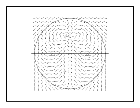
Figure 5: Directions of the field $D_{sing}^{dip}+D_{reg}^{dip}$, $R=1$, $r_{0}=0.5$, $p=1$

D.2 Solutions for $\vec{p}\bot\vec{r_{0}}$

For $\vec{p}=p_{x}{\boldsymbol{e}_{x}}$ we get:

$$\phi_{reg}^{dip}=p_{x}\frac{{\boldsymbol{e}_{x}}}{e}\cdot\nabla_{\vec{r}_{0}}\phi_{reg}^{mon}=\frac{p_{x}}{e}\frac{\partial}{\partial x_{0}}\phi_{reg}^{mon}.$$ (131)

The easiest way to calculate this derivative is to use spherical coordinates $\vec{r}_{0}=(r_{0},\theta_{0},\varphi_{0})$. Then:

$$x_{0} =r_{0}\sin\theta_{0}\sin\varphi_{0}\&,\quad y_{0}=r_{0}\sin\theta_{0}\cos\varphi_{0}\ ,$$

$$z_{0} =r_{0}\cos\theta_{0}\ ,$$ (132)

and:

$$\frac{\partial}{\partial x_{0}} =\sin\theta_{0}\cos\varphi_{0}\frac{\partial}{\partial r_{0}}+\cos\theta_{0}\cos\varphi_{0}\frac{1}{r_{0}}\frac{\partial}{\partial\theta_{0}}+$$

$$-\frac{\sin\varphi_{0}}{r_{0}\sin\theta_{0}}\frac{\partial}{\partial\varphi_{0}}\ .$$ (133)

But for $\vec{r}_{0}\|{\bf e}_{z}$ this procedure is singular because $\sin\theta_{0}=0$. To overcome this difficulty we first calculate the result for $\vec{r}_{0}\nparallel{\bf e}_{z}$ and then pass to the limit $\theta_{0}\rightarrow 0$ and $\varphi_{0}\rightarrow 0$. For this purpose we must be able to differentiate the function $\cos\gamma$, where $\gamma$ is the angle between $\vec{r}$ and $\vec{r}_{0}$, i.e.:

$$\vec{r}\cdot\vec{r}_{0}=rr_{0}\cos\gamma\ ,$$ (134)

or, equivalently:

$$\cos\gamma=\cos\theta\cos\theta_{0}+\sin\theta\sin\theta_{0}\cos(\varphi-\varphi_{0})\ .$$ (135)

Hence, (133) gives us:

$$\frac{\partial}{\partial x_{0}}\cos\gamma=$$

$$\bigg{(}\frac{1}{r_{0}}\cos\theta\cos\varphi_{0}\left(-\cos\theta\sin\theta_{0}+\sin\theta\cos\theta_{0}\cos(\varphi-\varphi_{0})\right)$$

$$-\frac{1}{r_{0}}\sin\varphi_{0}\sin\theta\sin(\varphi-\varphi_{0})\bigg{)}\overset{\theta_{0}\rightarrow 0}{\underset{\varphi_{0}\rightarrow 0}{\longrightarrow}}\frac{1}{r_{0}}\sin\theta\cos\varphi.$$ (136)

This method allows us to calculate effectively the derivative of the monopole field from Appendix A (p. A) along $x_{0}$. The final result reads:

$$\phi_{reg}^{dip}=\frac{p_{x}}{4\pi}\Bigg{(}\frac{rR^{3}\sin\theta\cos\varphi}{(R^{4}+{r_{0}}^{2}r^{2}-2r_{0}rR^{2}\cos\theta)^{\frac{3}{2}}}+$$

$$-\frac{\cos\varphi(R^{2}\cos\theta-r_{0}r)}{Rr_{0}\sin\theta\sqrt{R^{4}+{r_{0}}^{2}r^{2}-2r_{0}rR^{2}\cos\theta}}+\frac{\cos\theta\cos\varphi}{Rr_{0}\sin\theta}\Bigg{)}.$$ (137)

We stress that the above function is regular at $\theta=0$ due to cancellations between the second and the third term.

Appendix E Renormalized energy of a dipole particle

To calculate ${\cal H}^{dip}$ we use results of Appendix B. It turns out that in formula (B), only the following non-vanishing terms were not taken into account in ${\cal H}^{mon}$:

$${\cal H}^{dip}=-\frac{1}{2}\int_{\partial K_{R}}\phi^{dip}{D^{\bot}}\,d\sigma+$$

$$+\lim_{\epsilon\rightarrow 0}\frac{1}{2}\int_{\partial k_{\epsilon}}\left(\phi^{dip}_{reg}D^{\bot\,mon}_{sing}+\phi^{dip}_{sing}D^{\bot}_{reg}\right)\,d\sigma\ ,$$ (138)

where:

$$\phi^{dip}_{reg}=\frac{1}{4\pi}\left(\frac{p\,R^{3}\left(R^{2}-rr_{0}\cos\theta\right)}{r_{0}\left(R^{4}+(r_{0}r)^{2}-2rr_{0}R^{2}\cos\theta\right)^{\frac{3}{2}}}-\frac{p}{r_{0}R}\right),$$ (139)

$$\phi^{dip}_{sing}=\frac{1}{4\pi}\frac{p(r\cos\theta-r_{0})}{(r^{2}+r_{0}^{2}-2rr_{0}\cos\theta)^{\frac{3}{2}}},$$ (140)

$$\phi^{mon}_{reg}=\frac{e}{4\pi}\bigg{(}\frac{R}{\sqrt{R^{4}+{r_{0}}^{2}r^{2}-2r_{0}rR^{2}\cos\theta}}-\frac{1}{R}+$$

$$-\frac{1}{R}\ln\left|R^{2}-r_{0}r\cos\theta+\sqrt{R^{4}+{r_{0}}^{2}r^{2}-2r_{0}rR^{2}\cos\theta}\right|\bigg{)}$$

$$-Er\cos\theta+\frac{1}{R}\ln(2R^{2}),$$ (141)

$$\phi^{dip}=\phi^{dip}_{reg}+\phi^{dip}_{sing}\ .$$ (142)

Moreover, we have:

$$D^{\bot}{\big{|}}_{\partial K_{R}} = \frac{1}{4\pi}\frac{e}{R^{2}}+E\cos\theta\ ,$$ (143)

$$D^{\bot}_{reg}{\big{|}}_{\partial k_{\epsilon}} = -\frac{\partial}{\partial\epsilon}\left(\phi^{mon}_{reg}+\phi^{dip}_{reg}\right)\ .$$ (144)

To compute the integral over $\partial K_{R}$ we note that:

$$\phi^{dip}{\bigg{|}}_{r=R}=$$

$$\phi^{dip}_{reg}+\phi^{dip}_{sing}=\frac{p}{4\pi r_{0}}\left(\frac{R^{2}-r_{0}^{2}}{(R^{2}+r_{0}^{2}-2Rr_{0}\cos\theta)^{\frac{3}{2}}}-\frac{1}{R}\right),$$ (145)

whereas $D^{\bot}$ is expressed by (143). Moreover:

$$\frac{1}{4\pi}\frac{e}{R^{2}}2\pi\int_{0}^{\pi}\phi^{dip}\sin\theta\,d\theta=0.$$ (146)

So:

$$-\frac{1}{2}2\pi\,E\int_{0}^{\pi}\phi^{dip}\cos\theta\sin\theta\,d\theta=-\frac{1}{2}p\,E.$$

To find the limit:

$$\lim_{\epsilon\rightarrow 0}\frac{1}{2}\int_{\partial k_{\epsilon}}\left(\phi^{dip}_{sing}D^{\bot}_{reg}+D^{mon}_{sing}\phi^{dip}_{reg}\right)\,d\sigma,$$ (147)

we analyze behaviour of fields (139) - (144) for $\epsilon\rightarrow 0$. All these terms have at most the $\epsilon^{-2}$-singularity. Therefore, they are continuous and bounded when multiplied by $\epsilon^{2}$. Thus, we can interchange the limit and the integration operations.

We follow our procedure described in Appendix B, page B. Using (93) and (94) we obtain in terms of the standardized variable $x=\frac{r_{0}}{R}$:

$$\lim_{\epsilon\rightarrow 0}\left(\epsilon^{2}\,\phi^{dip}_{sing}\right)=-\frac{p}{4\pi}\cos\beta,$$ (148)

$$\lim_{\epsilon\rightarrow 0}\left(-\frac{\partial}{\partial\epsilon}\phi^{mon}_{reg}\right)=$$

$$\frac{e}{4\pi}\left(\frac{r_{0}R}{(R^{2}-r_{0}^{2})^{2}}+\frac{r_{0}}{(R^{2}-r_{0}^{2})^{2}R}\right)\cos\beta-E\cos\beta=$$

$$\left(\frac{e}{4\pi}\frac{1}{R^{2}}\frac{x(2-x^{2})}{(1-x^{2})^{2}}-E\right)\cos\beta=-\cos\beta\,D^{mon}_{reg}{\bigg{|}}_{\vec{r}=\vec{r_{0}}},$$ (149)

$$\lim_{\epsilon\rightarrow 0}\left(-\frac{\partial}{\partial\epsilon}\phi^{dip}_{reg}\right)=\frac{1}{4\pi}\frac{2pR^{3}}{(R^{2}-r_{0}^{2})^{3}}\cos\beta=$$

$$=\frac{1}{4\pi}\frac{2p}{R^{3}(1-x^{2})^{3}}\cos\beta=-\cos\beta\,D^{dip}_{reg}{\bigg{|}}_{\vec{r}=\vec{r_{0}}},$$ (150)

$$\lim_{\epsilon\rightarrow 0}\left(\epsilon^{2}\,D^{mon}_{sing}\right)=\frac{e}{4\pi},$$ (151)

$$\lim_{\epsilon\rightarrow 0}\left(\phi^{dip}_{reg}\right)=\frac{1}{4\pi}\frac{pr_{0}(2R^{2}-r_{0}^{2})}{R(R^{2}-r_{0}^{2})^{2}}=$$

$$\frac{p}{4\pi}\frac{x(2-x^{2})}{R^{2}(1-x^{2})^{2}}=-\frac{p}{e}D^{mon}_{reg}{\bigg{|}}_{\vec{r}=\vec{r_{0}}},$$ (152)

$$\int_{0}^{\pi}\cos^{2}\beta\sin\beta\,d\beta=\frac{2}{3}.$$ (153)

Then:

$$\frac{1}{2}\int_{\partial k_{\epsilon}}\left(\phi^{dip}_{sing}D^{\bot}_{reg}+D^{mon}_{sing}\phi^{dip}_{reg}\right)\,d\sigma=$$

$$=\frac{1}{2}\left(\frac{4\pi}{3}\frac{p}{4\pi}\left(D^{mon}_{reg}{\bigg{|}}_{\vec{r}=\vec{r_{0}}}+D^{dip}_{reg}{\bigg{|}}_{\vec{r}=\vec{r_{0}}}\right)\right.+$$

$$\left.-\frac{e}{4\pi}4\pi\frac{p}{e}D^{mon}_{reg}{\bigg{|}}_{\vec{r}=\vec{r_{0}}}\right)=$$

$$=\frac{1}{2}\left(\frac{pe}{4\pi}\frac{1}{R^{2}}\frac{2}{3}\frac{x(2-x^{2})}{(1-x^{2})^{2}}-\frac{1}{4\pi}\frac{1}{3}\frac{2p^{2}}{R^{3}(1-x^{2})^{3}}+\frac{1}{3}p\,E\right).$$ (154)

Using $q=\frac{4\pi R^{2}}{e}E$ and (31) we obtain:

$${\cal H}^{\prime\ dip}:=\frac{8\pi R}{e^{2}}{\cal H}^{dip}=\frac{2}{3}\left(\frac{p}{eR}\frac{x(2-x^{2})}{(1-x^{2})^{2}}-\frac{p^{2}}{e^{2}R^{2}}\frac{1}{(1-x^{2})^{3}}-\frac{p}{eR}\,q\right).$$ (155)

References

- (1) P. A. M. Dirac, Classical theory of radiating electrons, (Proc. Roy. Soc. A 167 (1938), 148–169).
- (2) H. P. Gittel, J. Kijowski, E. Zeidler, The relativistic dynamics of the combined particle-field system in renormalized classical electrodynamics, (Commun. Math. Phys. 198 (1998), 711–736).
- (3) R. Haag, Die Selbstwechselwirkung des Elektrons, (Naturforsch. 10 a (1955), 752–761).
- (4) J. Kijowski, Electrodynamics of moving particles, (Gen. Rel. Grav. 26 (1994), 167–201. See also On electrodynamical self–interaction, Acta Phys. Pol. A 85 (1994), 771–787).
- (5) J. Kijowski, M. Kościelecki, Asymptotic expansion of the Maxwell field in a neighbourhood of a multipole particle, (Acta. Phys. Polon. B 31 (2000), 1691 – 1707).
- (6) J. Kijowski, M. Kościelecki, Algebraic description of the Maxwell field singularity in a neighbourhood of a multipole particle, (Rep. Math. Phys. 47 (2001), 301–311).
- (7) M. Kościelecki, Master’s Thesis, (Warsaw University (1995)).
- (8) M. Kościelecki, Ph. D. Thesis, (Warsaw University (2001)).
- (9) J. Kijowski, P. Podleś, Born renormalization in classical Maxwell electrodynamics, (Journal Geom. Phys, in print).
- (10) F. Rohrlich, Classical Charged Particles. Foundations of Their Theory, (Addison–Wesley, Reading 1965).
- (11) W. K. H. Panofsky, Classical electricity and magnetism, (Addison – Wesley, Inc. 1962).
- (12) I. S. Gradsztejn, I. M. Ryzhik, Tablicy integralow, summ …, (Nauka, Moskwa 1971).
- (13) K. Maurin, Analysis, part II, (PWN, Warszawa (1980)).