Streamer Branching rationalized by Conformal Mapping Techniques

Abstract

Spontaneous branching of discharge channels is frequently observed, but not well understood. We recently proposed a new branching mechanism based on simulations of a simple continuous discharge model in high fields. We here present analytical results for such streamers in the Lozansky-Firsov limit where they can be modelled as moving equipotential ionization fronts. This model can be analyzed by conformal mapping techniques which allow the reduction of the dynamical problem to finite sets of nonlinear ordinary differential equations. Our solutions illustrate that branching is generic for the intricate head dynamics of streamers in the Lozansky-Firsov-limit.

When non-ionized matter is suddenly exposed to strong fields, ionized regions can grow in the form of streamers. These are ionized and electrically screened channels with rapidly propagating tips. The tip region is a very active impact ionization region due to the self-generated local field enhancement. Streamers appear in early stages of atmospheric discharges like sparks or sprite discharges [1, 2], they also play a prominent role in numerous technical processes. It is commonly observed that streamers branch spontaneously [3, 4]. But how this branching is precisely determined by the underlying discharge physics, is essentially not known. In recent work [5, 6], we have suggested a branching mechanism from first principles. This work drew some attention [7, 8], since the proposed mechanism yields quantitative predictions for specific parameters, and since it is qualitatively different from the older branching concept of the “dielectric breakdown model” [9, 10, 11]. This older concept actually can be traced back to concepts of rare long-ranged (and hence stochastic) photo-ionization events probably first suggested in 1939 by Raether [12]. Therefore, it came as a surprise that we predicted streamer branching in a fully deterministic model. Since our evidence for the phenomenon was mainly from numerical solutions together with a physical interpretation, the accuracy of our numerical scheme was challenged [13, 14]. Furthermore, some authors have argued previously [15, 16] that in a deterministic discharge model like ours, an initially convex streamer head never could become locally concave, and that hence the consecutive branching of the discharge channel would be unphysical.

Therefore in the present paper, we investigate the issue by analytical means. We show that the convex-to-concave evolution of the streamer head with successive branching is generic for streamers in the Lozansky-Firsov limit [5, 6, 17]. We define the Lozansky-Firsov-limit as the stage of evolution where the streamer head is almost equipotential and surrounded by a thin electrostatic screening layer. While in the original article [17], only simple steady state solutions with parabolic head shape are discussed, we will show here that a streamer in the Lozansky-Firsov limit actually can exhibit a very rich head dynamics that includes spontaneous branching. Furthermore, our analytical solutions disprove the reasoning of [15] by explicit counterexamples. Our analytical methods are adapted from two fluid flow in Hele-Shaw cells [18, 19, 20, 21, 22]. But our explicit and exact solutions that amount to the evolution of “bubbles” in a dipole field [23], have not been reported in the hydrodynamics literature either.

The relation between our previous numerical investigations [5, 6] and our present analytical model is laid in two steps. First, numerical solutions show essentially the same evolution in the purely two-dimensional case as in the three-dimensional case with assumed cylinder geometry [5, 6]. Because there is an elegant analytical approach, we focus on the two-dimensional case. This has the additional advantage that such two-dimensional solutions rather directly apply to, e.g., discharges in Corbino discs [24]. Second, we use the following simplifying approximations for a Lozansky-Firsov streamer: $(1)$ the interior of the streamer is electrically completely screened; hence the electric potential $\varphi$ is constant; hence the ionization front coincides with an equipotential line, $(2)$ the width of the screening layer around the ionized body is much smaller than all other relevant length scales and in the present study it is actually neglected, $(3)$ the velocity of the ionization front v is determined by the local electric field; in the simplest case to be investigated here, it is simply taken to be proportional to the field at the boundary ${\bf v}=c\;\nabla\varphi$ with some constant $c$ (for the validity of the approximation, cf. [25, 26]). Together with $\nabla^{2}\varphi=0$ in the non-ionized outer region and with fixed limiting values of the potential $\varphi$ far from the streamer, this defines a moving boundary problem for the interface between ionized and non-ionized region. We assume the field far from the streamer to be constant as in our simulations [6]. Such a constant far field can be mimicked by placing the streamer between the two poles of an electric dipole where the distance between the poles is much larger than the size of the streamer.

When the electric field points into the $x$ direction and $y$ parametrizes the transversal direction, our two-dimensional Lozansky-Firsov streamer in free flight in a homogeneous electric field is approximated by:

$$\nabla^{2}\varphi(x,y)=0, \mbox{outside the streamer},$$ (1)

$$-\nabla\varphi(x,y)\rightarrow E_{0}\hat{x}, \mbox{far outside the streamer},$$ (2)

$$\varphi(x,y)=0, \mbox{inside the streamer},$$ (3)

$${\bf v}_{\rm bound.}=c\;\nabla\varphi\big{|}_{\rm bound.}, \mbox{velocity of the boundary},$$ (4)

where $\hat{x}$ is the unit vector in the $x$ direction, and we have chosen the gauge such that the potential inside the streamer vanishes. The asymptote (2) implies that the total charge on the streamer vanishes; otherwise a contribution $\propto 1/\sqrt{x^{2}+y^{2}}$ has to be added on the r.h.s. of Eq. (2).

Similar moving boundary problems arise in Hele-Shaw flow of two fluids with a large viscosity contrast [18, 19]: Lozansky-Firsov streamers and viscous fingers on the present level of description can be identified immediately by equating the electric potential $\varphi$ with the fluid pressure $p$ [25, 26]. To such problems, powerful conformal mapping methods [20, 21, 22] can be applied. Most work with this method is concerned with viscous fingers in a channel geometry, i.e., with boundary conditions on a lateral external boundary that cannot be realized in an electric system. A few authors also study air bubbles within a viscous fluid, or viscous droplets in air, mostly under the action of flow fields generated by one source or one sink of pressure, i.e., by monopoles. On the other hand, the approximation (1)-(4) describes streamers in free space between two electrodes as in [6]. With the asymptote (2), this is mathematically equivalent to air bubbles in a dipole field. This case has not been studied in detail. It is known that any ellipse with the main axes oriented parallel and perpendicular to the direction of the dipole is a uniformly translating solution of this problem [27]. The time dependent solutions of [28] do not apply to streamers since the boundary condition on the moving interface is different. Refs. [23] and [29] study how and when cusps in the interfaces of droplets and bubbles emerge when these are driven by multipole fields. But for bubbles in a dipole field, again only the steady state ellipse solutions are given [23].

In the present paper, we therefore apply conformal mapping methods to the evolution of “bubbles” in a dipole field in a Hele-Shaw experiment and proceed beyond the steady state ellipse solutions. We identify the general structure of time dependent solutions of (1)-(4). The analytically derived exact solutions show how a streamer head can become flatter, concave and branch as observed numerically [5, 6]. Rather than a pole decomposition [20], we derive a decomposition into Fourier modes of the circle and calculate an equation for the non-linear dynamical coupling of their amplitudes.

In detail, this is done in the following steps:
$(i)$ The spatial coordinates are expressed by the complex coordinate $z=x+iy$. According to standard complex analysis, finding a real harmonic function $\varphi(x,y)$ solving the Laplace equation (1) in a given region is equivalent to finding a complex function $\Phi(z)$ that is analytical in the same region and has real part ${\rm Re}\;\Phi(z)=\varphi(x,y)$.
$(ii)$ A conformal map from the interior of the unit circle to the exterior of the streamer or “bubble” is constructed. Including the point at infinity, the region outside the streamer is simply connected and Riemann’s mapping theorem applies; therefore the mapping exists. Since the boundary moves, the mapping is time dependent; we denote it with $z=f_{t}(\omega)$ where $\omega$ parametrizes the interior of the unit circle $|\omega|<1$. The complete map can be composed from a conformal map $\zeta=h_{t}(\omega)$ that deforms the unit disc continuously, followed by the inversion $z=1/\zeta$. Since $h_{t}(\omega)$ is conformal on the unit disc, it is analytical and has a single zero which we choose to be at $\omega=0$. Therefore $f_{t}(\omega)=1/h_{t}(\omega)$ has a single pole $\propto\omega^{-1}$ and is otherwise analytical. Rather than a pole decomposition [20], we choose a Laurent expansion for $f_{t}(\omega)$

$$x+iy=z=f_{t}(\omega)=\sum_{k=-1}^{\infty}a_{k}(t)\;\omega^{k}.$$ (5)

This expansion allows us to identify the exact dynamical solutions (12) below. Taking $a_{-1}(t)$ as a real positive number makes the mapping unique, again according to Riemann’s mapping theorem.
$(iii)$ Now the potential $\hat{\Phi}(\omega)$ on the unit disc can be calculated explicitly. Since $f_{t}(\omega)$ is a conformal mapping, the function $\Phi(z)$ is analytical if and only if the function $\hat{\Phi}(\omega)=\Phi(f_{t}(\omega))$ is analytical. The asymptote of $\hat{\Phi}(\omega)$ for $\omega\to 0$ is determined by (2) and (5): for $|x|,|z|\to\infty$, we have $\varphi(x,y)\to-E_{0}x$, hence $\Phi(z)\to-E_{0}z$, and therefore with (5): $\hat{\Phi}(\omega)\to-E_{0}a_{-1}(t)/\omega$ for $\omega\to 0$. This means that the pole of $\hat{\Phi}(\omega)$ at the origin of the unit disc $\omega=0$ corresponds to the dipole of $\Phi(z)$ at $z\to\pm\infty$. This dipole generates the field and the interfacial motion. In the remainder of the unit disc, there are no sources or sinks of potential, hence $\hat{\Phi}$ is analytical there. Furthermore, at the boundary of the streamer, we have $\varphi=0$ from (3) or ${\rm Re}\;\Phi=0$, resp. The boundary of the streamer maps onto the unit circle, so ${\rm Re}\;\hat{\Phi}(\omega)=0$ for $|\omega|=1$. Using the asymptotics at $\omega\to 0$ and analyticity in the remaining region, the unique and exact solution for the potential is

$$\hat{\Phi}(\omega)=E_{0}a_{-1}(t)\left(\omega-\frac{1}{\omega}\right).$$ (6)

$(iv)$ The velocity ${\bf v}_{\rm bound.}=c\nabla\phi$ (4) determines the motion of the interface. This interface is the time dependent map $f_{t}(\omega)$ of the unit circle $\omega=e^{i\alpha}$ parametrized by the angle $\alpha\in[0,2\pi)$. Therefore Eq. (4) determines the dynamics of $f_{t}\left(e^{i\alpha}\right)$. According to [18, 20], it is

$${\rm Re}\;\Big{[}\!-i\partial_{\alpha}f_{t}^{*}\big{(}e^{i\alpha}\big{)}\;\partial_{t}f_{t}\big{(}e^{i\alpha}\big{)}\Big{]}=c\;{\rm Re}\;\Big{[}i\partial_{\alpha}\hat{\Phi}\big{(}e^{i\alpha}\big{)}\Big{]}.$$ (7)

The problem (1)-(4) is symmetric under reflection on the $x$-axis. We assume the solutions to have the same symmetry. Therefore all $a_{k}(t)$ have to be real. The position $(x,y)(\alpha,t)$ of the point of the interface labelled by the angle $\alpha$ at time $t$ can be read directly from the Laurent expansion (5) by inserting $\omega=e^{i\alpha}$; it has essentially the form of a Fourier expansion of the unit circle where the circle and its position are created by the modes $k=-1$ and 0:

$$x(\alpha,t)=\!\sum_{k=-1}^{\infty}\!a_{k}(t)\;\cos k\alpha~{}~{},~{}~{}y(\alpha,t)=\!\sum_{k=-1}^{\infty}\!a_{k}(t)\;\sin k\alpha,$$ (8)

$$~{}~{}~{}a_{k}(t)~{}\mbox{real}~{}~{},~{}~{}a_{-1}(t)>0~{}~{}~{},~{}~{}~{}0\leq\alpha<2\pi~{}.$$ (9)

Substituting the mapping function (5) and the potential (6) into the equation of motion for the mapping (7), and assuming the $a_{k}(t)$ to be real, we obtain for the evolution of the amplitudes $a_{k}(t)$:

$$\sum_{k,k^{\prime}=-1}^{\infty}k^{\prime}a_{k^{\prime}}(t)\;\partial_{t}a_{k}(t)\;\cos\big{(}(k-k^{\prime})\alpha\big{)}$$ (10)

$$\qquad\qquad=2E_{0}c\;a_{-1}(t)\;\cos\alpha.$$ (11)

A closer investigation shows that this equation has an important property: suppose that the streamer boundary can be written initially as a finite series $\sum_{k=-1}^{N}a_{k}(0)\;e^{ik\alpha}$, $a_{N}(0)\neq 0$. Then at all times $t$, the interface is described by the same finite number of modes

$$z(\alpha,t)=\sum_{k=-1}^{N}a_{k}(t)\;e^{ik\alpha},$$ (12)

i.e., the $a_{k}(t)$ with $k>N$ stay identical to zero at all times $t>0$. Sorting the terms in (10) by coefficients of $\cos k\alpha$, the equation can be recast into $N+2$ ordinary differential equations for the $N+2$ functions $a_{k}(t)$

$$\sum_{k=-1}^{N-m}\Big{[}(k+m)\;a_{k+m}\;\partial_{t}a_{k}+k\;a_{k}\;\partial_{t}a_{k+m}\Big{]}$$ (14)

$$~{}~{}=2E_{0}c\;a_{-1}\;\delta_{m,1}~{}~{}~{}~{}\mbox{ for }m=0,\ldots,N+1,$$

where $\delta_{m,1}$ is the Kronecker symbol. Eq. (14) is equivalent to a matrix equation of the form ${\bf A}(\{a_{k}(t)\})\cdot\partial_{t}\Big{(}a_{-1}(t),\ldots,a_{N}(t)\Big{)}=\Big{(}0,2E_{0}ca_{-1}(t),0,\ldots,0\Big{)}$, where the matrix ${\bf A}$ depends linearly on the $\{a_{k}(t)\}$.

Eqs. (12) and (14) identify large classes of analytical solutions with arbitrary fixed $N$. These solutions reduce the dynamical moving boundary problem in two spatial dimensions of Eqs. (1)–(4) exactly to a finite set of ordinary differential equations for the nonlinear coupling of the amplitudes $a_{k}(t)$ of modes $e^{ik\alpha}$, $0\leq\alpha<2\pi$. These equations are easy to integrate numerically or for small $N$ even analytically. We will use this form to discuss now generic solutions of Eqs. (1)–(4) as the simplest approximation of a streamer in the Lozansky-Firsov limit.

First, it is now easy to reproduce the uniformly propagating ellipse solutions of [23, 27] as the solutions with $N=1$: for $|a_{1}|\neq|a_{-1}|$, the equations reduce to $\partial_{t}a_{-1}=0=\partial_{t}a_{1}$ and $\partial_{t}a_{0}=2E_{0}c\;a_{-1}/(a_{1}-a_{-1})$. These solutions correspond to ellipses whose principal radii are oriented along the axes. These radii maintain their values $r_{x,y}=a_{-1}\pm a_{1}$ (assuming $a_{-1}>a_{1}>0$) and move with constant velocity $v_{\rm ellipse}=-E_{0}c\;(r_{x}+r_{y})/r_{y}$. The Lozansky-Firsov-parabola can be understood as limit cases of such uniformly propagating ellipses.

In contrast to $N\leq 1$, all solutions with $N\geq 2$ have nontrivial dynamics. It can be tracked by integrating the $N+2$ ordinary differential equations (14) numerically and then plotting the boundaries (12) at consecutive times. Examples of such dynamics are shown in the figures.

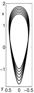
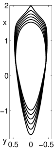
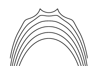
FIG. 1.: Upper panel: evolution of the interface in equal time steps up to time $t=0.1/(E_{0}c)$ with initial condition
a) $z_{0}(\alpha,0)=e^{-i\alpha}+0.6\cdot e^{i\alpha}-0.08\cdot e^{2i\alpha}$,
b) $z(\alpha,0)=z_{0}(\alpha,0)-5\cdot 10^{-3}\cdot e^{8i\alpha}$
c) $z(\alpha,0)=z_{0}(\alpha,0)+3\cdot 10^{-3}\cdot e^{8i\alpha}$
d) $z(\alpha,0)=z_{0}(\alpha,0)-4.5\cdot 10^{-7}\cdot e^{30i\alpha}$,
and lower panel: zoom into the unstable head of Fig. d.

Fig. 1 shows four cases of the upward motion of a conically shaped streamer in equal time steps. The initial conditions are almost identical. On the leftmost figure, an ellipse is corrected only by a mode $e^{2i\alpha}$ to create the conical shape. This shape with $N=2$ eventually develops a concave tip, but only after much longer times than shown in the figure. In the other figures this conical shape is perturbed initially by a minor perturbation with wavenumber 8 or 30, corresponding to $N=8$ and 30 in (12) and (14). The amplitude of the perturbation is chosen such that a cusp develops at time $0.1/(E_{0}c)$. Depending on the sign of the amplitude, the cusp develops on or off axis — where we stress that we are not interested in the cusp itself, but in the earlier stages of evolution. Note that our reduction of the moving boundary problem to the set of ordinary differential equations (14) assures that the evolving shape is a true solution of the problem (1)–(4). Figs. $1b$ and $1d$ demonstrate that spontaneous branching is a possible solution.

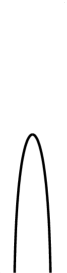
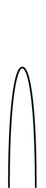
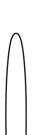
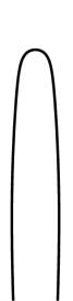
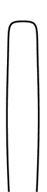
FIG. 2.: Evolution of the tip of an elongated “streamer” in equal time steps up to time $t=0.1/(E_{0}c)$; initial condition $z(\alpha,0)=e^{-i\alpha}+0.9\cdot e^{i\alpha}-0.03\cdot e^{2i\alpha}-1.2\cdot 10^{-5}\cdot e^{12i\alpha}$.

In Fig. 2 the ionized body is longer stretched and only the tip is shown, again at 6 equidistant time steps. The streamer becomes slower when the head becomes flatter, since the electric field then diminishes. Eventually, the head becomes concave and “branches”.

In summary, the solutions of the moving boundary problem (1)–(4) demonstrate the onset of branching within a purely deterministic model. They show a high sensitivity to minor deviations of the initial conditions. A streamer in the Lozansky-Firsov-limit is therefore also very sensitive to physical perturbations during the evolution, and simulations in this limit are just as sensitive to small numerical errors. But perturbations during the evolution are not necessary for branching.

Our analysis applies to streamers in the Lozansky-Firsov-limit, i.e., to almost equipotential streamers that are surrounded by a very thin electrical screening layer. This limit is approached in our previous simulations [5, 6].

These results raise the following questions that are presently under investigation: 1) When does a streamer reach this Lozansky-Firsov-limit that then generically leads to branching? 2) The formation of cusps should be suppressed by some microscopic stabilization mechanism. Is the electric screening length discussed in [5, 30] sufficient to supply this mechanism? 3) If this stabilization is taken into account, can an interfacial model reproduce numerical and physical streamer branching quantitavely? 4) How can the motion of the back end of the streamer be modelled appropriately (rather than assuming the velocity law ${\bf v}\propto\nabla\varphi$ (4) everywhere)? How can it be incorporated into the present analysis?

Acknowledgment: B.M. was supported by CWI Amsterdam, and A.R. by the Dutch Research School CPS, the Dutch Physics Funding Agency FOM and CWI.

REFERENCES

- [1] V.P. Pasko, U.S. Inan, T.F. Bell, Geophys. Res. Lett. 25, 2123 (1998); E.A. Gerken, U.S. Inan, C.P. Barrington-Leigh, Geophys. Res. Lett. 27, 2637 (2000); V.P. Pasko et al.,Nature 416, 152 (2002).
- [2] E.R. Williams, Physics Today 54, No. 11, 41-47 (2001).
- [3] W.J. Yi, P.F. Williams, J. Phys. D: Appl. Phys. 35, 205 (2002).
- [4] E.M. van Veldhuizen, W.R. Rutgers, J. Phys. D: Appl. Phys. 35, 2169 (2002).
- [5] M. Arrayás, U. Ebert, W. Hundsdorfer, Phys. Rev. Lett. 88, 174502 (2002).
- [6] A. Rocco, U. Ebert, W. Hundsdorfer, Phys. Rev. E 66, 035102(R) (2002).
-
[7]
P. Ball, Nature (April 2002),
http://www.nature.com/nsu/020408/020408-4.html. -
[8]
P.R. Minkel, Phys. Rev. Focus (April 2002),
http://focus.aps.org/v9/st19.html. - [9] L. Niemeyer, L. Pietronero, H.J. Wiesman, Phys. Rev. Lett. 52, 1033 (1984).
- [10] A.D.O. Bawagan, Chem Phys. Lett. 281 325 (1997).
- [11] V.P. Pasko, U.S. Inan, T.F. Bell, Geophys. Res. Lett. 28, 3821 (2001).
- [12] H. Raether, Z. Phys. 112, 464 (1939) (in German).
- [13] A.A. Kulikovsky, Phys. Rev. Lett. 89, 229401 (2002).
- [14] U. Ebert, W. Hundsdorfer, Phys. Rev. Lett. 89, 229402 (2002)
- [15] S.V. Pancheshnyi, A.Yu. Starikovskii, J. Phys. D: Appl. Phys. 34, 248 (2001).
- [16] A.A. Kulikovsky, J. Phys. D: Appl. Phys. 34, 251 (2001).
- [17] E.D. Lozansky and O.B. Firsov, J. Phys. D: Appl. Phys. 6, 976 (1973).
- [18] P.Ya. Polubarinova-Kochina, Dokl. Akad. Nauk. S.S.S.R. 47, 254-257 (1945).
- [19] G. Taylor and P.G. Saffman, Q. J. Mech. Appl. Math. 12. 146 (1959).
- [20] D. Bensimon, L.P. Kadanoff, S. Liang, B.I. Shraiman, and C. Tang, Rev. Mod. Phys. 58, 977 (1986).
- [21] D. Bensimon and P. Pelcé, Phys. Rev. A 33 , 4477 (1986).
- [22] K.V. McCloud and J.V Maher, Phys. Rep. 260, 139 (1995).
- [23] V.M. Entov, P.I. Etingof and D.Ya. Kleinbock, Eur. J. Appl. Math. 4, 97 (1993).
- [24] G. Schwarz, C. Lehmann, and E. Schöll, Phys. Rev. B 61, 10194 (2000); G. Schwarz, E. Schöll, V. Novák, and W. Prettl, Physica E 12, 182 (2002).
- [25] U. Ebert, W. van Saarloos and C. Caroli, Phys. Rev. Lett. 77, 4178 (1996); and Phys. Rev. E 55, 1530 (1997).
- [26] U. Ebert and M. Arrayás, p. 270 – 282 in: Coherent Structures in Complex Systems (eds.: Reguera, D. et al.), Lecture Notes in Physics 567 (Springer, Berlin 2001).
- [27] S. Tanveer, Phys. Fluids 29, 3537 (1986).
- [28] Q. Nie, S. Tanveer, Phys. Fluids 7, 1292 (1995).
- [29] Q. Nie, F.-R. Tian, SIAM J. Appl. Math. 62, 385 (2001).
- [30] M. Arrayás, U. Ebert, arXiv.org/abs/nlin.PS/0307039, Phys. Rev. E [to appear].