Multifractality of river runoff and precipitation: Comparison of fluctuation analysis and wavelet methods

Abstract

We study the multifractal temporal scaling properties of river discharge and precipitation records. We compare the results for the multifractal detrended fluctuation analysis method with the results for the wavelet transform modulus maxima technique and obtain agreement within the error margins. In contrast to previous studies, we find non-universal behaviour: On long time scales, above a crossover time scale of several months, the runoff records are described by fluctuation exponents varying from river to river in a wide range. Similar variations are observed for the precipitation records which exhibit weaker, but still significant multifractality. For all runoff records the type of multifractality is consistent with a modified version of the binomial multifractal model, while several precipitation records seem to require different models.

, , , , , , , and

The analysis of river flows has a long history. Already more than half a century ago the engineer H. E. Hurst found that runoff records from various rivers exhibit ’long-range statistical dependencies’ [1]. Later, such long-term correlated fluctuation behaviour has also been reported for many other geophysical records including precipitation data [2, 3], see also [4]. These original approaches exclusively focused on the absolute values or the variances of the full distribution of the fluctuations, which can be regarded as the first moment $F_{1}(s)$ [1, 2, 3] and the second moment $F_{2}(s)$ [5], respectively. In the last decade it has been realized that a multifractal description is required for a full characterization of the runoff records [6, 7]. Accordingly, one has to consider all moments $F_{q}(s)$ to fully characterize the records. This multifractal description of the records can be regarded as a ’fingerprint’ for each station or river, which, among other things, can serve as an efficient non-trivial test bed for the state-of-the-art precipitation-runoff models.

Since a multifractal analysis is not an easy task, especially if the data are affected by trends or other non-stationarities, e.g. due to a modification of the river bed by construction work or due to changing climate, it is useful to compare the results for different methods. We have studied the multifractality by using the multifractal detrended fluctuation analysis (MF-DFA) method [8] (see also [9, 10]) and the well established wavelet transform modulus maxima (WTMM) technique [11, 12] and find that both methods yield equivalent results. Both approaches differ from the multifractal approach introduced into hydrology by Lovejoy and Schertzer [6, 7].

Figure 1: Three years of (a) the daily runoff record of the river Danube (Orsova, Romania) and (b) of the daily precipitation recorded in Vienna (Austria).

We analyze long daily runoff records $\{W_{i}\}$ from six international hydrological stations and long daily precipitation records $\{P_{i}\}$ from six international meteorological stations. The stations are representative for different rivers and different climate zones, as we showed in larger separate studies [13, 14]. As a representative example, Fig. 1 shows three years of the runoff record of the river Danube (a) and of the precipitation recorded in Vienna (b). It can be seen that the precipitation record appears more random than the runoff record. To eliminate the periodic seasonal trend, we concentrate on the departures $\phi_{i}=W_{i}-\overline{W}_{i}$ (and $\phi_{i}=P_{i}-\overline{P}_{i}$) from the mean daily runoff $\overline{W}_{i}$. $\overline{W}_{i}$ is calculated for each calendar date $i$, e.g. 1st of April, by averaging over all years in the record.

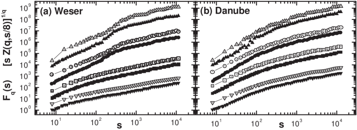
Figure 2: Comparison of the fluctuation functions $F_{q}(s)$ calculated with the multifractal detrended fluctuation analysis (MF-DFA, filled symbols) with the rescaled wavelet transform modulus maxima (WTMM) partition sums $[sZ(q,s/8)]^{1/q}$ (open symbols) as function of time scale $s$ (in days) for (a) the river Weser (Vlotho, Germany, 171y) and (b) the river Danube (Orsova, Romania, 151y). The different symbols indicate different moments, $q=-6$ (triangles up), $q=-2$ (circles), $q=2$ (squares), $q=6$ (triangles down), and the curves are shifted vertically for clarity. The slopes $h(q)$ for large $s$ of both, the MF-DFA curves and the rescaled WTMM curves are equivalent.

In the MF-DFA procedure [8], the moments $F_{q}(s)$ are calculated by (i) integrating the series, (ii) splitting the series into segments of length $s$, (iii) calculating the mean-square deviations $F^{2}(\nu,s)$ from polynomial fits in each segment, (iv) averaging $[F^{2}(\nu,s)]^{q/2}$ over all segments, and (v) taking the $q$th root. In the paper, we have used third order polynomials in the fitting procedure of step (iii) (MF-DFA3), this way eliminating quadratic trends in the data. We consider both, positive and negative moments $F_{q}(s)$ ($q$ ranges from $-10$ to $+10$) and determine them for time scales $s$ between $s=5$ and $s=N/5$, where $N$ is the length of the series. Figure 2 shows the results (filled symbols) for two representative hydrological stations. On large time scales, above a crossover occurring around 30-200 days, we observe a power-law scaling behaviour,

$$F_{q}(s)\sim s^{h(q)},$$ (1)

where the scaling exponent $h(q)$ (the slope in Fig. 2) explicitly depends on the value of $q$. This behaviour represents the presence of multifractality.

In order to test the MF-DFA approach we have applied the well-established WTMM technique, which is also detrending but based on wavelet analysis instead of polynomial fitting procedures. For a full description of the method, we refer to [11, 12]. First, the wavelet-transform $T(n,s^{\prime})={1\over s^{\prime}}\sum_{i=1}^{N}\phi_{i}\,g[(i-n)/s^{\prime}]$ of the departures $\phi_{i}$ is calculated. For the wavelet $g(x)$ we choose the third derivative of a Gaussian here, $g(x)=d^{3}(e^{-x^{2}/2})/dx^{3}$, which is orthogonal to quadratic trends. Now, for a given scale $s^{\prime}$, one determines the positions $n_{i}$ of the local maxima of $|T(n,s^{\prime})|$, so that $|T(n_{i}-1,s^{\prime})|<|T(n_{i},s^{\prime})|\geq|T(n_{i}+1,s^{\prime})|$. Then, one obtains the WTMM partition sum $Z_{q}(s^{\prime})$ by averaging $|T(n_{i},s^{\prime})|^{q}$ for all maxima $n_{i}$. An additional supremum procedure has to be used in the WTMM method in order to keep the dependence of $Z(q,s^{\prime})$ on $s^{\prime}$ monotonous [12]. The expected scaling behaviour is $Z(q,s^{\prime})\sim(s^{\prime})^{\tau(q)}$, where $\tau(q)$ are the Renyi exponents. Since $\tau(q)$ is related to the exponents $h(q)$ by $h(q)=[\tau(q)+1]/q$ [8] we have plotted

$$[sZ(q,s/8)]^{1/q}\sim s^{[\tau(q)+1]/q}\sim s^{h(q)}.$$ (2)

We set $s^{\prime}=s/8$ in the comparison with the MF-DFA results, since the wavelet we employ can be well approximated within a window of size $8s^{\prime}$ (i.e. within 4 standard deviations on both sides), and this window size corresponds to the segment length $s$ in the MF-DFA. Figure 2 shows that both methods yield equivalent results for the $q$ values we considered.

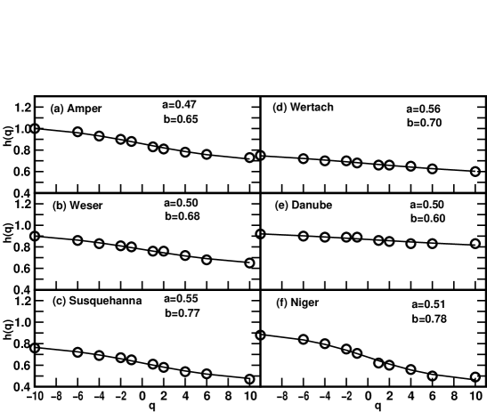
Figure 3: The generalized Hurst exponents $h(q)$ for six representative daily runoff records: (a) Amper in Fürstenfeldbruck, Germany, (b) Weser in Vlotho, Germany, (c) Susquehanna in Harrisburg, USA, (d) Wertach in Biessenhofen, Germany, (e) Danube in Orsova, Romania, and (f) Niger in Koulikoro, Mali. The $h(q)$ values have been determined by straight line fits of $F_{q}(s)$ on large time scales. The error bars of the fits correspond to the size of the symbols. The lines are obtained by fits of the two-parameter binomial model yielding Eq. (3). The resulting model parameters $a$ and $b$ are reported in the figures. All fits are consistent with the data within the error bars (from [13]).

Using the MF-DFA results, we have determined $h(q)$ from Eq. (1) for all runoff records and all precipitation records and for several values of $q$. Since a crossover occurs in $F_{q}(s)$ for time scales in the range of 30-200 days, we considered only sufficiently long time scales (above one year), where the results scale well. Figure 3 shows $h(q)$ for the runoff data, while Fig. 4 shows $h(q)$ for the precipitation data. Together with the results we show least-square fits according to the formula

$$h(q)={1\over q}-{\ln[a^{q}+b^{q}]\over q\ln 2},$$ (3)

which corresponds to $\tau(q)=-\ln[a^{q}+b^{q}]/\ln 2$ and can be obtained from a generalized binomial multifractal model [13], see also [4, 8]. The values of the two parameters $a$ and $b$ are also reported in the figures. The results for all rivers can be fitted surprisingly well with only these two parameters (see Fig. 3). Instead of choosing $a$ and $b$, we could also choose the Hurst exponent $h(1)$ and the persistence exponent $h(2)$. From knowledge of two moments, all the other moments follow.

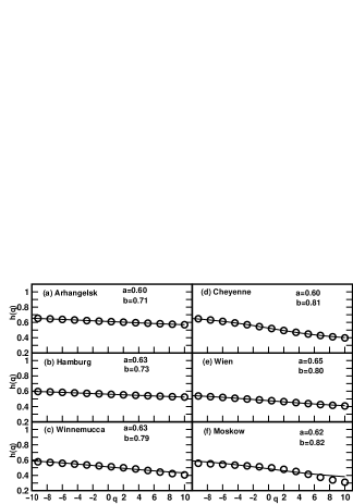
Figure 4: The generalized Hurst exponents $h(q)$ for six representative daily precipitation records: (a) Arhangelsk (Russia), (b) Hamburg (Germany), (c) Winnemucca (USA), (d) Cheyenne (USA), (e) Vienna (Austria), (f) Moskow (Russia), analogous with Fig. 3. While the fits in (a,b,d,e) are consistent with the data within the error bars, significant deviations occur in (c) and – even more drastically – in (f).

This surprising result does not hold for the precipitation records. As can be seen in Figs. 4(c) and 4(f) there are stations where Eq. (3) cannot describe the multifractal scaling behaviour reasonably well. According to Rybski et al., Eq. (3) is appropriate only for about 50 percent of the precipitation records [14].

In the generalized binomial multifractal model, the strength of multifractality is described by the difference of the asymptotical values of $h(q)$, $\Delta\alpha\equiv h(-\infty)-h(\infty)=(\ln b-\ln a)/\ln 2$. We note that this parameter is identical to the width of the singularity spectrum $f(\alpha)$ at $f=0$. Studying 41 river runoff records [13], we have obtained an average $\Delta\alpha=0.49\pm 0.16$, which indicates rather strong multifractality on the long time scales considered. For the precipitation records, on the other hand, the multifractality is weaker. The average is $\Delta\alpha=0.29\pm 0.14$ for 83 records [14].

Our results for $h(q)$ may be compared with the different ansatz $h(q)=1+H^{\prime}-C_{1}(q^{\alpha^{\prime}-1}-1)/(\alpha^{\prime}-1)$ with the three parameters $H^{\prime}$, $C_{1}$, and $\alpha^{\prime}$ (LS ansatz), that has been used by Lovejoy, Schertzer, and coworkers [6, 7] successfully to describe the multifractal behaviour of rainfall and runoff records for $q>0$. A quantitative comparison between both methods is inhibited, since here we considered only long time scales and used detrending methods. We like to note that formula (3) for $h(q)$ is not only valid for positive $q$ values, but also for negative $q$ values. We find it remarkable, that for the runoff records only two parameters were needed to fit the data. For the precipitation data, one needs either three parameters like in the LS ansatz or different schemes.

In summary, we have analyzed long river discharge records and long precipitation records using the multifractal detrended fluctuation analysis (MF-DFA) and the wavelet transform modulus maxima (WTMM) method. We obtained agreement within the error margins and found that the runoff records are characterized by stronger multifractality than the precipitation records. Surprisingly, the type of multifractality occurring in all runoff records is consistent with a modified version of the binomial multifractal model, which supports the idea of a ’universal’ multifractal behaviour of river runoffs suggested by Lovejoy and Schertzer. In contrast, according to [14], several precipitation records seem to require a different description or a three-parameter fit like the LS ansatz. The multifractal exponents can be regarded as ’fingerprints’ for each station. Furthermore, a multifractal generator based on the modified binomial multifractal model can be used to generate surrogate data with specific properties for each runoff record and for some of the precipitation records.

Acknowledgments: We would like to thank the German Science Foundation (DFG), the German Federal Ministry of Education and Research (BMBF), the Israel Science Foundation (ISF), and the Minerva Foundation for financial support. We also would like to thank H. Österle for providing some of the observational data.

References

- [1] H. E. Hurst, Transact. Am. Soc. Civil Eng. 116 (1951) 770.
- [2] H. E. Hurst, R. P. Black, Y. M. Simaika, Long-term storage: An experimental study, (Constable & Co. Ltd., London, 1965).
- [3] B. B. Mandelbrot, J. R. Wallis, Wat. Resour. Res. 5 (1969) 321.
- [4] J. Feder, Fractals, (Plenum Press, New York, 1988).
- [5] C. Matsoukas, S. Islam, I. Rodriguez-Iturbe, J. Geophys. Res. Atmosph. 105 (2000) 29165.
- [6] Y. Tessier, S. Lovejoy, P. Hubert, D. Schertzer, S. Pecknold, J. Geophys. Res. Atmosph. 101 (1996) 26427.
- [7] G. Pandey, S. Lovejoy, D. Schertzer, J. Hydrol. 208 (1998) 62.
- [8] J. W. Kantelhardt, S. A. Zschiegner, E. Koscielny-Bunde, S. Havlin, A. Bunde, H. E. Stanley, Physica A 316 (2002) 87.
- [9] E. Koscielny-Bunde, A. Bunde, S. Havlin, H. E. Roman, Y. Goldreich, H.-J. Schellnhuber, Phys. Rev. Lett. 81 (1998) 729.
- [10] R. O. Weber, P. Talkner, J. Geophys. Res. Atmosph. 106 (2001) 20131.
- [11] J. F. Muzy, E. Bacry, A. Arneodo, Phys. Rev. Lett. 67 (1991) 3515.
- [12] A. Arneodo, B. Audit, N. Decoster, J.-F. Muzy, C. Vaillant, Wavelet Based Multifractal Formalism: Applications to DNA Sequences, Satellite Images of the Cloud Structure, and Stock Market Data, in: A. Bunde, J. Kropp, H.-J. Schellnhuber, The science of disaster: climate disruptions, market crashes, and heart attacks, (Springer, Berlin, 2002), pp. 27-102.
- [13] E. Koscielny-Bunde, J. W. Kantelhardt, P. Braun, A. Bunde, S. Havlin, submitted to Wat. Resour. Res. (2003).
- [14] D. Rybski et al., in preparation (2003).