Long-term persistence and multifractality of river runoff records: Detrended fluctuation studies

Abstract

We study temporal correlations and multifractal properties of long river discharge records from 41 hydrological stations around the globe. To detect long-term correlations and multifractal behaviour in the presence of trends, we apply several recently developed methods [detrended fluctuation analysis (DFA), wavelet analysis, and multifractal DFA] that can systematically detect and overcome nonstationarities in the data at all time scales. We find that above some crossover time that usually is several weeks, the daily runoffs are long-term correlated, being characterized by a correlation function $C(s)$ that decays as $C(s)\sim s^{-\gamma}$. The exponent $\gamma$ varies from river to river in a wide range between 0.1 and 0.9. The power-law decay of $C(s)$ corresponds to a power-law increase of the related fluctuation function $F_{2}(s)\sim s^{H}$ where $H=1-\gamma/2$. We also find that in most records, for large times, weak multifractality occurs. The Renyi exponent $\tau(q)$ for $q$ between $-10$ and $+10$ can be fitted to the remarkably simple form $\tau(q)=-\ln(a^{q}+b^{q})/\ln 2$, with solely two parameters $a$ and $b$ between 0 and 1 with $a+b\geq 1$. This type of multifractality is obtained from a generalization of the multiplicative cascade model.

, , , , and

1 Introduction

The analysis of river flows has a long history. Already more than half a century ago Hurst found by means of his $R/S$ analysis that annual runoff records from various rivers (including the Nile river) exhibit ”long-range statistical dependencies” (Hurst, 1951), indicating that the fluctuations in water storage and runoff processes are self-similar over a wide range of time scales, with no single characteristic scale. Hurst’s finding is now recognized as the first example for self-affine fractal behaviour in empirical time series, see e.g. Feder (1988). In the 1960s, the ”Hurst phenomenon” was investigated on a broader empirical basis for many other natural phenomena (Hurst et al., 1965; Mandelbrot and Wallis, 1969).

The scaling of the fluctuations with time is reflected by the scaling of the power spectrum $E(f)$ with frequency $f$, $E(f)\sim f^{-\beta}$. For stationary time series the exponent $\beta$ is related to the decay of the corresponding autocorrelation function $C(s)$ of the runoffs (see Eq. (1)). For $\beta$ between 0 and 1, $C(s)$ decays by a power law, $C(s)\sim s^{-\gamma}$, with $\gamma=1-\beta$ being restricted to the interval between 0 and 1. In this case, the mean correlation time diverges, and the system is regarded as long-term correlated. For $\beta=0$, the runoff data are uncorrelated on large time scales (”white noise”). The exponents $\beta$ and $\gamma$ can also be determined from a fluctuation analysis, where the departures from the mean daily runoffs are considered as increments of a random walk process. If the runoffs are uncorrelated, the fluctuation function $F_{2}(s)$, which is equivalent to the root-mean-square displacement of the random walk, increases as the square root of the time scale $s$, $F_{2}(s)\sim\sqrt{s}$. For long-term correlated data, the random walk becomes anomalous, and $F_{2}(s)\sim s^{H}$. The fluctuation exponent $H$ is related to the exponents $\beta$ and $\gamma$ via $\beta=1-\gamma=2H-1$. For monofractal data, $H$ is identical to the classical Hurst exponent. Recently, many studies using these kinds of methods have dealt with scaling properties of hydrological records and the underlying statistics, see e. g. Lovejoy and Schertzer (1991); Turcotte and Greene (1993); Gupta et al. (1994); Tessier et al. (1996); Davis et al. (1996); Rodriguez-Iturbe and Rinaldo (1997); Pandey et al. (1998); Matsoukas et al. (2000); Montanari et al. (2000); Peters et al. (2002); Livina et al. (2003a, b).

However, the conventional methods discussed above may fail when trends are present in the system. Trends are systematic deviations from the average runoff that are caused by external processes, e.g. the construction of a water regulation device, the seasonal cycle, or a changing climate (e.g. global warming). Monotonous trends may lead to an overestimation of the Hurst exponent and thus to an underestimation of $\gamma$. It is even possible that uncorrelated data, under the influence of a trend, look like long-term correlated ones when using the above analysis methods. In addition, long-term correlated data cannot simply be detrended by the common technique of moving averages, since this method destroys the correlations on long time scales (above the window size used). Furthermore, it is difficult to distinguish trends from long-term correlations, because stationary long-term correlated time series exhibit persistent behaviour and a tendency to stay close to the momentary value. This causes positive or negative deviations from the average value for long periods of time that might look like a trend.

In the last years, several methods such as wavelet techniques (WT) and detrended fluctuation analysis (DFA), have been developed that are able to determine long-term correlations in the presence of trends. For details and applications of the methods to a large number of meteorological, climatological and biological records we refer to Peng et al. (1994); Taqqu et al. (1995); Bunde et al. (2000); Kantelhardt et al. (2001); Arneodo et al. (2002); Bunde et al. (2002). The methods, described in Section 2, consider fluctuations in the cumulated runoffs (often called the ”profile” or ”landscape” of the record). They differ in the way the fluctuations are determined and in the type of polynomial trend that is eliminated in each time window of size $s$.

In this paper, we apply these detrending methods to study the scaling of the fluctuations $F_{2}(s)$ of river flows with time $s$. We focus on 23 runoff records from international river stations spread around the globe and compare the results with those of 18 river stations from southern Germany. We find that above some crossover time (typically several weeks) $F_{2}(s)$ scales as $s^{H}$ with $H$ varying from river to river between 0.55 and 0.95 in a nonuniversal manner independent of the size of the basin. The lowest exponent $H=0.55$ was obtained for rivers on permafrost ground. Our finding is not consistent with the hypothesis that the scaling is universal with an exponent close to 0.75 (Hurst et al., 1965; Feder, 1988) with the same power law being applicable for all time scales from minutes till centuries.

The above detrending approaches, however, are not sufficient to fully characterize the complex dynamics of river flows, since they exclusively focus on the variance which can be regarded as the second moment $F_{2}(s)$ of the full distribution of the fluctuations. Note that the Hurst method actually focuses on the first moment $F_{1}(s)$. To further characterize a hydrological record, we extend the study to include all moments $F_{q}(s)$. A detailed description of the method, which is a multifractal generalization of the detrended fluctuation analysis (Kantelhardt et al., 2002) and equivalent to the Wavelet Transform Modulus Maxima (WTMM) method (Arneodo et al., 2002), is given in Section 3. Our approach differs from the multifractal approach introduced into hydrology by Lovejoy and Schertzer (see e.g. Schertzer and Lovejoy (1987); Lovejoy and Schertzer (1991); Lavallee et al. (1993); Pandey et al. (1998)) that was based on the concept of structure functions (Frisch and Parisi, 1985) and on the assumption of the existence of a universal cascade model. Here we perform the multifractal analysis by studying how the different moments of the fluctuations $F_{q}(s)$ scale with time $s$, see also Rodriguez-Iturbe and Rinaldo (1997). We find that at large time scales, $F_{q}(s)$ scales as $s^{h(q)}$, and a simple functional form with two parameters ($a$ and $b$), $h(q)=(1/q)-[\ln(a^{q}+b^{q})]/[q\ln(2)]$ describes the scaling exponent $h(q)$ of all moments. On small time scales, however, a stronger multifractality is observed that may be partly related to the seasonal trend. The mean position of the crossover between the two regimes is of the order of weeks and increases with $q$.

2 Correlation Analysis

Consider a record of daily water runoff values $W_{i}$ measured at a certain hydrological station. The index $i$ counts the days in the record, $i=1$,2,…,$N$. To eliminate the periodic seasonal trends, we concentrate on the departures $\phi_{i}=W_{i}-\overline{W_{i}}$ from the mean daily runoff $\overline{W_{i}}$. $\overline{W_{i}}$ is calculated for each calendar date $i$ (e.g. April 1^st) by averaging over all years in the runoff series. In addition, we checked that our actual results remained unchanged when also seasonal trends in the variance have been eliminated by analysing $\phi^{\prime}_{i}=(W_{i}-\overline{W_{i}})/(\overline{W^{2}_{i}}-\overline{W_{i}}^{2})^{1/2}$ instead of $\phi_{i}$.

The runoff autocorrelation function $C(s)$ describes, how the persistence decays in time. If the $\phi_{i}$ are uncorrelated, $C(s)$ is zero for all $s$. If correlations exist only up to a certain number of days $s_{\times}$, the correlation function will vanish above $s_{\times}$. For long-term correlations, $C(s)$ decays by a power-law

$$C(s)=\langle\phi_{i}\phi_{i+s}\rangle\sim s^{-\gamma},\qquad 0<\gamma<1,$$ (1)

where the average $\langle\ldots\rangle$ is over all pairs with the same time lag $s$. For large values of $s$, a direct calculation of $C(s)$ is hindered by the level of noise present in the finite hydrological records, and by nonstationarities in the data. There are several alternative methods for calculating the correlation function in the presence of long-term correlations, which we describe in the following sections.

2.1 Power Spectrum Analysis

If the time series is stationary, we can apply standard spectral analysis techniques and calculate the power spectrum $E(f)$ of the time series $W_{i}$ as a function of the frequency $f$. For long-term correlated data, we have $E(f)\sim f^{-\beta},$ where $\beta$ is related to the correlation exponent $\gamma$ by $\beta=1-\gamma$. This relation can be derived from the Wiener-Khinchin theorem. If, instead of $W_{i}$ the integrated runoff time series $z_{n}=\sum_{i=1}^{n}\phi_{i}$ is Fourier transformed, the resulting power spectrum scales as $\tilde{E}(f)\sim f^{-2-\beta}$.

2.2 Standard Fluctuation Analysis (FA)

In the standard fluctuation analysis, we consider the “runoff profile”

$$z_{n}=\sum_{i=1}^{n}\phi_{i},\qquad n=1,2,\ldots,N,$$ (2)

and study how the fluctuations of the profile, in a given time window of size $s$, increase with $s$. We can consider the profile $z_{n}$ as the position of a random walker on a linear chain after $n$ steps. The random walker starts at the origin and performs, in the $i$th step, a jump of length $\phi_{i}$ to the right, if $\phi_{i}$ is positive, and to the left, if $\phi_{i}$ is negative.

To find how the square-fluctuations of the profile scale with $s$, we first divide each record of $N$ elements into $N_{s}={\rm int}(N/s)$ nonoverlapping segments of size $s$ starting from the beginning and $N_{s}$ nonoverlapping segments of size $s$ starting from the end of the considered runoff series. Then we determine the fluctuations in each segment $\nu$.

In the standard fluctuation analysis, we obtain the fluctuations just from the values of the profile at both endpoints of each segment $\nu$, $F^{2}(\nu,s)=[z_{\nu s}-z_{(\nu-1)s}]^{2}$, and average $F^{2}(\nu,s)$ over the $2N_{s}$ subsequences to obtain the mean fluctuation $F_{2}(s)$,

$$F_{2}(s)\equiv\left\{{1\over 2N_{s}}\sum_{\nu=1}^{2N_{s}}F^{2}(\nu,s)\right\}^{1/2}.$$ (3)

By definition, $F_{2}(s)$ can be viewed as the root-mean-square displacement of the random walker on the chain, after $s$ steps. For uncorrelated $\phi_{i}$ values, we obtain Fick’s diffusion law $F_{2}(s)\sim s^{1/2}$. For the relevant case of long-term correlations, where $C(s)$ follows the power-law behaviour of Eq. (1), $F_{2}(s)$ increases by a power law (see, e.g., Bunde et al. (2002)),

$$F_{2}(s)\sim s^{H},$$ (4)

where the fluctuation exponent $H$ is related to the correlation exponent $\gamma$ and the power-spectrum exponent $\beta$ by

$$H=1-\gamma/2=(1+\beta)/2.$$ (5)

For power-law correlations decaying faster than $1/s$, we have $H=1/2$ for large $s$ values, like for uncorrelated data.

We like to note that the standard fluctuation analysis is somewhat similar to the rescaled range analysis introduced by Hurst (for a review see, e. g., Feder (1988)), except that it focusses on the second moment $F_{2}(s)$ while Hurst considered the first moment $F_{1}(s)$. For monofractal data, $H$ is identical to the Hurst exponent.

2.3 The Detrended Fluctuation Analysis (DFA)

There are different orders of DFA that are distinguished by the way the trends in the data are eliminated. In lowest order (DFA1) we determine, for each segment $\nu$, the best linear fit of the profile, and identify the fluctuations by the variance $F^{2}(\nu,s)$ of the profile from this straight line. This way, we eliminate the influence of possible linear trends on scales larger than the segment. Note that linear trends in the profile correspond to patch-like trends in the original record. DFA1 has been proposed originally by Peng et al. (1994) when analyzing correlations in DNA. It can be generalized straightforwardly to eliminate higher order trends (Bunde et al., 2000; Kantelhardt et al., 2001).

In second order DFA (DFA2) one calculates the variances $F^{2}(\nu,s)$ of the profile from best quadratic fits of the profile, this way eliminating the influence of possible linear and parabolic trends on scales larger than the segment considered. In general, in $n$th-order DFA, we calculate the variances of the profile from the best $n$th-order polynomial fit, this way eliminating the influence of possible $(n-1)$th-order trends on scales larger than the segment size.

Explicitly, we calculate the best polynomial fit $y_{\nu}(i)$ of the profile in each of the $2N_{s}$ segments $\nu$ and determine the variance

$$F^{2}(\nu,s)\equiv{1\over s}\sum_{i=1}^{s}\left[z_{(\nu-1)s+i}-y_{\nu}(i)\right]^{2}.$$ (6)

Then we employ Eq. (3) to determine the mean fluctuation $F_{2}(s)$.

Since FA and the various stages of the DFA have different detrending capabilities, a comparison of the fluctuation functions obtained by FA and DFA$n$ can yield insight into both long-term correlations and types of trends. This cannot be achieved by the conventional methods, like the spectral analysis.

2.4 Wavelet Transform (WT)

The wavelet methods we employ here are based on the determination of the mean values $\overline{z}_{\nu}(s)$ of the profile in each segment $\nu$ (of length $s$), and the calculation of the fluctuations between neighbouring segments. The different order techniques we have used in analyzing runoff fluctuations differ in the way the fluctuations between the average profiles are treated and possible nonstationarities are eliminated. The first-, second- and third-order wavelet method are described below.

(i) In the first-order wavelet method (WT1), one simply determines the fluctuations from the first derivative $F^{2}(\nu,s)=[\overline{z}_{\nu}(s)-\overline{z}_{\nu+1}(s)]^{2}$. WT1 corresponds to FA where constant trends in the profile of a hydrological station are eliminated, while linear trends are not eliminated.

(ii) In the second-order wavelet method (WT2), one determines the fluctuations from the second derivative $F^{2}(\nu,s)=[\overline{z}_{\nu}(s)-2\overline{z}_{\nu+1}(s)+\overline{z}_{\nu+2}(s)]^{2}$. So, if the profile consists of a trend term linear in $s$ and a fluctuating term, the trend term is eliminated. Regarding trend-elimination, WT2 corresponds to DFA1.

(iii) In the third-order wavelet method (WT3), one determines the fluctuations from the third derivative $F^{2}(\nu,s)=[\overline{z}_{\nu}(s)-3\overline{z}_{\nu+1}(s)+3\overline{z}_{\nu+2}(s)-\overline{z}_{\nu+3}(s)]^{2}$. By definition, WT3 eliminates linear and parabolic trend terms in the profile. In general, in WT$n$ we determine the fluctuations from the $n$th derivative, this way eliminating trends described by $(n-1)$st-order polynomials in the data.

Methods (i-iii) are called wavelet methods, since they can be interpreted as transforming the profile by discrete wavelets representing first-, second- and third-order cumulative derivatives of the profile. The first-order wavelets are known in the literature as Haar wavelets. One can also use different shapes of the wavelets (e.g. Gaussian wavelets with width $s$), which have been used by Arneodo et al. (2002) to study, for example, long-range correlations in DNA. Since the various stages of the wavelet methods WT1, WT2, WT3, etc. have different detrending capabilities, a comparison of their fluctuation functions can yield insight into both long-term correlations and types of trends.

At the end of this section, before describing the results of the FA, DFA, and WT analysis, we note that for very large $s$ values, $s>N/4$ for DFA and $s>N/10$ for FA and WT, the fluctuation function becomes inaccurate due to statistical errors. The difference in the statistics is due to the fact that the number of independent segments of length $s$ is larger in DFA than in WT, and the fluctuations in FA are larger than in DFA. Hence, in the analysis we will concentrate on $s$ values lower than $s_{\rm max}=N/4$ for DFA and $s_{\rm max}=N/10$ for FA and WT. When determining the scaling exponents $H$ using Eq. (4), we manually chose an appropriate (shorter) fitting range of typically two orders of magnitude.

2.5 Results

Figure 1: (a) The fluctuation functions $F_{2}(s)$ versus time scale $s$ obtained from FA and DFA1-DFA5 in double logarithmic plots for daily runoff departures $\phi_{i}=W_{i}-\overline{W_{i}}$ from the mean daily runoff $\overline{W_{i}}$ for the river Weser, measured from 1823 till 1993 by the hydrological station Vlotho in Germany. (b) The analog curves to (a) when the $\phi_{i}$ are randomly shuffled.

In our study we analyzed 41 runoff records, 18 of them are from the southern part of Germany, and the rest is from North and South America, Africa, Australia, Asia and Europe (see Table 1). We begin the analysis with the runoff record for the river Weser in the northern part of Germany, which has the longest record (171 years) in this study. Figure 1(a) shows the fluctuation functions $F_{2}(s)$ obtained from FA and DFA1-DFA5. In the log-log plot, the curves are approximately straight lines for $s$ above 30 days, with a slope $H\approx 0.75$. This result for the Weser suggests that there exists long-term persistence expressed by the power-law decay of the correlation function, with an exponent $\gamma\approx 0.5$ [see Eq. (4)].

To show that the slope $H\approx 0.75$ is due to long-term correlations and not due to a broad probability distribution (Joseph- versus Noah-Phenomenon, see Mandelbrot and Wallis (1968)), we have eliminated the correlations by randomly shuffling the $\phi_{i}$. This shuffling has no effect on the probability distribution function of $\phi_{i}$. Figure 1(b) shows $F_{2}(s)$ for the shuffled data. We obtain $H=1/2$, showing that the exponent $H\approx 0.75$ is due to long-term correlations.

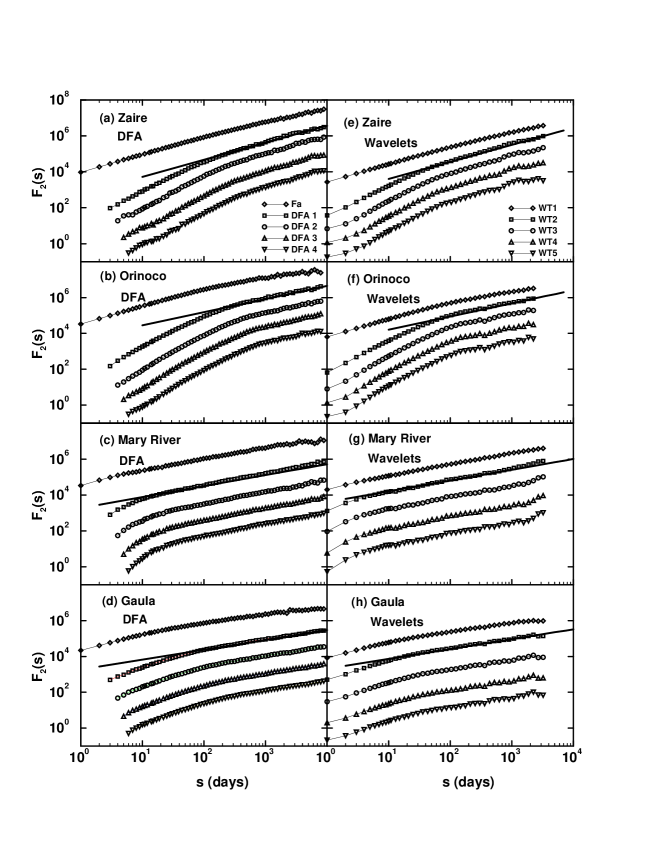
Figure 2: The fluctuation functions $F_{2}(s)$ versus time scale $s$ obtained from FA and DFA1-DFA4 in double logarithmic plots for four additional representative hydrological stations: (a) the Zaire in Kinshasa, Zaire, (b) the Orinoco in Puente Angostura, Venezuela, (c) the Mary River in Miva, Australia, and (d) the Gaula River in Haga Bru, Norway. (e-h) the fluctuation functions $F_{2}(s)$ obtained for the same rivers as in (a-d), from first to fifth order wavelet analysis (WT1-WT5). The straight lines are best linear fits to the DFA1 and the WT2 results on large time scales.

To show that the slope $H\approx 0.75$ is not an artefact of the seasonal dependence of the variance and skew, we also considered records where $\phi_{i}$ was divided by the variance of each calendary day and applied further detrending techniques that take into account the skew (Livina et al., 2003b). In both cases, we found no change in the scaling behaviour for large times (see also Sect. 3.4). This can be understood easily, since kinds of seasonal trends cannot effect the fluctuation behaviour on time scales well above one year. It is likely, however, that the seasonal dependencies of the variance and possibly also of the skew contribute to the behaviour at small times, where the slope $H$ is much larger than 0.75 in most cases (see also Sect. 3.4, where a seasonal trend in the variance is indeed used for modelling the crossover).

Figure 2 shows the fluctuation functions $F_{2}(s)$ of 4 more rivers, from Africa, South America, Australia, and Europe. The panels on the left-hand side show the FA and DFA1-4 curves, while the panels on the right-hand side show the results from the analogous wavelet analysis WT1-WT5. Most curves show a crossover at small time scales; a similar crossover has been reported by Tessier et al. (1996) for small French rivers without artificial dams or reservoirs. Above the crossover time, the fluctuation functions (from DFA1-4 and WT2-5) show power-law behaviour, with exponents $H\simeq 0.95$ for the Zaire, $H\simeq 0.73$ for the Orinoco, $H\simeq 0.60$ for the Mary river, and $H\simeq 0.55$ for the Gaula river.

Accordingly, there is no universal scaling behaviour since the long-term exponents vary strongly from river to river and reflect the fact that there exist different mechanisms for floods where each may induce different scaling. This is in contrast to climate data, where universal long-term persistence of temperature records at land stations was observed (Koscielny-Bunde et al., 1998; Talkner and Weber, 2000; Weber and Talkner, 2001; Eichner et al., 2003).

The Mary river in Australia is rather dry in the summer and the Gaula river in Norway is frozen in the winter. For the Mary river, the long-term exponent $H\simeq 0.60$ is well below the average value. For the Gaula river, the long-term correlations are not pronounced ($H=0.55$) and even hard to distinguish from the uncorrelated case $H=0.5$. We obtained similar results for the other two ”frozen” rivers (Tana from Norway and Dvina from Russia) that we analysed. For interpreting this distinguished behaviour of the frozen rivers we like to note that on permafrost ground the lateral inflow (and hence the indirect contribution of the water storage in the catchment basin) contributes to the runoffs in a different way than on normal ground, see also Gupta and Dawdy [1995]. Our results (based on 3 rivers only) suggest that the contribution of snow melting leads to less correlated runoffs than the contribution of rainfall, but more comprehensive studies will be needed to confirm this interesting result.

Figure 3(a) and Table 1 summarize our results for $H$. One can see clearly that the exponents $H$ do not depend systematically on the basin area $A$. This is in line with the conclusions of Gupta et al. (1994) for the flood peaks, where a systematic dependence on $A$ could also not be found.

Table 1: Table of investigated international river basins (data from Global Runoff Data Center (GRDC), Koblenz, Germany) and investigated South German river basins. We list the river and station name, the duration of the investigated daily record, the size of the basin area, and the results of our analysis, $H=h(2)$, the multifractal quantities $a$, $b$, and $\Delta\alpha$.

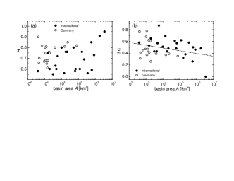
Figure 3: (a) Long-term fluctuation exponents $H$ and (b) widths $\Delta\alpha$ of the $f(\alpha)$ spectra for all international records (full symbols) and all records from south Germany (open symbols) that we analyzed, as a function of the basin area $A$. Each symbol represents the result for one hydrological station. The dashed line in (b) is a linear fit to the data.

There is also no pronounced regional dependence: the rivers within a localized area (such as South Germany) tend to have nearly the same range of exponents as the international rivers. The three ”frozen” rivers in our study have the lowest values of $H$. As can be seen in the figure, the exponents spread from 0.55 to 0.95. Since the correlation exponent $\gamma$ is related to $H$ by $\gamma=2-2H$, the exponent $\gamma$ spreads from almost 0 to almost 1, covering the whole range from very weak to very strong correlations.

3 Multifractal Analysis

3.1 Method

For a further characterization of hydrological records it is meaningful to extend Eq. (3) by considering the more general fluctuation functions (Barabasi and Vicsek (1991), see also Davis et al. (1996)),

$$F_{q}(s)=\left\{{1\over 2N_{s}}\sum_{\nu=1}^{2N_{s}}|z_{\nu s}-z_{(\nu-1)s}|^{q}\right\}^{1/q}.$$ (7)

where the variable $q$ can take any real value except zero. For $q=2$, the standard fluctuation analysis is retrieved. The question is, how the fluctuation functions depend on $q$ and how this dependence is related to multifractal features of the record.

In general, the multifractal approach is introduced by the partition function

$$Z_{q}(s)\equiv\sum_{\nu=1}^{N_{s}}|z_{\nu s}-z_{(\nu-1)s}|^{q}\sim s^{\tau(q)},$$ (8)

where $\tau(q)$ is the Renyi scaling exponent. A record is called ’monofractal’, when $\tau(q)$ depends linearly on $q$; otherwise it is called multifractal.

It is easy to verify that $Z_{q}(s)$ is related to $F_{q}(s)$ by

$$F_{q}(s)=\left\{{1\over N_{s}}Z_{q}(s)\right\}^{1/q}.$$ (9)

Accordingly, Eq. (8) implies

$$F_{q}(s)\sim s^{h(q)},$$ (10)

where

$$h(q)=[\tau(q)+1]/q.$$ (11)

Thus, $h(q)$ defined in Eq. (10) is directly related to the classical multifractal scaling exponents $\tau(q)$.

In general, the exponent $h(q)$ may depend on $q$. Since for stationary records, $h(1)$ is identical to the well-known Hurst exponent (see e. g. Feder (1988)), we will call the function $h(q)$ the generalized Hurst exponent. For monofractal self-affine time series, $h(q)$ is independent of $q$, since the scaling behaviour of the variances $F^{2}(\nu,s)$ is identical for all segments $\nu$, and the averaging procedure in Eq. (7) will give just this identical scaling behaviour for all values of $q$. If small and large fluctuations scale differently, there will be a significant dependence of $h(q)$ on $q$: If we consider positive values of $q$, the segments $\nu$ with large variance $F^{2}(\nu,s)$ (i. e. large deviations from the corresponding fit) will dominate the average $F_{q}(s)$. Thus, for positive values of $q$, $h(q)$ describes the scaling behaviour of the segments with large fluctuations. Usually the large fluctuations are characterized by a smaller scaling exponent $h(q)$ for multifractal series. On the contrary, for negative values of $q$, the segments $\nu$ with small variance $F^{2}(\nu,s)$ will dominate the average $F_{q}(s)$. Hence, for negative values of $q$, $h(q)$ describes the scaling behaviour of the segments with small fluctuations, which are usually characterized by a larger scaling exponent.

In the hydrological literature (Rodriguez-Iturbe and Rinaldo, 1997; Lavallee et al., 1993) one often considers the generalized mass variogram $C_{q}(\lambda)$ (see also Davis et al. (1996)),

$$C_{q}(\lambda)\equiv\langle|z_{i+\lambda}-z_{i}|^{q}\rangle\sim\lambda^{K(q)}.$$ (12)

Comparing Eqs. (7), (10), and (12) one can verify easily that $K(q)$ and $h(q)$ are related by

$$h(q)=K(q)/q.$$ (13)

Another way to characterize a multifractal series is the singularity spectrum $f(\alpha)$, that is related to $\tau(q)$ via a Legendre transform (e.g. Feder (1988); Rodriguez-Iturbe and Rinaldo (1997)),

$$\alpha={d\tau(q)\over dq}\quad{\rm and}\quad f(\alpha)=q\alpha-\tau(q).$$ (14)

Here, $\alpha$ is the singularity strength or Hölder exponent, while $f(\alpha)$ denotes the dimension of the subset of the series that is characterized by $\alpha$. Using Eq. (11), we can directly relate $\alpha$ and $f(\alpha)$ to $h(q)$,

$$\alpha=h(q)+q{dh(q)\over dq}\quad{\rm and}\quad f(\alpha)=q[\alpha-h(q)]+1.$$ (15)

The strength of the multifractality of a time series can be characterized by the difference between the maximum and minimum values of $\alpha$, $\alpha_{\rm max}-\alpha_{\rm min}$. When $q{dh(q)\over dq}$ approaches zero for $q$ approaching $\pm\infty$, then $\Delta\alpha=\alpha_{\rm max}-\alpha_{\rm min}$ is simply given by $\Delta\alpha=h(-\infty)-h(\infty)$.

The multifractal analysis described above is a straightforward generalization of the fluctuation analysis and therefore has the same problems: (i) monotonous trends in the record may lead to spurious results for the fluctuation exponent $h(q)$ which in turn leads to spurious results for the correlation exponent $\gamma$, and (ii) nonstationary behaviour characterized by exponents $h(q)>1$ cannot be detected by the simple method since the method cannot distinguish between exponents $>1$, and always will yield $F_{2}(s)\sim s$ in this case (see above). To overcome these drawbacks the multifractal detrended fluctuation analysis (MF-DFA) has been introduced recently (Kantelhardt et al. (2002), see also Koscielny-Bunde et al. (1998); Weber and Talkner (2001)). According to Kantelhardt et al. (2002, 2003), the method is as accurate as the wavelet methods. Thus, we have used MF-DFA for the multifractal analysis here. In the MF-DFA, one starts with the DFA-fluctuations $F_{\nu}^{2}(s)$ as obtained in Eq. (6). Then, we define in close analogy to Eqs. (3) and (7) the generalized fluctuation function,

$$F_{q}(s)\equiv\left\{{1\over 2N_{s}}\sum_{\nu=1}^{2N_{s}}\left[F^{2}(\nu,s)\right]^{q/2}\right\}^{1/q}.$$ (16)

Again, we can distinguish MF-DFA1, MF-DFA2, etc., according to the order of the polynomial fits involved.

Figure 4: The multifractal fluctuation functions $F_{q}(s)$ versus time scale $s$ obtained from multifractal DFA4 for two representative hydrological stations: (a) river Weser in Vlotho, Germany and (b) river Danube in Orsova, Romania. The curves correspond to different values of $q$, $q=-10$, -6, -4, -2, -1, -0.2, 0.2, 1, 2, 4, 6, 10 (from the top to the bottom) and are shifted vertically for clarity.

3.2 Multifractal Scaling Plots

We have performed a large scale multifractal analysis on all 41 rivers. We found that MF-DFA2-5 yield similar results for the fluctuation function $F_{q}(s)$. We have also cross checked the results using the Wavelet Transform Modulus Maxima (WTMM) method (Arneodo et al., 2002), and always find agreement within the error bars (Kantelhardt et al., 2003). Therefore, we present here only the results of MF-DFA4. Figure 4(a,b) shows two representative examples for the fluctuation functions $F_{q}(s)$, for (a) the Weser river and (b) the Danube river. The standard fluctuation function $F_{2}(s)$ is plotted in full symbols. The crossover in $F_{2}(s)$ that was discussed in Sect. 2.5 can be also seen in the other moments. The position of the crossover increases monotonously with decreasing $q$ and the crossover becomes more pronounced. We are only interested in the asymptotic behaviour of $F_{q}(s)$ at large times $s$. One can see clearly that above the crossover, the $F_{q}(s)$ functions are straight lines in the double logarithmic plot, and the slopes increase slightly when going from high positive moments towards high negative moments (from the bottom to the top). For the Weser, for example, the slope changes from 0.65 for $q=10$ to 0.9 for $q=-10$ (see also Fig. 6(b)). The monotonous increase of the slopes, $h(q)$, is the signature of multifractality.

Figure 5: The multifractal fluctuation functions $F_{q}(s)$ obtained from multifractal DFA4 for four additional hydrological stations: (a) Amper in Fürstenfeldbruck, Germany, (b) Wertach in Biessenhofen, Germany, (c) Susquehanna in Harrisburg, USA, (d) Niger in Koulikoro, Mali. The $q$-values are identical to those used in Fig. 4.

When the data are shuffled (see Figs. 4(c,d)), all functions $F_{q}(s)$ increase asymptomatically as $F_{q}(s)\,\sim\,s^{1/2}$. This indicates that the multifractality vanishes under shuffling. Accordingly the observed multifractality originates in the long-term correlations of the record and is not caused by singularities in the distribution of the daily runoffs (see also Mandelbrot and Wallis (1968)). A reshuffling-resistent multifractality would indicate a ’statistical’ type of non-linearity (Sivapalan et al., 2002). We obtain similar patterns for all rivers. Figure 5 shows four more examples; Figs. 5(a,b) are for two rivers (Amper and Wertach) from southern Germany, while Figs. 5(c,d) are for Niger and Susquehama (Koulikoro, Mali and Harrisburg, USA).

From the asymptotic slopes of the curves in Figs. 4(a,b) and 5(a-d), we obtain the generalized Hurst-exponents $h(q)$, which are plotted in Fig. 6 (circles). One can see that in the whole $q$-range the exponents can be fitted well by the formula

$$h(q)={1\over q}-{\ln[a^{q}+b^{q}]\over q\ln 2},$$ (17)

or

$$K(q)=1+\tau(q)=1-{\ln[a^{q}+b^{q}]\over\ln 2}.$$ (18)

The formula can be derived from a modification of the multiplicative cascade model that we describe in Sect. 3.3. Here we use the formula only to show that the infinite number of exponents $h(q)$ can be described by only two independent parameters, $a$ and $b$. These two parameters can then be regarded as multifractal finger print for a considered river. This is particularly important when checking models for river flows. Again, we like to emphasize, that these parameters have been obtained from the asymptotic part of the generalized fluctuation function, and are therefore not affected by seasonal dependencies.

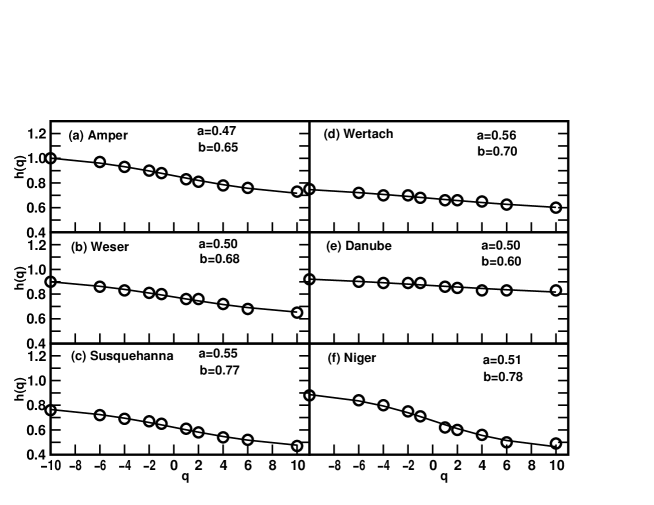
Figure 6: The generalized Hurst exponents $h(q)$ for the six representative daily runoff records analyzed in Figs. 4 and 5: (a) Amper in Fürstenfeldbruck, Germany, (b) Weser in Vlotho, Germany, (c) Susquehanna in Harrisburg, USA, (d) Wertach in Biessenhofen, Germany, (e) Danube in Orsova, Romania, and (f) Niger in Koulikoro, Mali. The $h(q)$ values have been determined by straight line fits of $F_{q}(s)$ on large time scales. The error bars of the fits correspond to the size of the symbols.

We have fitted the $h(q)$ spectra in the range $-10\leq q\leq 10$ for all 41 runoff series by Eq. (17). Representative examples are shown in Fig. 6. The continuous lines in Fig. 6 are obtained by best fits of $h(q)$ (obtained from Figs. 4 and 5 as described above) by Eq. (17). The respective parameters $a$ and $b$ are listed inside the panels of each figure. Our results for the 41 rivers are shown in Table 1. It is remarkable that in each single case, the $q$ dependence of $h(q)$ for positive and negative values of $q$ can be characterized well by the two parameters, and all fits remain within the error bars of the $h(q)$ values.

From $h(q)$ we obtain $\tau(q)$ (Eq. (11)) and the singularity spectrum $f(\alpha)$ (Eq. (15)). Figure 7 shows two typical examples for the Danube and the Niger. The width of $f(\alpha)$ taken at $f=0$ characterizes the strength of the multifractality. Since both widths are very different, the strength of the multifractality of river runoffs appears to be not universal.

Figure 7: The multifractal spectra $f(\alpha)$ for two representative runoff records (a) the Danube in Orsova, Romania and (b) Niger in Koulikoro, Mali.

In order to characterize and to compare the strength of the multifractality for several time series we use as a parameter the width of the singularity spectrum $f(\alpha)$ [see Eqs. (14) and (15)] at $f=0$, which corresponds to the difference of the maximum and the minimum value of $\alpha$. In the multiplicative cascade model, this parameter is given by

$$\Delta\alpha={\ln a-\ln b\over\ln 2}.$$ (19)

The distribution of the $\Delta\alpha$ values we obtained from Eq. (19) is shown in Fig. 3(b), where we plot $\Delta\alpha$ versus the basin area. The figure shows that there are rivers with quite strong multifractal fluctuations, i.e. large $\Delta\alpha$, and one with almost vanishing multifractality, i.e. $\Delta\alpha\approx 0$. Two observation can be made from the figure: (1) There is no pronounced difference between the width of the distribution of the multifractality strength for the runoffs within the local area of southern Germany (open symbols in Fig. 3(b)) and for the international runoff records from all rivers around the globe (full symbols). In fact, without rivers Zaire and Grand River the widths would be the same. (2) There is a tendency towards smaller multifractality strengths at larger basin areas. This means that the river flows become less nonlinear with increasing basin area. We consider this as possible indication of river regulations that are more pronounced for large river basins.

Our results for $K(q)=1+\tau(q)$ (see Eq. (18) and Table 1) may be compared with the functional form

$$K(q)=(H^{\prime}+1)q-{C_{1}\over\alpha^{\prime}-1}(q^{\alpha^{\prime}}-q)\qquad q\geq 0$$ (20)

with the three parameters $H^{\prime}$, $C_{1}$, and $\alpha^{\prime}$, that have been used by Lovejoy, Schertzer, and coworkers (Schertzer and Lovejoy, 1987; Lovejoy and Schertzer, 1991; Lavallee et al., 1993; Tessier et al., 1996; Pandey et al., 1998) successfully to describe the multifractal behaviour of rainfall and runoff records. The definition of $K(q)$ we used in this paper is taken from Rodriguez-Iturbe and Rinaldo (1997) and differs slightly from their definition. We like to note that Eq. (18) for $K(q)$ is not only valid for positive $q$ values, but also for negative $q$ values. This feature allows us to determine numerically the full singularity spectrum $f(\alpha)$. In the analysis we focused on long time scales, excluding the crossover regime, and used detrending methods. We consider it as particularly interesting that only two parameters $a$ and $b$ or, equivalently, $H$ and $\Delta\alpha$, are sufficient to describe $\tau(q)$ and $K(q)$ for positive as well as negative $q$ values. This strongly supports the idea of ’universal’ multifractal behaviour of river runoffs as suggested (in different context) by Lovejoy and Schertzer.

It is interesting to note that the generalized fluctuation functions we studied do not show any kind of multifractal phase transition at some critical value $q_{D}$ in the $q$-regime ($-10\leq q\leq 10$) we analysed. Instead, our analysis shows a crossover at a specific time scale $s_{\times}$ (typically weeks) that weakly increases with decreasing moment $q$. In this paper, we concentrated on the large-time regime ($s\gg s_{\times}$), where we obtained coherent multifractal behaviour and did not see any indication for a multifractal phase transition. But this does not exclude the possibility that at small scales a breakdown of mulifractality at a critical $q$-value may occur, as has been emphasized by Tessier et al. (1996) and Pandey et al. (1998).

3.3 Extended Multiplicative Cascade Model

In the following, we like to motivate the 2-parameter formula Eq. (17) and show how it can be obtained from the well known multifractal cascade model (Feder, 1988; Barabasi and Vicsek, 1991; Kantelhardt et al., 2002). In the model, a record $\phi_{k}$ of length $N=2^{n_{\rm max}}$ is constructed recursively as follows: In generation $n=0$, the record elements are constant, i.e. $\phi_{k}=1$ for all $k=1,\ldots,N$. In the first step of the cascade (generation $n=1$), the first half of the series is multiplied by a factor $a$ and the second half of the series is multiplied by a factor $b$. This yields $\phi_{k}=a$ for $k=1,\ldots,N/2$ and $\phi_{k}=b$ for $k=N/2+1,\ldots,N$. The parameters $a$ and $b$ are between zero and one, $0<a<b<1$. Note that we do not restrict the model to $b=1-a$ as is often done in the literature (Feder, 1988). In the second step (generation $n=2$), we apply the process of step 1 to the two subseries, yielding $\phi_{k}=a^{2}$ for $k=1,\ldots,N/4$, $\phi_{k}=ab$ for $k=N/4+1,\ldots,N/2$, $\phi_{k}=ba=ab$ for $k=N/2+1,\ldots,3N/4$, and $\phi_{k}=b^{2}$ for $k=3N/4+1,\ldots,N$. In general, in step $n+1$, each subseries of step $n$ is divided into two subseries of equal length, and the first half of the $\phi_{k}$ is multiplied by $a$ while the second half is multiplied by $b$. For example, in generation $n=3$ the values in the eight subseries are $a^{3},\;a^{2}b,\;a^{2}b,\;ab^{2},\;a^{2}b,\;ab^{2},\;ab^{2},\;b^{3}$. After $n_{\rm max}$ steps, the final generation has been reached, where all subseries have length 1 and no more splitting is possible. We note that the final record can be written as $\phi_{k}=a^{n_{\rm max}-n(k-1)}b^{n(k-1)}$, where $n(k)$ is the number of digits 1 in the binary representation of the index $k$, e. g. $n(13)=3$, since 13 corresponds to binary 1101.

For this multiplicative cascade model, the formula for $\tau(q)$ has been derived earlier (Feder, 1988; Barabasi and Vicsek, 1991; Kantelhardt et al., 2002). The result is $\tau(q)=[-\ln(a^{q}+b^{q})+q\ln(a+b)]/\ln 2$ or

$$h(q)={1\over q}-{\ln(a^{q}+b^{q})\over q\ln 2}+{\ln(a+b)\over\ln 2}.$$ (21)

It is easy to see that $h(1)=1$ for all values of $a$ and $b$. Thus, in this form the model is limited to cases where $h(1)$, which is the exponent Hurst defined originally in the $R/S$ method, is equal to one. In order to generalize this multifractal cascade process such that any value of $h(1)$ is possible, we have subtracted the offset $\Delta h=\ln(a+b)/\ln(2)$ from $h(q)$. The constant offset $\Delta h$ corresponds to additional long-term correlations incorporated in the multiplicative cascade model. For generating records without this offset, we rescale the power spectrum. First, we fast-Fourier transform (FFT) the simple multiplicative cascade data into the frequency domain. Then, we multiply all Fourier coefficients by $f^{-\Delta h}$, where $f$ is the frequency. This way, the slope $\beta$ of the power spectra $E(f)\sim f^{-\beta}$ (the squares of the Fourier coefficients) is decreased from $\beta=2h(2)-1=[2\ln(a+b)-\ln(a^{2}+b^{2})]/\ln 2$ into $\beta^{\prime}=2[h(2)-\Delta h]-1=-\ln(a^{2}+b^{2})/\ln 2$, which is consistent with Eq. (17). Finally, backward FFT is employed to transform the signal back into the time domain. A similar Fourier filtering technique has been used by Tessier et al. (1996) when generating surrogate runoff data.

3.4 Comparison with Model Data

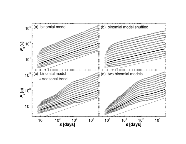
Figure 8: The fluctuation functions $F_{q}(s)$ obtained from the multifractal DFA4 for surrogate series generated by the extended multiplicative cascade model with parameters $a=0.50$ and $b=0.68$, that correspond to the values we obtained for the river Weser. The fluctuation function $F_{q}(s)$ for (a) the original $\phi_{i}$ series and (b) the shuffled series are plotted versus scale $s$ for the same values of $q$ as in Figs. 4 and 5. In (c) the $\phi_{i}$ have been multiplied by $0.1+\sin^{2}(\pi i/365)$ before the analysis to simulate a seasonal trend. In (d) modified values of the parameters $a$ and $b$ ($a=0.26$, $b=0.59$) have been used on scales $s\leq 256$ to simulate the apparent stronger multifractality on smaller scales observed for most rivers. For the figure, results from 10 surrogate series of length 140 years were averaged.

In order to see how well the extended multiplicative cascade model fits to the real data (for a given river), we generate the model data as follows: (i) we determine $a$ and $b$ for the given river (by best fit of Eq. (17)), (ii) we generate the simple multiplicative cascade model with the obtained $a$ and $b$ values, and (iii) we implement the proper long-term correlations as described above.

Figure 8(a) shows the DFA analysis of the model data with parameters $a$ and $b$ determined for the river Weser. By comparing with Fig. 4(a) we see that the extended model gives the correct scaling of the fluctuation functions $F_{q}(s)$ on time scales above the crossover. By comparing Fig. 8(b) with Fig. 4(c) we see that the shuffled model series becomes uncorrelated without multifractality similar to the shuffled data. Below the crossover, however, the model does not yield the observed $F_{q}(s)$ in the original data. In the following we show that in order to obtain the proper behaviour below the crossover, either seasonal trends that cannot be completely eliminated from the data or a different type of multifractality below the crossover, represented by different values of $a$ and $b$, have to be introduced.

To show the effect of seasonal trends, we have multiplied the elements $\phi_{i}$ of the extended cascade model by $0.1+\sin^{2}(\pi i/365)$, this way generating a seasonal trend of period 365 in the variance. Figure 8(c) shows the DFA4 result for the generalized fluctuation functions, which now better resembles the real data than Fig. 8(a). Finally, in Fig. 8(d) we show the effect of a different multifractality below the crossover, where different parameters $a$ and $b$ characterize this regime. The results also show better agreement with the real data. When comparing Figs. 8(a,c,d) with Figs. 4 and 5, it seems that the Danube, Amper and Wertach fit better to Fig. 8(d), i.e. suggesting different multifractality for short and large time scales, while the Weser, Susquehanna and Niger fit better to Fig. 8(c) where seasonal trends in the variance (and possibly in the skew) are responsible for the behaviour below the crossover.

4 Conclusion

In this study, we analyzed the scaling behaviour of daily runoff time series of 18 representative rivers in southern Germany and 23 international rivers using both Detrended Fluctuation Analysis and wavelet techniques. In all cases we found that the fluctuations exhibit self-affine scaling behaviour and long-term persistence on time scales ranging from weeks to decades. The fluctuation exponent $H$ varies from river to river in a wide range between 0.55 and 0.95, showing non-universal scaling behaviour.

We also studied the multifractal properties of the runoff time series using a multifractal generalization of the DFA method that was crosschecked with the WTMM technique. We found that the multifractal spectra of all 41 records can be described by a ’universal’ function $\tau(q)=-\ln(a^{q}+b^{q})/\ln 2$, which can be obtained from a generalization of the multiplicative cascade model and has solely two parameters $a$ and $b$ or, equivalently, the fluctuation exponent $H={1\over 2}-\ln(a^{2}+b^{2})/\ln 4$ and the width $\Delta\alpha=\ln{a\over b}/\ln 2$ of the singularity spectrum. Since our function for $\tau(q)$ applies also for negative $q$ values, we could derive the singularity spectra $f(\alpha)$ from the fits. We have calculated and listed the values of $H$, $a$, $b$, and $\Delta\alpha$ for all records considered. There are no significant differences between their distributions for rivers in South Germany and for international rivers. We also found that there is no significant dependence of these parameters on the size of the basin area, but there is a slight decrease of the multifractal width $\Delta\alpha$ with increasing basin area. We suggest that the values of $H$ and $\Delta\alpha$ can be regarded as ’fingerprints’ for each station or river, which can serve as an efficient non-trivial test bed for the state-of-the-art precipitation-runoff models.

Apart from the practical use of Eq. (17) with the parameters $a$ and $b$ that was derived by extending the multiplicative cascade model and that can serve as finger prints for the river flows, we presently are lacking a physical model for this behaviour. It will be interesting to see, if physically based models, e.g. the random tree-structure model presented in Gupta et al. (1996), can be related to the multiplicative cascade model presented here. If so, this would give a physical explanation for how the multiplicative cascade model is able to simulate river flows.

We have also investigated the origin of the multifractal scaling behaviour by comparison with the corresponding shuffled data. We found that the multifractality is removed by shuffling that destroys the time correlations in the series while the distribution of the runoff values is not altered. After shuffling, we obtain $h(q)\approx 1/2$ for all values of $q$, indicating monofractal behaviour. Hence, our results suggest that the multifractality is not due to the existence of a broad, asymmetric (singular) probability density distribution (Anderson and Meerschaert, 2002), but due to a specific dynamical arrangement of the values in the time series, i.e. a self-similar ’clustering’ of time patterns of values on different time scales. We believe that our results will be useful also to improve the understanding of extreme values (singularities) in the presence of multifractal long-term correlations and trends.

Finally, for an optimal water management in a given basin, it is essential to know, whether an observed long-term fluctuation in discharge data is due to systematic variations (trends) or the results of long-term correlation. Our approach is also a step forward in this directions.

Acknowledgments: We would like to thank Daniel Schertzer and Diego Rybski for valuable discussions. This work was supported by the BMBF, the DAAD, and the DFG. We also would like to thank the Water Management Authorities of Bavaria and Baden-Württemberg (Germany), and the Global Runoff Center (GRDC) in Koblenz (Germany) for providing the observational data.

References

- Anderson and Meerschaert (2002) Anderson, P.L., Meerschaert, M.M., 1998. Modelling river flows with heavy tails. Water Resources Research, 34(9), 2271-2280.
- Arneodo et al. (2002) Arneodo, A., Audit, B., Decoster, N., Muzy, J.-F., Vaillant, C., 2002. Wavelet based multifractal formalism: Applications to DNA sequences, satellite images of the cloud structure, and stock market data. In: Bunde et al. (2002), pp. 27-102.
- Barabasi and Vicsek (1991) Barabasi, A., Vicsek, T., 1991. Multifractality of self-affine fractals. Phys. Rev. A, 44, 2730-2733.
- Bunde et al. (2000) Bunde, A., Havlin, S., Kantelhardt, J.W., Penzel, T., Peter, J.-H., Voigt, K., 2000. Correlated and uncorrelated regions in heart-rate fluctuations during sleep. Phys. Rev. Lett., 85(17), 3736-3739.
- Bunde et al. (2002) Bunde, A., Kropp, J., Schellnhuber, H.-J. (eds.), 2002. The science of disaster: Climate disruptions, market crashes, and heart attacks. Springer, Berlin.
- Davis et al. (1996) Davis, A., Marshak, A., Wiscombe, W., Cahalan, R., 1996. Multifractal characterization of intermittency in nonstationary geophysical signals and fields. In: Current topics in nonstationary analysis, edited by Trevino, G., Harding, J., Douglas, B., Andreas, E., World Scientific, Singapore, pp. 97-158.
- Eichner et al. (2003) Eichner, J. F., Koscielny-Bunde, E., Bunde, A., Havlin, S., Schellnhuber, H.-J., 2003. Power-law persistence and trends in the atmosphere: A detailed study of long temperature records. Phys. Rev. E, 68, 046133.
- Feder (1988) Feder, J., 1988. Fractals. Plenum Press, New York.
- Frisch and Parisi (1985) Frisch, U., Parisi, G., 1985. Fully developed turbulence and intermittency, in: Turbulency and predictability in geophysical fluid dynamics. Edited by Ghil, M., Benzi, R., Parisi, G., North Holland, New York, pp. 84-92.
- Gupta et al. (1994) Gupta, V.K., Mesa, O.J., Dawdy, D.R., 1994. Multiscaling theory of flood peaks: Regional quantile analysis. Water Resources Research, 30(12), 3405-3421.
- Gupta and Dawdy (1995) Gupta, V.K., Dawdy, D.R., 1995. Physical Interpretations of regional variations in the scaling exponents of flood quantiles. In: Kalma, J.D., Scale issues in hydrological modelling, Wiley, Chichester, pp. 106-119.
- Gupta et al. (1996) Gupta V.K., Castro, S.L., Over, T.M., 1996. On scaling exponents of spatial peak flows from rainfall and river network geometry. J. Hydrol., 187(1-2), 81-104.
- Hurst (1951) Hurst, H.E., 1951. Long-term storage capacity of reservoirs. Transactions of the American Society of Civil Engineering, 116, 770-799.
- Hurst et al. (1965) Hurst, H.E., Black, R.P., Simaika, Y.M., 1965. Long-term storage: An experimental study. Constable & Co. Ltd., London.
- Kantelhardt et al. (2001) Kantelhardt, J.W., Koscielny-Bunde, E., Rego, H.H.A., Havlin, S., Bunde, A., 2001. Detecting long-range correlations with detrended fluctuation analysis. Physica A, 295, 441-454.
- Kantelhardt et al. (2002) Kantelhardt, J. W., Zschiegner, S.A., Koscielny-Bunde, E., Havlin, S., Bunde, A., Stanley, H.E., 2002. Multifractal detrended fluctuation analysis of nonstationary time series. Physica A, 316, 87-114.
- Kantelhardt et al. (2003) Kantelhardt, J. W., Rybski, D., Zschiegner, S.A., Braun, P., Koscielny-Bunde, E., Livina, V., Havlin, S., Bunde, A., 2003. Multifractality of river runoff and precipitation: Comparison of fluctuation analysis and wavelet methods. Physica A, 330, 240-245.
- Koscielny-Bunde et al. (1998) Koscielny-Bunde, E., Bunde, A., Havlin, S., Roman, H.E., Goldreich, Y., Schellnhuber, H.-J., 1998. Indication of a universal persistence law governing atmospheric variability. Phys. Rev. Lett., 81(3), 729-732.
- Lavallee et al. (1993) Lavallee, D., Lovejoy, S., Schertzer, D., 1993. Nonlinear variability and landscape topography: analysis and simulation. In: Fractals in Geography. PTR Prentic-Hall, edited by DeCola, L., Lam, N., pp. 158-192, 1993.
- Livina et al. (2003a) Livina, V. N., Ashkenazy, Y., Braun, P., Monetti, R., Bunde, A., Havlin, S., 2003a. Nonlinear volatility of river flux fluctuations. Phys. Rev. E, 67, 042101.
- Livina et al. (2003b) Livina, V., Ashkenazy, Y., Kizner, Z., Strygin, V., Bunde, A., Havlin, S., 2003b. A stochastic model of river discharge fluctuations, Physica A, 330, 283-290.
- Lovejoy and Schertzer (1991) Lovejoy, S., Schertzer, D., 1991. Nonlinear Variability in Geophysics: Scaling and Fractals. Kluver Academic Publ., Dortrecht, Netherlands.
- Mandelbrot and Wallis (1968) Mandelbrot, B. B., Wallis, J. R., 1968. Noah, Joseph, and operational hydrology. Water Resources Research, 4(5), 909.
- Mandelbrot and Wallis (1969) Mandelbrot, B. B., Wallis, J. R., 1969. Some long-run properties of geophysical records. Water Resources Research, 5(2), 321-340.
- Matsoukas et al. (2000) Matsoukas C., Islam, S., Rodriguez-Iturbe, I., 2000. Detrended fluctuation analysis of rainfall and streamflow time series. J. Geophys. Res. Atmosph., 105(D23), 29165-29172.
- Montanari et al. (2000) Montanari, A., Rosso, R., Taqqu, M. S., 2000. A seasonal fractional ARIMA model applied to the Nile River monthly flows at Aswan. Water Resources Research, 36(5), 1249-1259.
- Pandey et al. (1998) Pandey, G., Lovejoy, S., Schertzer, D., 1998. Multifractal analysis of daily river flows including extremes for basins of five to two million square kilometers, one day to 75 years. Journal of Hydrology, 208, 62-81.
- Peng et al. (1994) Peng, C.-K., Buldyrev, S. V., Havlin, S., Simons, M., Stanley, H. E., Goldberger, A. L., (1994). Mosaic organization of DNA nucleotides, Phys. Rev. E,49(2), 1685-1689.
- Peters et al. (2002) Peters, O., Hertlein, C., Christensen, K., 2002. A Complexity View of Rainfall. Phys. Rev. Lett., 88, 018701.
- Rodriguez-Iturbe and Rinaldo (1997) Rodriguez-Iturbe, I., Rinaldo, A., 1997. Fractal River Basins – Change and Self-Organization. Cambridge University Press, Cambridge.
- Schertzer and Lovejoy (1987) Schertzer, D., Lovejoy, S., 1987. Physical modelling and analysis of rain and clouds by anisotropic scaling multiplicative processes. J. Geophys. Res. Atmosph., 92, 9693.
- Sivapalan et al. (2002) Sivapalan, M., Jothityangkoon, C., Menabde, M., 2002. Linearity and nonlinearity of basin response as a function of scale: Discussion of alternative definitions. Water Resour. Res., 38, 1012.
- Talkner and Weber (2000) Talkner, P., Weber, R. O., 2000. Power spectrum and detrended fluctuation analysis: Application to daily temperatures. Phys. Rev. E, 62(1), 150-160.
- Taqqu et al. (1995) Taqqu, M. S., Teverovsky, V., Willinger, W., 1995. Estimators for long-range dependence: An empirical study. Fractals 3, 785-798.
- Tessier et al. (1996) Tessier, Y., Lovejoy, S., Hubert, P., Schertzer, D., Pecknold, S., 1996. Multifractal analysis and modelling of rainfall and river flows and scaling, causal transfer functions. J. Geophys. Res. Atmosph., 101(D21): 26427-26440.
- Turcotte and Greene (1993) Turcotte, D. L., Greene, L., 1993. A scale-invariant approach to flood-frequency analysis. Stoch. Hydrol. Hydraul., 7, 33-40.
- Weber and Talkner (2001) Weber, R. O., Talkner, P., 2001. Spectra and correlations of climate data from days to decades. J. Geophys. Res. Atmosph., 106(D17), 20131.