Diamagnetic Suppression of Component Magnetic Reconnection at the Magnetopause

Abstract

We present particle-in-cell simulations of collisionless magnetic reconnection in a system (like the magnetopause) with a large density asymmetry across the current layer. In the presence of an ambient component of the magnetic field perpendicular to the reconnection plane the gradient creates a diamagnetic drift that advects the X-line with the electron diamagnetic velocity. When the relative drift between the ions and electrons is of the order the Alfvén speed the large scale outflows from the X-line necessary for fast reconnection cannot develop and the reconnection is suppressed. We discuss how these effects vary with both the plasma $\beta$ and the shear angle of the reconnecting field and discuss observational evidence for diamagnetic stabilization at the magnetopause.

SWISDAK ET AL. DIAMAGNETIC SUPPRESSION OF RECONNECTION M. Swisdak, IREAP, University of Maryland, College Park, MD 20742-3511, USA, (swisdak@glue.umd.edu)

1 Introduction

Magnetic reconnection, the breaking and reforming of magnetic field lines with a concomitant transfer of energy from the field to the surrounding plasma, is thought to drive such phenomena as solar flares, magnetospheric substorms, and tokamak sawtooth crashes. Despite the suspected linkage, the resistive magnetohydrodynamic (MHD) model of reconnection due to Sweet [1958] and Parker [1957] (the favored theoretical model for many years), predicts reconnection rates in each of these systems that are typically orders of magnitude too low to be physically relevant. The discrepancy arises because the Sweet-Parker reconnection rate varies with the Spitzer resistivity which in turn depends on particle interactions that are rare in these collisionless plasmas.

Recent work suggests that terms important at small length scales but usually ordered away in resistive MHD, notably the Hall term in Ohm’s law, lead to reconnection rates that are consistent with the observations [Shay et al., 1999]. With the addition of this new physics the speed of the electron flows away from the reconnection site (the X-line) is no longer bounded by the ion Alfvén speed, instead scaling inversely with the width of the current layer formed by the reconnecting magnetic fields. As a result, the outward electron flux remains large even as the width, controlled by non-ideal effects, becomes small. Downstream from the reconnection site the super-Alfvénic electrons slow to rejoin the ions and expand outwards in a wide layer reminiscent of the Petschek [1964] model. This behavior has been confirmed by a variety of numerical simulations: two-fluid, hybrid (fluid electrons and particle ions), and full particle. In the GEM (Geospace Environment Modeling) reconnection challenge each of several independent codes modeling an identical (two-dimensional) system found features similar to those described above [Birn et al., 2001 and references therein]. Laboratory experiments in the relevant regimes are challenging, but recent results [Brown, 1999; Ji et al., 1999] support some aspects of this picture.

Although the GEM challenge established a possible mechanism for fast collisionless reconnection, it did so for a relatively simple geometry. Experimental evidence suggests that in nature reconnection is likely to be more complex. For instance, at the Earth’s dayside magnetopause the magnetosphere, a region of low density but strong magnetic field, abuts the magnetosheath and its high density but weaker magnetic field. Still, early single-point spacecraft measurements of the magnetopause [Paschmann et al., 1979; Sonnerup et al., 1981] detected field signatures and particle distribution functions suggesting the occurrence of reconnection. A more recent study using data from multiple spacecraft [Phan et al., 2000] found, at least in one case, the bidirectional jets that are a reconnection hallmark. Similar cross-field pressure gradients occur in laboratory fusion experiments where their associated diamagnetic drifts are thought to control the onset of reconnection during the sawtooth crash [Levinton et al., 1994].

The first theoretical explorations of asymmetric reconnection [Levy et al., 1964; Petschek and Thorne, 1967] were based on incompressible MHD and predict an outflow region comprising a combination of slow MHD shocks and slow and intermediate MHD waves. Two-dimensional computer simulations using compressible MHD [Hoshino and Nishida, 1983; Scholer, 1989], hybrid [Lin and Xie, 1997; Omidi et al., 1998; Krauss-Varban et al., 1999; Nakamura and Scholer, 2000] and particle [Okuda, 1993] codes have addressed these predictions. Common features include the preferential growth of the magnetic island (O-line) towards the magnetosheath and a pronounced density drop on the magnetospheric side of the boundary layer. Also, consistent with the picture of Levy et al. [1964], the current layer abutting the magnetosheath is generally stronger than that bordering the magnetosphere and takes the form of a series of discontinuities. There is disagreement, however, concerning the precise form of these discontinuities, possibly because the nonlocality associated with the motion of collisionless particles parallel to the shock front makes the two-dimensional (2-D) simulations more complicated than the 1-D models. Simulations have also been performed with an initial out-of-plane component of the magnetic field (nonzero $B_{y}$ in GSM coordinates) [Hoshino and Nishida, 1983; Krauss-Varban et al., 1999; Nakamura and Scholer, 2000]. This guide field tends to slow, but not completely suppress, reconnection and alter the structure of the shock transitions.

In our investigations we begin with a simple magnetopause equilibrium model with an ambient pressure difference and perform two-dimensional fully kinetic numerical simulations. We reproduce the qualitative features seen in previous work but also find that diamagnetic drifts produced by the pressure gradient advect the X-line. When the diamagnetic velocity, $\mathbf{v}_{*}=-(c/qnB^{2})\bm{\nabla}p\bm{\times}\mathbf{B}$ ($c$ is the speed of light; $q$, $n$, and $p$ are the species charge, density, and pressure; $\mathbf{B}$ is the magnetic field), is comparable to the Alfvén speed, reconnection is completely suppressed. These diamagnetic effects have not been previously reported in the context of magnetopause reconnection. They are ordered out of the MHD model [Hoshino and Nishida, 1983] and were not seen in the hybrid simulations, perhaps because the spatially localized resistivity used to trigger fast reconnection effectively prohibits X-line advection. In spite of this, diamagnetic effects can be significant at the magnetopause. Taking $n\sim 10\text{ cm}^{-3}$, $B\sim 10^{-4}\text{ G}$, $k_{B}T\sim 100\text{ eV}$, and gradients of order an inverse ion inertial length, one finds $v_{*}/v_{A}\sim 1$. In the fusion context, previous analytic work has suggested that diamagnetic drifts can stabilize the tearing mode and lower the rate of reconnection [Biskamp, 1981; Rogers and Zakharov, 1995]. But since this work considered a reduced MHD model (equivalent to the limit of a large guide field) its applicability to magnetospheric applications has not been established.

Unlike the configuration in the magnetotail, the magnetic field on opposite sides of the magnetopause is usually not equal in magnitude and anti-parallel. Reconnection in such a system does not occur at a unique spatial location, even in a model with a 1-D equilibrium, since components of the magnetic field reverse direction at any location across the current layer. Because of the possibility that reconnection can occur at multiple spatial locations, it has been suggested that the magnetopause magnetic field is stochastic [Galeev et al., 1986; Lee et al., 1993]. The exploration of reconnection in a 2-D model must then be carried out with care since stability at a particular surface does not necessarily imply stability at all surfaces. In exploring the impact of diamagnetic drifts on reconnection we therefore must address both stability at a single plane and explore which plane is expected to dominate the dynamics of a full 3-D system. We suggest on the basis of analytic arguments and simulations that the strongest reconnection occurs at the surface where the reversed field components have equal magnitudes.

In section 2 of the paper we present our computational scheme and initial conditions. Section 3 is an overview of reconnection at the magnetopause, both without and with a diamagnetic drift. Section 4 discusses how varying the strength of the out-of-plane field changes the diamagnetic effects while section 5 addresses the question of determining the dominant reconnection plane. Finally, in section 6 we summarize our results and discuss their implications for understanding magnetic reconnection at the magnetopause.

2 Computational Methods

Although diamagnetic drifts are present in two-fluid and hybrid models, a complete calculation in the collisionless limit requires a careful, and assumption-filled, treatment of the full pressure tensor. To avoid this difficulty, we sacrifice the benefits of a fluid simulation for a more computationally demanding, but mathematically straightforward, full particle description.

2.1 The Code

The simulations are done with p3d, a massively parallel kinetic code that can evolve up to $\sim\negmedspace 10^{9}$ particles on current Cray T3E and IBM SP systems [Zeiler et al., 2002]. The Lorentz equation of motion for each particle is evolved by a Boris algorithm ($\mathbf{E}$ accelerates for half a timestep, followed by a rotation of $\mathbf{v}$ by $\mathbf{B}$, and then the other half-step acceleration by $\mathbf{E}$). The electromagnetic fields are advanced in time with an explicit trapezoidal-leapfrog method using second-order spatial derivatives. Poisson’s equation constrains the system; if $\bm{\nabla\cdot}\mathbf{E}\neq 4\pi\rho$, a multigrid algorithm recursively corrects the electric field. Although the code permits other choices, we work with fully periodic boundary conditions.

The code is written in normalized units: lengths to the ion inertial length $c/\omega_{pi}=d_{i}$, times to the inverse ion cyclotron frequency $\Omega_{ci}^{-1}$, velocities to the Alfvén speed $v_{A}$, masses to the ion mass $m_{i}$, and temperatures to $m_{i}v_{A}^{2}$. Unless otherwise noted, the asymptotic reconnecting field is assumed to have a magnitude of $1$ on both sides of the magnetopause (the reason for this choice will be made clear in section 5) and the asymptotic density in the magnetosheath is taken to be $1$.

To conserve computational resources, yet assure a sufficient separation of spatial and temporal scales, we take the electron mass to be $0.005=1/200$ and the speed of light to be $20$. Our simulations are performed in a box of $1024\times 1024$ gridpoints that is $25.6$ on a side, corresponding to a grid scale of $0.025$ and so $\approx\negmedspace 3$ gridpoints per electron inertial length. A typical timestep is $1.5\times 10^{-3}$.

2.2 Initial Conditions

Reconnection occurs in the $x-y$ plane in our coordinate system. For reference, this is equivalent to the $z-x$ plane in GSM coordinates. The initial equilibrium is constructed from two (modified) Harris current sheets centered at $L_{y}/4$ and $3L_{y}/4$, where $L_{y}$ is the box size in the $y$ direction; to allow periodicity the current is parallel to $\mathbf{\hat{z}}$ in one sheet and anti-parallel in the other. The current sheets produce a magnetic field $B_{x}=\tanh[(y-L_{y}/4)/w_{0}]-\tanh[(y-3L_{y}/4)/w_{0}]-1$, where $w_{0}=0.5$. The density profile is similar, $n=n_{0}(\tanh[(y-L_{y}/4)/w_{0}]-\tanh[(y-3L_{y}/4)/w_{0}])+n_{\text{min}}$, where, unless otherwise specified, $n_{0}=0.45$ and $n_{\text{min}}=0.1$. This profile gives an asymptotic density of $n=1$ in the magnetosheath and $0.1$ in the magnetosphere. The initial ion and electron temperatures are $T_{i}=2$ and $T_{e}=1$, implying thermal speeds of $\approx 1.4\text{ and }14$, respectively. The guide (out-of-plane) field $B_{z}$ is assigned a specific asymptotic value $B_{z0}$ on the magnetosheath side and is calculated elsewhere by assuming pressure balance. Note that at the reversal surface, where $B_{x}=0$, pressure balance implies that $\partial_{y}n(T_{i}+T_{e})\propto B_{z}\partial_{y}B_{z}$, and hence a density gradient must be accompanied by a gradient in $B_{z}$. At $t=0$ a 5% perturbation in the magnetic flux function places the X- and O-line in each sheet.

Unlike a conventional Harris sheet, this initial state is not a kinetic (Vlasov) equilibrium. Although it has been shown [Quest and Coroniti, 1981] that the presence of a guide field reduces the growth rate of the tearing mode instability in the linear regime, our initial perturbation is large enough that the system begins to reconnect nonlinearly before any other perturbations become important. We must also emphasize that our system characterizes the magnetopause only in a rough approximation. In particular, magnetospheric plasma is typically not isothermal, but instead has temperature gradients comparable in magnitude, but anti-parallel, to those of the plasma density. If this effect is included the overall pressure gradient, as well as the diamagnetic effects we discuss here, will be smaller.

3 Simulation Overview

In the simplest description of fast collisionless reconnection three length scales are relevant: the system size and the ion and electron inertial lengths. (Depending on the strength of the initial out-of-plane field, the ion Larmor radius can also enter as a parameter [Kleva and Drake, 1995].) The dynamic couplings between these scales, which must exist for fast reconnection to occur, are discussed in detail by Biskamp et al. [1997] and Shay et al. [1998]. At large scales both species are frozen into the magnetic field and flow towards the X-line with a velocity $v_{in}$ that is some fraction of the upstream Alfvén speed. Roughly $c/\omega_{pi}$ away from the current sheet the inertia term in the ion equation of motion becomes important and the ions, but not the electrons, decouple from the field. Deflected outwards, the ions flow Alfvénically away from the X-line while the electrons travel further inward until they too decouple and travel outward at velocities near the electron Alfvén speed. Downstream, the electrons slow to join the ionic outflow and reform an MHD fluid. In what follows we show that diamagnetic drifts can disrupt this structure by strongly altering the MHD outflows, thereby inhibiting the coupling of the ions to the X-line and halting the formation of a large-scale reconnection geometry.

3.1 Anti-parallel Reconnection

To document certain features and establish contact with previous work, Figure 1 shows the X-line structure from a magnetopause simulation similar to those described by Krauss-Varban et al. [1999] and Nakamura and Scholer [2000]. The upper section of each panel ($y/d_{i}>3.2$) contains low density plasma and a large magnetic field like the magnetosphere, while the lower section has a high density plasma and a weak field like the magnetosheath. There are a few differences between the initial conditions for this simulation and the case with a guide field discussed in section 2.2 (and used in the rest of this paper). The reversed field is given by a shifted hyperbolic tangent such that the magnitudes of the asymptotic fields are unequal, $B_{x}^{sp}=1.5$ and $B_{x}^{sh}=0.5$, where magnetosphere and magnetosheath quantities are denoted with the superscripts “sp” and “sh”, respectively. The guide field $B_{z}$ is zero. Pressure balance then fixes the density profile as a gradient from $1$ to $2/3$ across the current layer with a relative maxima where $B_{x}=0$.

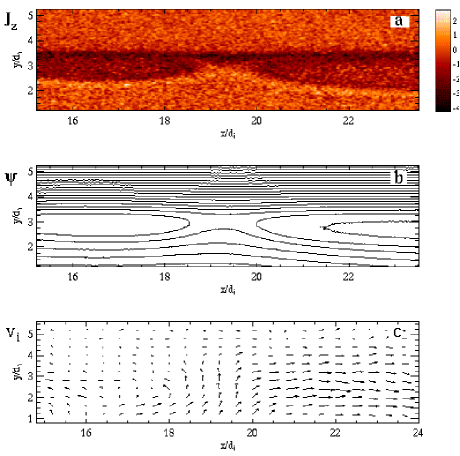
Figure 1: Reconnection in a magnetopause-like configuration with no guide field. In each panel $t=13.5\Omega_{ci}^{-1}$. (a) The out-of-plane current density $J_{z}$, (b) the in-plane field lines, and (c) the ion velocity vectors, averaged over a scale of $\sim d_{i}$. Note the flows associated with the X-line. The longest vector corresponds to a velocity of $\sim 0.15v_{A}$.

The general features of Figure 1 are consistent with earlier calculations. One consequence of the asymmetry in field strengths across the magnetopause is the evident tendency for the magnetic island to grow preferentially in the direction of the magnetosheath. Since equal amounts of flux must reconnect from either side in a given time, $B^{sp}v_{in}^{sp}=B^{sh}v_{in}^{sh}$, and so $v_{in}^{sh}=(B^{sp}/B^{sh})v_{in}^{sp}\gg v_{in}^{sp}$. The larger inflow on the magnetosheath side of the reversal surface is evident in the ion velocity vectors shown in Figure 1c. With the stronger inflow, the (frozen-in) magnetosheath field is more strongly advected toward the X-line than its magnetospheric counterpart, leading to the wider opening angle (i.e., the bulge) on the magnetosheath side of the current layer. In earlier MHD simulations it was shown that the asymmetry of the island did not appear when the amplitudes of the reversed field on either side of the magnetopause are equal [Scholer, 1989].

Because of the simulation’s relatively small size clearly separated MHD and kinetic discontinuities do not exist, making comparisons with previous work difficult. Nevertheless, in cuts of the reconnection outflow (see Figure 2), the self-generated, out-of-plane magnetic field is evident and the positive (negative) value of $B_{z}$ on the magnetosheath (magnetosphere) side of the current layer is consistent with earlier predictions. The perturbation, however, is much stronger on the magnetosheath side; the anti-symmetry of $B_{z}$ seen in systems with a symmetric pressure does not extend to reconnection at the magnetopause.

Figure 2: Cuts at $x=20d_{i}$ of the outflow region of Figure 1. Each plot has been averaged over $0.25d_{i}$ in the horizontal direction to reduce the noise. (a)-(c) The reconnecting field, the out-of-plane field, and the density, respectively.

The sharp density drop at the magnetosphere edge of the current layer ($y\approx 3.4d_{i}$) is a consequence of the different inflow speeds on the two sides of the layer and the plasma mixing across the island. Since the magnetospheric field is much stronger, and therefore the inflow velocity from this side of the current layer is weak, only a small amount of magnetospheric plasma crosses the separatrices. The result is an outflow region almost completely comprising magnetosheath plasma. This effect was evident in earlier hybrid simulations [Krauss-Varban et al. 1999; Nakamura and Scholer, 2000] and has also been seen in satellite crossings of the magnetopause [Eastman et al., 1996].

3.2 Component Reconnection and Diamagnetic Propagation

In the presence of a magnetic field any nonparallel pressure gradient produces a diamagnetic drift,

$$\mathbf{v}_{*j}=-c\frac{\bm{\nabla}p_{j}\bm{\times}\mathbf{B}}{q_{j}nB^{2}}\text{,}$$ (1)

where $p_{j}=nT_{j}$ is the thermal pressure and $q_{j}$ is the charge of species $j$. Due to the charge dependence, ions and electrons drift in opposite directions. To have diamagnetic flows parallel to the current layer in our geometry the guide field $B_{z}$ and the gradient of the pressure must be nonzero where $B_{x}=0$.

Even though diamagnetic drifts do not correspond to actual particle motions they nevertheless advect the magnetic field [Coppi, 1965; Scott and Hassam, 1987]. In two dimensions the magnetic field can be written as $\mathbf{B}=\mathbf{\hat{z}}\bm{\times\nabla}\psi(x,y)+B_{z}(x,y)\mathbf{\hat{z}}$ where $\psi$ is the magnetic flux function. Taking the cross product of Faraday’s law with $\mathbf{\hat{z}}$ yields $\partial_{t}\bm{\nabla}\psi-c\bm{\nabla}E_{z}=0$, or $E_{z}=\partial_{t}\psi/c$. Next, dotting the electron fluid equation with $\mathbf{\hat{z}}$ gives

$$E_{z}=-\frac{1}{c}\mathbf{\hat{z}}\cdot(\mathbf{v_{e}}\bm{\times}\mathbf{B})-\frac{m_{e}}{e}\frac{dv_{ez}}{dt}\text{.}$$ (2)

The last term represents the inertial effects of electrons and breaks the frozen-in condition. Since it is usually small we ignore it and substitute for $\mathbf{B}$ to get $E_{z}=-\mathbf{v_{e}}\bm{\cdot\nabla}\psi/c$ and a convection equation for the flux [Coppi, 1965],

$$\partial_{t}\psi+\mathbf{v_{e}}\bm{\cdot\nabla}\psi=0\text{.}$$ (3)

Hence, the electron fluid velocity, which includes a diamagnetic component given by (1), advects magnetic structures.

Strictly speaking, equations (1) and (3) are fluid results and need not describe the dynamics at the X-line of our simulations where small-scale structures leave the fluid approximation on unsure ground. However, as can be seen in Figure 3, they are still good descriptions of the system. The out-of-plane current density essentially maps the magnetic field lines (see Figure 1b) so the island (centered at $x/d_{i}\sim 5$) grows robustly during the time shown. Simultaneously, the X-line propagates to the left, the direction of the electron diamagnetic drift. The locations of the X-line in the three panels of Figure 3 are $x/d_{i}=19.2$, $14.8$ and $10$, respectively, corresponding to a drift speed of $0.61v_{A}$ and consistent with the value calculated from the initial parameters of $v_{*e}=0.56$. As flux reconnects the magnetic island widens, decreasing the pressure gradient across its center, slowing its drift, and allowing the X-line to overtake it. This stabilizes the island’s growth because the plasma outflow from the X-line towards the near end of the island must slow due to the increase in magnetic pressure. The actual collision of the X-line with the island, which occurs later in time, may be unphysical since in any real system the initial separation of the X- and O-lines will be much greater than the $12.8d_{i}$ of the present model. Thus, the effects of the collision will not be discussed further.

A surprise is that the diamagnetic propagation evident in Figure 3 has not been seen in previous hybrid simulations of the magnetopause [Krauss-Varban et al., 1999; Nakamura and Scholer, 2000] even though these models should include the relevant electron diamagnetic drifts. In some cases the simulation parameters may be such as to minimize diamagnetic effects (e.g. a lower magnetospheric temperature). Diamagnetic drifts may also be absent if the simulations were performed with an initially uniform out-of-plane field. According to the force balance condition, the local pressure gradient (and hence the drift) must then be zero at the reversal surface, although whether it would remain zero as the system evolves is unclear. In section 5 we discuss further why a uniform guide field may not be representative of reconnection at the magnetopause. A final possibility occurs for simulations using a fixed, spatially-localized resistivity to break the frozen-in condition at the X-line. How such a resistivity model would affect an X-line that is trying to propagate is unclear, but it is nevertheless evident from our results that such models may be inappropriate for simulating guide field reconnection at the magnetopause when diamagnetic drifts are large.

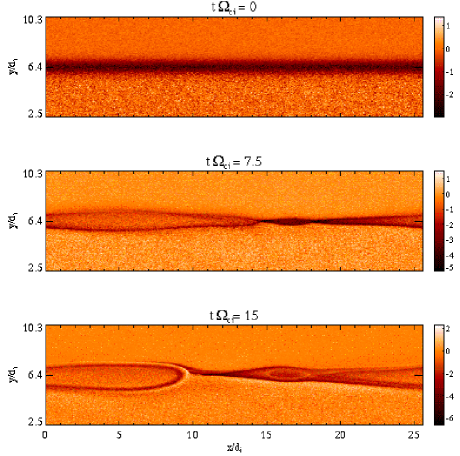
Figure 3: The out-of-plane current density at three times for a magnetopause geometry similar to Figure 1, but including an out-of-plane guide field and therefore an in-plane diamagnetic drift. The initial conditions are those described in section 2.2 with an asymptotic guide field of $3.0$ in the magnetosheath and $3.8$ in the magnetosphere. The density drops from $1$ to $0.1$ across the current layer.

Figure 4a shows the current density for the simulation of Figure 3. Unlike the example shown in Figure 1, the magnetic island does not bulge into the magnetosphere side of the current layer. This is because the reconnecting magnetic field $B_{x}$ is anti-symmetric across the current layer and thus, as discussed earlier, both sides contribute equal amounts of magnetic flux to the reconnection. Clearly evident in Figure 4a, as well as the last two panels of Figure 3, is the left-right asymmetry of the opening angle of the magnetic field lines near the X-line. This is caused by the interplay of the X-line’s diamagnetic drift, controlled by just the electrons, and the reconnection outflow, which must also involve the ions.

Consider the relative motion of the X-line and the ions. Downstream from the reconnection site the $\mathbf{J}\bm{\times}\mathbf{B}$ force accelerates frozen-in ions up to the Alfvén speed, $\pm v_{Ax}$. To this must be added the relative velocity between the diamagnetic drift of the ions and the X-line, $v_{*}=|v_{*i}|+|v_{*e}|$, with the result being a right-left asymmetry in the outflow velocities, $\pm v_{Ax}+v_{*}$. Since, from continuity, the opening angle of the magnetic field downstream from the X-line is roughly $v_{in}/v_{out}$ — and $v_{in}$ is roughly constant due to the symmetric reconnecting field — we expect the rightward opening angle to be much smaller than its counterpart, consistent with Figure 4b.

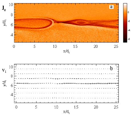
Figure 4: Structure of (a) the out-of-plane current density $J_{z}$ and (b) ion flow vectors at $t=16.0\Omega_{ci}^{-1}$ for the simulation shown in Figure 3. The large flows at the current layer are the ion diamagnetic drifts. The longest vector corresponds to a velocity of $\sim 1.2v_{A}$

By a similar argument, normal ion outflow from an X-line only develops when $v_{Ax}>v_{*}$. For the simulations presented in Figures 3 and 4 the electron and ion diamagnetic drifts at the reversal surface are $-0.56$ and $1.12$, respectively, compared with $v_{Ax}=1.35$ (based on a density of $0.55$, corresponding to a mixture of the magnetopause and magnetosheath plasma). Thus, for the parameters of this simulation, the reconnection should be marginally unable to reverse the ion flow to the left of the X-line. The ion flow vectors are shown in Figure 4b at the same time as the current density shown in Figure 4a. The strong ion flow on the right side of the X-line results from the combination of the ion diamagnetic velocity with the direct acceleration by the reconnected magnetic field. The reconnection generated forces almost reverse the diamagnetic flow just to the left of the X-line.

We again emphasize that it is the relative drift of the ions and electrons, i.e. $v_{*}=|v_{*i}|+|v_{*e}|$, that must be smaller than the in-plane Alfvén speed for normal reconnection to proceed. Reconnection was suppressed in a nearly indistinguishable fashion in a series of simulations with the same total temperature $T_{e}+T_{i}$ (and therefore identical $v_{*}$) but differing values of $T_{e}$ and $T_{i}$ ($T_{i}=1/2,T_{e}=5/2$ and $T_{i}=5/2,T_{e}=1/2$). Since $T_{i}\gg T_{e}$ at the magnetopause, stabilization can still occur even if the drift of the X-line, which is due only to $v_{*e}$, is negligible.

The cuts in Figure 5 show that for this simulation the reconnection field $B_{x}$ is symmetric across the layer while the pressure drop across the magnetopause is supported by the jump in the guide field $B_{z}$. In contrast to the density profile in the case with no guide field, the density drop across the layer is nearly centered on the magnetic island. Large drops occur on either edge of the current layer with a weak plateau in the middle of the island. The inflow velocity into the island from either side of the current layer is now roughly equal because of the near anti-symmetry of $B_{x}$. The plasma in the core of the island is therefore a nearly equal mix of magnetosphere and magnetosheath plasma and is not dominated by the magnetosheath, in contrast to the case shown in section 3.1.

Figure 5: Cuts at $x=13.8d_{i}$ of the outflow region of Figure 4. Each plot has been averaged over $0.1d_{i}$ in the horizontal direction to reduce the noise. (a)-(c) The reconnecting field, out-of-plane field and density, respectively.

4 Suppression of Component Reconnection

We have shown for a single case that, consistent with equation (3), X-lines convect with the diamagnetic velocity of the electrons in the reversal region and suggested a criterion for the suppression of reconnection from diamagnetic drifts, $v_{*}>v_{Ax}$. We now more fully explore this stabilization criterion by varying the strength of the out-of-plane field to vary the ratio of $v_{*}$ to $v_{Ax}$. For our magnetopause model the diamagnetic velocity at the surface where $B_{x}=0$ can be written as

$$v_{*j}=\frac{cT_{j}}{q_{j}L_{pj}B_{z}},$$ (4)

where the pressure scale length is given by $L_{p}^{-1}=|\partial_{y}p|/p$. Varying the amplitude of the out-of-plane field $B_{z}$ while keeping all the other parameter fixed alters $v_{*j}$ but keeps $v_{Ax}$ constant. As can be seen in Figure 6a, a large guide field implies a small $v_{*}$. Despite the occasional glitches (discontinuities in the motion arise when a new X-line triggered by random perturbations begins to dominate), the drift velocity is remarkably constant.

The bottom panel of Figure 6 shows the initial electron diamagnetic velocity at the reversal surface versus the drift speed of the X-line measured in the simulation. Although the agreement for sub-Alfvénic velocities is quite good, as $v_{*e}$ approaches $v_{Ax}$ another effect becomes important. Rather than move the ions at super-Alfvénic velocities the system develops an electric field $E_{y}$ transverse to the current layer that, combined with the guide field $B_{z}$, generates an $\mathbf{E}\bm{\times}\mathbf{B}$ drift opposing the ion motion and adding to the electron velocity. There is no change in the net current but the electrons, and hence the X-line, move faster than just the diamagnetic velocity would suggest.

Figure 6: The top panel shows the position of the X-line versus time for several runs differing only in the strength of the guide field $B_{z}$. The solid line is for the run of section 3.1 and experiences no diamagnetic motion. The dotted, dashed, and dash-dotted lines correspond to $B_{z0}=3,1.5,$ and $0.5$, respectively. The bottom panel is a comparison of the measured X-line velocities and the electron diamagnetic velocity at the reversal surface. The straight line has a slope of one and is plotted to guide the eye. In both panels the X-point location corresponds to a saddle point in $\psi$.

Since diamagnetic flows of sufficient strength disrupt the large-scale flows characteristic of reconnection, increases in $v_{*}$ should correlate with decreases in the amount of reconnected flux. Figure 7 depicts the extent to which a diamagnetic drift can alter the reconnection rate of a system. The reconnected flux is plotted versus time for four different simulations: one with no diamagnetic drift, as in Figure 1, and three with varying asymptotic guide fields, $B_{z0}=1.5,1.0,$ and $0$. For the latter cases the associated drift speeds (diamagnetic plus $\mathbf{E}\bm{\times}\mathbf{B}$) at the reversal surface are $v_{*}=0.8,1.1$ and $1.5$, respectively. Reconnection is almost completely suppressed for the largest drifts. The plateau in reconnected flux seen in each of the bottom three curves is an artifact (discussed earlier) of our system’s periodic boundary conditions that allow the X-line to impinge on the more slowly propagating magnetic islands.

For large guide fields the diamagnetic drift speed approaches zero and the stabilization is minimized. The converse limit is more subtle since pressure balance imposes restrictions on the system’s configuration. If the profiles of the density and the reconnecting field are specified then there is a minimal possible value of the guide field in the current layer; $B_{z}$ cannot be taken to be zero and the drift cannot grow without bound. Hence although (for example) the GEM challenge simulations had zero guide field they did not have a large diamagnetic drift. Rather, $B_{z}\rightarrow 0$ and $L_{p}\rightarrow\infty$, keeping $v_{*}=0$.

Figure 7: Reconnected flux versus time for four simulations. The reconnection rate is the slope of each curve. The solid line is a reference run with no diamagnetic drift. The dotted, dashed, and dash-dotted lines are from simulations with differing values of $B_{z0}$ ($1.5,1.0$ and $0$, respectively) and therefore $v_{*}$.

To confirm the hypothesis that the reconnection process cannot reverse the ion diamagnetic drift and drive outward flows from the X-line for large values of the diamagnetic velocity, we show $J_{z}$ and the ion velocities from a simulation with an asymptotic out-of-plane field $B_{z}=0.5$ in Figure 8. In this case the island of reconnected flux remains small even at late time because of the weak growth shown in Figure 7. The flows are actually smaller than the peak of the expected diamagnetic velocity because of the development of the electric field $E_{y}$ across the layer. A slight reduction of the ion flow speed to the left of the X-line indicates that the reconnected field lines exert a small leftward directed force on the ions in this region, but the result is only a small perturbation of the ion flow pattern. Thus, the X-line is unable to couple effectively to the ions, strong reconnection does not develop, and the island amplitude saturates.

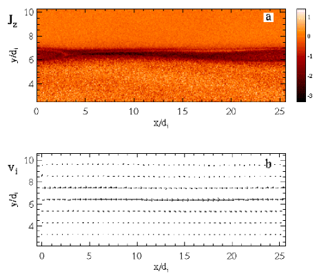
Figure 8: (a) The out-of-plane current density $J_{z}$ and (b) ion flow vectors at $t=13.0\Omega_{ci}^{-1}$ from a simulation with an asymptotic $B_{z}=0.5$ and a strong diamagnetic drift. The large flows to the right at the current layer are the result of the ion diamagnetic drift. The longest vector corresponds to a velocity of $\sim 0.95v_{A}$

.

5 Dependence on the Reconnection Plane

Although two-dimensional simulations are computationally cheaper than their three-dimensional counterparts, this simplicity comes with drawbacks. Perhaps the most important when considering diamagnetic drifts is that the orientation of the X-line with respect to the magnetic field configuration is externally imposed, rather than being free to develop. Different simulation planes have different reconnecting and out-of-plane fields and hence varying amounts of diamagnetic stabilization. In this section we explore this effect, albeit only by considering rotations around the $\mathbf{\hat{y}}$-axis to avoid introducing stabilizing $B_{y}$ components into the system. We will assume that the favored plane (i.e., the one the system would choose if allowed to evolve in three dimensions) is the one where the reconnection rate is maximal, but note that the results are not a replacement for more ambitious 3-D simulations. We further assume that the diamagnetic effects are playing the dominant role in determining the plane where reconnection is most robust. Thus, we are considering systems in which $v_{*}\sim v_{Ax}$.

Three-dimensional particle simulations have already addressed this issue for the basic case of a system with no guide field and no pressure drop across the current layer [Hesse et al., 2001; Pritchett, 2001]. Random perturbations were used as seeds to avoid imposing a plane a priori. Although X-lines were free to develop with any orientation, they preferentially formed parallel to the current layer, consistent with our assumption of treating only rotations about $\mathbf{\hat{y}}$. Moreover they remained quasi-two-dimensional even at late times. However, the simplicity of $\mathbf{B}$ makes this case degenerate since the reversal surface (the place where $B_{x}=0$) must be at the center of the current layer for any rotation about $\mathbf{\hat{y}}$. This restriction does not exist in more complicated configurations.

Figure 9: Schematic of the asymptotic magnetic fields in the magnetosphere, $B^{sp}$, and magnetosheath, $B^{sh}$. The reconnecting and out-of-plane components of the magnetic field depend on the orientation of the reconnection plane: $x-z$ versus $x^{\prime}-z^{\prime}$.

The basic geometry of magnetic fields at the magnetopause is shown in Figure 9. In order to agree with our simulation coordinates, the magnetospheric field $\mathbf{B}^{sp}$ is taken to be in the positive $x$ direction while the magnetosheath field $\mathbf{B}^{sh}$ is inclined at an angle $\theta$ with respect to the negative $x$ axis. Thus, the rotation angle across the magnetopause is $\pi-\theta$. The $\mathbf{\hat{y}}$ direction is perpendicular to the surface of the magnetopause. For a two-dimensional simulation in the $x-y$ plane the reconnecting components of the magnetic field will be parallel to $\mathbf{\hat{x}}$,

$$B^{sp}_{x}=B^{sp}$$ (5)

$$B^{sh}_{x}=-B^{sh}\cos\theta\text{,}$$ (6)

and the guide field to $\mathbf{\hat{z}}$,

$$B^{sp}_{z}=0$$ (7)

$$B^{sh}_{z}=B^{sh}\sin\theta\text{.}$$ (8)

The primed axes in Figure 9 are rotated clockwise by an angle $\alpha$ with respect to the unprimed system and represent another possible reconnection plane. In a simulation carried out in the $x^{\prime}-y^{\prime}$ plane the reconnecting components of the magnetic field will be

$$B^{sp}_{x^{\prime}}=B^{sp}\cos\alpha$$ (9)

$$B^{sh}_{x^{\prime}}=-B^{sh}\cos(\theta+\alpha)\text{,}$$ (10)

while the guide field components are

$$B^{sp}_{z^{\prime}}=-B^{sp}\sin\alpha$$ (11)

$$B^{sh}_{z^{\prime}}=B^{sh}\sin(\theta+\alpha)\text{.}$$ (12)

As shown in section 4, stabilization via a diamagnetic drift is inversely proportional to the value of the guide field $B_{z}$ in the center of the current layer. Thus, the expectation is that the plane with the maximum value of the guide field at the surface where reconnection takes place will dominate. Unfortunately, the asymptotic fields determine neither the location of the reversal surface nor the value of the guide field there. Furthermore, the actual guide field at the reversal surface may vary as reconnection proceeds. To simplify matters, we adopt the crude hypothesis that the guide field at the reversal surface $B_{g}$ is the mean of the asymptotic guide fields, which is $[B^{sh}\sin(\theta+\alpha)-B^{sp}\sin\alpha]/2$ in the rotated system. With this ansatz the optimal plane for reconnection is that where $B_{g}$ is maximized with respect to the angle $\alpha$, from which we derive the condition

$$B^{sp}\cos\alpha=B^{sh}\cos(\theta+\alpha)\text{.}$$ (13)

Interestingly, this corresponds to the plane where the reconnecting field components are equal in magnitude but oppositely directed (see equations (9)-(10)). Figure 10 shows the effect of rotating our simulation plane on the reconnection rate and suggests that when diamagnetic drifts are strong, reconnection in the anti-symmetric plane is favored.

Figure 10: Reconnected flux versus time for three simulations. The solid line is a simulation with an asymptotic guide field of $1.5$ (the dotted line in Figure 7). The dashed and dotted lines are simulations in planes rotated $\pm 15^{\circ}$ about $\mathbf{\hat{y}}$.

6 Summary and Discussion

Diamagnetic drifts can be an important part of magnetopause reconnection in certain parameter regimes. In our simulations the plasma $\beta$ (approximately $1$) and the magnetosheath-magnetosphere density contrast (a factor of 10) are roughly consistent with observational constraints. However our initial conditions also neglect both temperature gradients and scale lengths larger than an ion inertial length. For other magnetopause models that include these features the diamagnetic drifts and associated stabilization may be smaller.

When diamagnetic drifts are significant an X-line will advect with the electron fluid velocity, causing the separatrices to have an asymmetry in their opening angles with the wider facing the direction of motion. For large enough flows, $v_{*}=|v_{*e}|+|v_{*i}|\sim v_{A}$, reconnection can be completely suppressed since the large-scale outflows from the X-line needed for fast reconnection cannot develop. The reconnected field lines are not strong enough to reverse the ion diamagnetic flows toward the X-line.

The diamagnetic effects presented here introduce a $\beta$ dependence that was absent in the symmetric systems studied earlier. The diamagnetic stabilization condition $v_{*}>v_{A}$ can be rewritten as a condition on $\beta$:

$$\beta_{x}>\frac{B_{z}}{B_{x}}\frac{2L_{p}}{c/\omega_{pi}},$$ (14)

where $B_{x}$ is the amplitude of the reconnecting field, $\beta_{x}=8\pi nT/B_{x}^{2}$, and $B_{z}$ and $L_{p}$ are evaluated at the current layer. For $B_{z}\sim B_{x}$ and for pressure scale lengths of the order of the ion inertial length $c/\omega_{pi}$, the threshold for the suppression of reconnection is $\beta\sim 1$.

A statistical study of accelerated flow events was done by Scurry et al. [1994] to investigate the dependence of dayside reconnection on magnetosheath $\beta$ and the shear angle of the magnetic field across the magnetopause. They found that for low values of $\beta$ the accelerated flow events spread over a broad range of clock angles while at high values of $\beta$ they were strongly correlated with large clock angles. The implication is that magnetic reconnection in the presence of a significant guide field is suppressed at high $\beta$. Thus, these observations are consistent with the criterion given by equation (14) for the diamagnetic suppression of reconnection.

When $B_{z}\gg B_{x}$ equation (14) indicates that it is difficult to stabilize reconnection with diamagnetic effects, just as is demonstrated in section 4. We do not address what happens when the guide field becomes very large, but Rogers et al. [2001] examined the effect of $\beta$ on reconnection in a symmetric system (no pressure drop across the current layer) using theoretical arguments as well as numerical simulations. They argued that fast reconnection as described in section 3 can take place whenever dispersive waves (e.g., whistlers or kinetic Alfvén waves) exist in a system at small spatial scales. Only under extreme conditions ($B_{z}\sim B_{x}\sqrt{m_{i}/m_{e}}$, $\beta_{x}=8\pi nT/B_{x}^{2}\ll 1$) is reconnection inhibited by a guide field $B_{z}$.

A final curious feature of equation (14) occurs in the limit where $B_{z}$ is small, as the expression would seem to imply that reconnection is inhibited even for low values of $\beta_{x}$. This is not the case because there is a linkage between the pressure scale length $L_{p}$ and the value of $B_{z}$ at the reversal surface. Since the reconnection field $B_{x}=0$ at this location, pressure balance requires that $p/L_{p}=B_{z}B_{z}^{\prime}$ with $B_{z}^{\prime}=|\partial_{y}B_{z}|$. This condition implies that $B_{z}L_{p}=p/B_{z}^{\prime}$, and so that if the right-hand side is to remain finite then $L_{p}\rightarrow\infty$ as $B_{z}\rightarrow 0$. In the absence of a guide field the pressure gradient must be zero at the reversal surface. For nonconstant $B_{z}$, the minimal initial value of the reversal guide field is determined by the details of the initial conditions.

Unlike systems with simple reversed fields, reconnection at the magnetopause is not limited to a single plane, a fact that has led to the prediction that the magnetopause field might become stochastic [Galeev et al., 1986; Lee et al., 1993]. Diamagnetic drifts offer a way to trigger reconnection at multiple surfaces since they can directly affect which planes dominate reconnection. A rough argument suggests that the maximal guide field (and hence the minimal drift and minimal stabilization) occurs at the surface where the components of the field that reconnect are equal and opposite. Hence we expect this to be the dominant location of “component reconnection” at the magnetopause.

The direction of the X-line advection can in principle be predicted from the local pressure gradients and magnetic fields. Under appropriate conditions this effect should be detectable by spacecraft at the magnetopause, although definitive results are certainly more likely with multiple spacecraft missions like Cluster or the future Magnetospheric Multiscale Mission.