Wigner distribution transformations in high-order systems

Abstract

By combining the definition of the Wigner distribution function (WDF) and the matrix method of optical system modeling, we can evaluate the transformation of the former in centered systems with great complexity. The effect of stops and lens diameter are also considered and are shown to be responsible for non-linear clipping of the resulting WDF in the case of coherent illumination and non-linear modulation of the WDF when the illumination is incoherent. As an example, the study of a single lens imaging systems illustrates the applicability of the method.

1 Introduction

The Wigner distribution function (WDF) provides a convenient way to describe an optical signal in space and spatial frequency [1, 2, 3]. The propagation of an optical signal through first-order optical systems is well described by the WDF transformations [3, 4, 5], allowing the reconstruction of the propagated signal. Real optical systems are not first order and the use of the WDF for optical system design presumes the ability to predict how it is transformed by systems with aberrations. Almeida [6] proposed a method to determine the aberration coefficients for optical systems using matrix methods and calculated the necessary coefficients for 7th-order modeling of centered systems based on spherical surfaces The extension of the matrix method to cylindrical surfaces has also been proposed [9]. Based on the fact that the WDF lies between Fourier and geometric optics, we show that geometric optics matrix coefficients can be used to predict WDF transformations and hence can play an important role in optical system design.

2 Transformation of the WDF

The Wigner distribution function (WDF) of a scalar, time harmonic, and coherent field distribution $\varphi(\mathbf{q},z)$ can be defined at any arbitrary $z=\mathrm{const.}$ plane in terms of either the field distribution or its Fourier transform $\overline{\varphi}(\mathbf{p})=\int\varphi(\mathbf{q})\exp(-ik\mathbf{q}^{T}\mathbf{p})d\mathbf{q}$ [4, 2]:

$$W(\mathbf{q},\mathbf{p}) = \int\varphi\left(\mathbf{q}+\frac{\mathbf{q}^{\prime}}{2}\right)\varphi^{*}\left(\mathbf{q}-\frac{\mathbf{q}^{\prime}}{2}\right)\exp\left(-ik\mathbf{q}^{\prime T}\mathbf{p}\right)d\mathbf{q}^{\prime}$$ (1)

$$= \frac{k^{2}}{4\pi^{2}}\int\overline{\varphi}\left(\mathbf{p}+\frac{\mathbf{p}^{\prime}}{2}\right)\overline{\varphi}^{*}\left(\mathbf{p}-\frac{\mathbf{p}^{\prime}}{2}\right)\exp\left(ik\mathbf{q}^{T}\mathbf{p}^{\prime}\right)d\mathbf{p}^{\prime}~{},$$ (2)

where $\mathbf{q}$ is the position vector, $\mathbf{p}$ the vector of the conjugate momenta, $k=2\pi/\lambda$ and ^∗ indicates complex conjugate. In the present work we will be using mainly quasi-homogeneous light, in which case the WDF can be defined as [1, 3]

$$W(\mathbf{q},\mathbf{p})=i(\mathbf{q})\overline{s}(\mathbf{p}),$$ (3)

where $i(\mathbf{q})$ is a non-negative function which we call the intensity and $\overline{s}(\mathbf{p})$ is the Fourier transform of the positional power spectrum $s(\mathbf{q})$ and is also non-negative.

If the position coordinates are $x,y,z$ and the ray direction cosines are $u,v,w$, the position and conjugate momenta vectors are given by

$$\mathbf{q} = \left(\begin{array}[]{c}x\\ y\end{array}\right),$$ (6)

$$\mathbf{p} = n\left(\begin{array}[]{c}u\\ v\end{array}\right),$$ (9)

where $n$ is the refractive index of the optical medium.

We will assume that the optical system is characterized by a transfer map between the initial phase space coordinates, $\mathbf{q}^{i}$, $\mathbf{p}^{i}$ and the final ones, $\mathbf{q}^{f}$, $\mathbf{p}^{f}$. If $\mathcal{M}$ represents the transfer map:

$$\left(\begin{array}[]{c}\mathbf{q}^{f}\\ \mathbf{p}^{f}\end{array}\right)=\mathcal{M}\left(\begin{array}[]{c}\mathbf{q}^{i}\\ \mathbf{p}^{i}\end{array}\right).$$ (10)

We will also write expressions like $\mathbf{q}^{f}=\mathcal{M}\mathbf{q}^{i}$ or $x^{f}=\mathcal{M}x^{i}$ to represent the dependencies of each of the final coordinates on the original ones.

The transfer map can always be inverted; a simple physical argument is sufficient to prove it: The transfer map is the relationship between the ray coordinates on the input plane ($\mathbf{p}^{i},\mathbf{q}^{i}$) and the corresponding coordinates on the output plane ($\mathbf{p}^{f},\mathbf{q}^{f}$); if two rays share the same coordinates on the output plane they are the same ray and so it is always possible to map the output onto the input. This type of reasoning is valid within the scope of geometrical optics, which corresponds to the conditions for existence of a transfer map.

Having established that the map can be inverted the WDF transformation is governed by the equation

$$W^{f}(\mathbf{q}^{f},\mathbf{p}^{f})=|h(\mathbf{q}^{f},\mathbf{p}^{f})|W^{i}(\mathcal{M}^{-1}\mathbf{q}^{f},\mathcal{M}^{-1}\mathbf{p}^{f}),$$ (11)

where the factor $|h(\mathbf{q}^{f},\mathbf{p}^{f})|$ accounts for the energy conservation between input and output and is the ratio between the elementary hypervolume in input phase space and the corresponding mapped hypervolume in output phase space:

$$|h(\mathbf{q}^{f},\mathbf{p}^{f})|=\left|\left(\frac{n^{i}}{n^{f}}\right)^{2}\frac{dx^{i}dy^{i}du^{i}dv^{i}}{dx^{f}dy^{f}du^{f}dv^{f}}\right|;$$ (12)

if $\mathbf{J}$ is the jacobian of the map transformation we can write [7]

$$|h(\mathbf{q}^{f},\mathbf{p}^{f})|=\frac{1}{|\mathbf{J}|}.$$ (13)

Eq. (11) is of special interest when the transfer map can be expressed in closed form, which is the case if matrices are used [8, 9, 6]. In this situation the output coordinates are expressed as polynomials in the input coordinates or vice-versa. Almeida [6] showed that this method can be extended to any desired degree of approximation, at least for centered systems, and published the coefficients for the 7th-order matrices of systems based on spherical surfaces.

There are two methods of map inversion in matrix optics. The first one is a straightforward matrix inversion and can be used in many cases; the second one, applicable in all circumstances, consists in reversing the optical system and recalculating all the matrix coefficients. We can thus find $\mathcal{M}$, $\mathcal{M}^{-1}$ and $\mathbf{J}$ for any centered optical system, no matter how complex. There remains a question about the aperture stops which is dealt with below.

In order to model a system with matrices we start by defining a generalized ray of complex coordinates $Q^{i}=x^{i}+jy^{i}$ and $P^{i}=n(u^{i}+jv^{i})$; this ray is described by the 40-element monomials vector $\mathbf{Q}^{i}\&$, built according to the rules explained by Kondo et al. [8] and Almeida [6]. If the ray is subjected to a transformation described by matrix $\mathbf{M}$, then the output ray has coordinates $(Q^{f},P^{f})$ and is represented by the monomials vector $\mathbf{Q}^{f}\&$, such that:

$$\mathbf{Q}^{f}\&=\mathbf{MQ}^{i}\&.$$ (14)

For an axis symmetric optical system, in the 7th-order, matrix $\mathbf{M}$ will result from a product of $40\times 40$ square matrices with real elements. Each matrix in the product describes a specific ray transformation. The elementary transformations can be classified into four different categories:

Translation: A straight ray path.

Surface refraction: Change in ray orientation governed by Snell’s law.

Forward offset: Ray path between the surface vertex plane and the surface.

Reverse offset: Ray path from the surface back to the vertex plane, along the refracted ray direction.

The ray itself is described by a 40-element vector comprising the monomials of the complex position and conjugate momenta coordinates that have non-zero coefficients; the first two elements of this vector are just the complex coordinates $(Q,P)$.

Considering Eq. (14) the mapping equation (10) takes the form

$$Q^{f} = \mathcal{P}_{Q}(Q^{i},Q^{i*},P^{i},P^{i*});$$ (15)

$$P^{f} = \mathcal{P}_{P}(Q^{i},Q^{i*},P^{i},P^{i*});$$ (16)

$$Q^{i} = \mathcal{P}_{Q}^{-1}(Q^{f},Q^{f*},P^{f},P^{f*});$$ (17)

$$P^{i} = \mathcal{P}_{P}^{-1}(Q^{f},Q^{f*},P^{f},P^{f*}).$$ (18)

The symbols $\mathcal{P}_{Q}$, $\mathcal{P}_{P}$, $\mathcal{P}_{Q}^{-1}$, $\mathcal{P}_{P}^{-1}$ mean polynomial expressions of the variables in parenthesis. Eqs. (17) and (18) can now be used to evaluate Eq. (13) first and then Eq. (11).

3 Stops and pupils

Any system analysis is incomplete without consideration of the effect of the various stops along the optical path; this analysis cannot be incorporated in the matrix description and deserves special treatment. Paraxial theory tells us [10] that we can find one most limiting stop whose images in object and image space are known by entrance and exit pupils, respectively. The theory goes that the entrance pupil establishes the width of the beam entering the system while the field angle is established by the second most limiting stop imaged onto object space; the images of the same stops in image space set corresponding limits to the rays leaving the system. It is not necessary to leave paraxial theory to find that these concepts are insufficient for the complete description of the beam constraints within the system and we are led to the concept of vignetting.

Moving from the paraxial approximation to high-order the problem increases in complexity and even the concepts of entrance and exit pupil loose significance in view of the high aberrations present when an internal stop is imaged to either object or image space [11]. Ray tracing software usually avoids the problem by imposing restrictions as the rays cross each stop’s plane [12].

In order to tackle the problem in phase space, we will define scene as an optical field distribution that spans $-\infty<|\mathbf{q}|<+\infty$ in space coordinates and $-n<|\mathbf{p}|<n$ in conjugate momenta. A scene cannot contain components with $|\mathbf{p}|\geq n$ because these components originate evanescent waves that are considered faded out [13, 14]. What the paraxial theory says is that the entrance pupil clips the scene in $\mathbf{p}$ coordinates, while the second most limiting stop is responsible for clipping in $\mathbf{q}$ coordinates. If only the meridional plane is considered, to reduce the dimensions to 2, the stops create a parallelogram area in phase space, with two sides parallel to the $p$ axis, where the WDF is non-zero. Vignetting must be seen as a departure from that form, meaning that, for the extreme values of $\mathbf{q}$, the angular spread of the rays may be different from the central one.

In order to understand the stop effects on the WDF we consider it as a modulator, in which case the following relation applies [15]:

$$W^{f}(\mathbf{q},\mathbf{p})=\frac{k^{2}}{4\pi^{2}}\int W^{m}(\mathbf{q},\mathbf{p}-\mathbf{p}^{\prime})W^{i}(\mathbf{q},\mathbf{p}^{\prime})d\mathbf{p}^{\prime},$$ (19)

where $W^{m}(\mathbf{q},\mathbf{p})$ is the WDF of the modulating function $m(\mathbf{q})$. Eq. (19) represents a two-dimensional convolution of the Wigner distribution functions $W^{m}(\mathbf{q},\mathbf{p})$ and $W^{i}(\mathbf{q},\mathbf{p})$ with respect to the frequency variables and a mere multiplication with respect to the space variables.

A stop is a special kind of modulator. In coherent illumination the stop has a modulating function that equals unity within the stop area and is zero elsewhere. Furthermore, as we are usually dealing with stops that are very large compared to the wavelength, Eq. (19) results in clipping of the local WDF in the space domain:

$$W^{f}(\mathbf{q},\mathbf{p})=W^{i}(\mathbf{q},\mathbf{p}), \mathrm{within~{}the~{}stop},$$

$$W^{f}(\mathbf{q},\mathbf{p})=0, \mathrm{elsewhere}.$$ (20)

In incoherent illumination the stop modulating function is the auto-correlation function of the stop transmittance function [10, 13]. If as before the stop dimensions are large compared to the wavelength, Eq. (19) can be written

$$W^{f}(\mathbf{q},\mathbf{p})=W^{i}(\mathbf{q},\mathbf{p})S(\mathbf{q}), \mathrm{within~{}the~{}stop},$$

$$W^{f}(\mathbf{q},\mathbf{p})=0, \mathrm{elsewhere}.$$ (21)

The stop auto-correlation function is defined by

$$S(\mathbf{q})=\int S(\mathbf{q}+\mathbf{q}^{\prime})S(\mathbf{q})d\mathbf{q}^{\prime}.$$ (22)

The translation of the stop modulation onto an equivalent effect of the original scene’s WDF depends on the sort of transformations the latter has incurred up to that point. When the signal encounters the first stop in the system the only transformation that the WDF has suffered is a spatial shearing, which is linear in the paraxial approximation and non-linear if wide angles are considered [14]. If the distance from the scene to the stop is large the angle subtended by the stop will be virtually independent from the position coordinates on the scene and the stop effect will be virtually equivalent to a clipping or modulation on the spatial frequency domain. This is what an entrance pupil is supposed to do and so we state that an entrance pupil is a concept valid in the paraxial approximation, when the scene is very far from the optical system.

The effect of further stops along the system is more difficult to understand. Let us assume that we are dealing with small angles, such that paraxial approximation is indeed applicable, that we have converted the existing stops to their equivalents in object space and let us consider just the two most significant ones. The problem has been reduced to free-space propagation, characterized by linear shearing of the WDF.

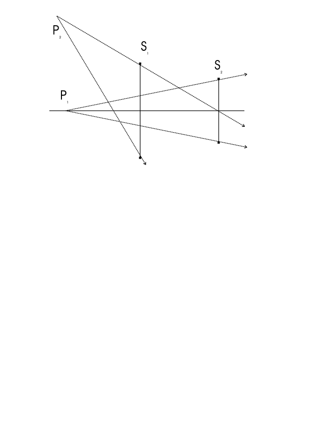
Figure 1: The effect of stops on propagation angles. S₂ is the entrance pupil and object point P₂ is on the edge of the field.

Fig. 1 illustrates the situation described above; object point P₁ is an axis point and obviously stop S₂ is the entrance pupil, responsible for the limitation on the rays that enter the system. According to general practice, we would define the field limits as the points on the rays that pass on the edges of the stop S₁ and the center of the entrance pupil; point P₂ is one such point. Naturally, stop S₁ also introduces limitations on the rays that enter the system, besides its prime function as field limiter; this effect is known as vignetting.

The effect in phase space is illustrated in Fig. 2 where a similar situation is depicted. Fig. 2 a) shows the effect of the entrance pupil on the local WDF with a clipping to its own width. The field pupil, stop S₁, produces its clipping on the WDF back-propagated from the entrance pupil, as shown in Fig. 2 b), and the resulting double-clipped WDF is back-propagated to the scene plane, as shown in Fig. 2 c). The resulting parallelogram shape is the representation in phase space of the signal that can, in fact, enter the system; it is clear that for a point on the axis, $q=0$, the stop S₂ is responsible for determining the admittance angle, while stop S₁ is, to a great extent, responsible for determining the dominion of $q$, which is exactly what we call field. The vignetting effect is visible for extreme values of $q$, for which stop S₂ no longer determines completely the admittance angle.

The extension of the above procedures to a general mapping situation, outside the paraxial approximation, must be done carefully. In the next section we study a complete mapping situation, illustrating both the WDF transformations and stop consideration.

4 Example

The case below was chosen not for its particular applicability but for its ability to demonstrate and highlight the possibilities opened by the matrix mapping and WDF used together.

We will consider a simple imaging system composed of a single convex lens and a field stop on the image plane. The lens was chosen to produce a high degree of aberrations, so that the non-linear effects are clearly visible. The lens is plano-convex, with the flat surface facing the image plane, and has a refractive index of $1.56$; the convex surface has a radius of $6.5\times 10^{-2}~{}\mathrm{m}$ and the central thickness is $2.0\times 10^{-2}~{}\mathrm{m}$. The lens and field stop diameters will be decided later on, upon examination of the aberrations present in the image.

Eqs. (15 to 18) were established for the system in consideration using the method outlined by Almeida [6] using Mathematica [16]. The same software package was also used for all the further calculations. The analysis was carried out on a meridional plane, so the detection of aberration effects such as astigmatism is out of the question. The input scene was defined according to Eq. (3) in terms of its WDF as:

$$W^{i}(q,p)=1+\sin\frac{4\pi q}{l},$$ (23)

where $l$ is a parameter used to control the detail on the scene; all the graphics were plotted with $l=5\times 10^{-2}~{}\mathrm{m}$.

The input scene was located at $13.7\times 10^{-2}~{}\mathrm{m}$, so that the image was formed at $5\times 10^{-2}~{}\mathrm{m}$. Fig. 3 shows the input scene in phase space and the output WDF. The input appears as a series of light and dark bands, showing the independence of the corresponding WDF on the $p$ coordinate, characteristic of spatially incoherent light, a special case of quasi-homogeneous light [1, 3]. The output shows the same bands, reduced in width due to a magnification factor lower than unity and distorted by aberrations. A qualitative analysis of the aberrations is indeed interesting.

The S-shape of the bands results from spherical aberration of various orders, with predominance of the third-order. The reduced width of the bands for higher values of $q$ is characteristic of barrel distortion; this so high that the signal does not exist above $|q|>0.5$, except for the effect of spherical aberration. This is similar to a fish-eye objective. Field curvature is clearly visible as tilting of the central portion of the bands for high $|q|$. Coma results in an asymmetry of the S-shape.

Clearly we have performed a mapping with an infinite diameter lens, which only works mathematically. Considering the radius and width of the curved surface, we have established a lens diameter of $4\times 10^{-2}~{}\mathrm{m}$. The lens diameter was given to a stop located on the vertex plane and the edges of this stop were mapped forward, through the lens and free-space, to the image plane, and backward to the input scene plane. The maps of the lens diameter stop are superimposed on the corresponding WDFs as dashed lines. We decided to use a field stop on the image plane, in order to limit the image to an area of low aberration; a diameter of $4\times 10^{-2}~{}\mathrm{m}$ was also chosen for this stop. The field stop was mapped onto the input scene plane and is shown as a solid line superimposed on both figures. If we were dealing with coherent light the area of both WDFs common to the zones defined by the two stops would be the area relevant for the image formation; in fact, to put it correctly, the image WDF should have been made equal to zero outside that area.

For a one-dimensional stop Eq. (22) becomes [13]

$$S(q)=1-\frac{|q|}{2d}, \rightarrow |q|\leq 2d,$$

$$S(q)=0, \rightarrow |q|>2d.,$$ (24)

where $d$ is the half-width of the stop. So, in incoherent illumination, rather than clipping the local WDF, the stop produces a gradual transition from full intensity to zero with twice the width of the stop. When propagated to either the image or the object planes this transition manifests itself as a gradual transition of the WDF from the full mapped value to zero guided but not delimited by the stops’ traces, see Fig.  4.

5 System analysis

Although not presented in this paper, it would be possible to extract a lot of information about the system from the image WDF modulated by the stops. The field distribution would be obtainable directly from an integration of the image WDF in the variable $p$; the integration limits would be established by maps of stops twice the width of real the stops. It is clear that, within the region delimited by the field stop, there is a reasonable reproduction of the original scene.

The point spread function for an input point $q_{0}$ could be evaluated considering a different input scene, such as $W^{i}(q,p)=\delta(q-q_{0})$, and again integrating the output WDF in $p$. The MTF could also be evaluated using the same scene but performing the integration in $q$.

6 Conclusions

The authors presented a method to evaluate the WDF transformations of an optical signal that passes through a system, in the context of geometrical optics. Using matrices it is possible to model centered systems up to any desired order of approximation; the authors have shown that the same matrix method can be used for the evaluation of the WDF transformations.

The effect of stops and lens diameter could also be accounted for leading to the definition of clipping traces on both the input and output WDF and to the outline of methods to evaluate the resulting field distribution, point spread function and MTF.

7 Acknowledgements

J. B. Almeida wishes to acknowledge the fruitful discussions with P. Andrés, W. Furlan and G. Saavedra at the University of Valencia.

On the occasion of his retirement, this paper is dedicated to Professor K Srinivasa Rao in celebration of his long productive career in theoretical physics.

Figure 2: Effect of stops in phase space. a) Clipping at the entrance pupil, b) the WDF is back-propagated from the entrance pupil to the field pupil and clipped, c) back-propagation to the scene plane.

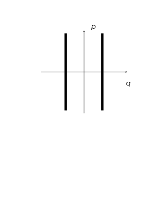
a) b)


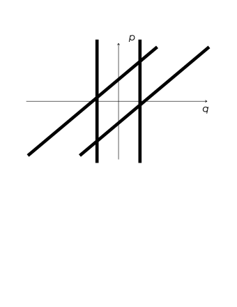
c)

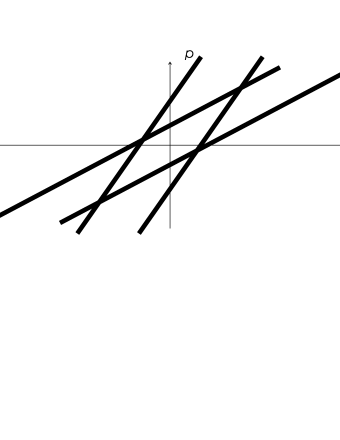
Figure 3: Transformation of the Wigner distribution function through a lens; a) input distribution, b) output distribution. Both figures show the clipping effect of the lens diameter (dashed line) and the field stop (solid line).

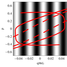
a) b)

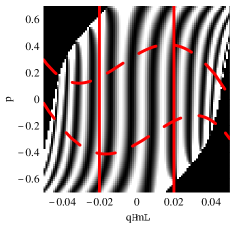
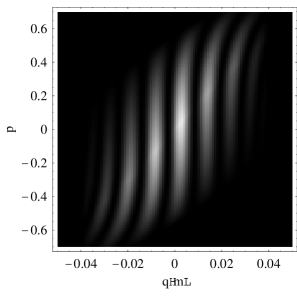
Figure 4: The Wigner distribution function on the image plane shows the effect of stops. With incoherent illumination the stops don’t clip the distribution but apply a smoothing from the center of the stop to twice the stop width.

References

- [1] M. J. Bastiaans, “The Wigner Distribution Function Applied to Optical Signals and Systems,” Opt. Commun. 25, 26–30 (1978).
- [2] D. Dragoman, “The Wigner Distribution Function in Optics and Optoelectronics,” in Progress in Optics, E. Wolf, ed., (Elsevier, Amsterdam, 1997), Vol. 37, Chap. 1, pp. 1–56.
- [3] M. J. Bastiaans, “Application of the Wigner Distribution Function in Optics,” In The Wigner Distribution - Theory and Applications in Signal Processing, W. Mecklenbräuker and F. Hlawatsch, eds., pp. 375–426 (Elsevier Science, Amsterdam, Netherlands, 1997).
- [4] M. J. Bastiaans, “The Wigner Distribution Function and Hamilton’s Characteristics of a Geometric-Optical System,” Opt. Commun. 30, 321–326 (1979).
- [5] M. J. Bastiaans, “Second-Order Moments of the Wigner Distribution Function in First-Order Optical Systems,” Optik 88, 163–168 (1991).
- [6] J. B. Almeida, “General Method for the Determination of Matrix Coefficients for High Order Optical System Modeling,” J. Opt. Soc. Am. A 16, 596–601 (1999).
- [7] K. Riley, M. P. Hobson, and S. J. Bence, Mathematical Methods for Physics and Engineering (Cambridge University Press, Cambridge, U. K., 1998).
- [8] M. Kondo and Y. Takeuchi, “Matrix Method for Nonlinear Transformation and its Application to an Optical Lens System,” J. Opt. Soc. Am. A 13, 71–89 (1996).
- [9] V. Lakshminarayanan and S. Varadharajan, “Expressions for Aberration Coefficients Using Nonlinear Transforms,” Optom. Vis. Sci. 74, 676–686 (1997).
- [10] M. Born and E. Wolf, Principles of Optics, 6th. ed. (Cambridge University Press, Cambridge, U.K., 1997).
- [11] J. B. Almeida and V. Lakshminarayanan, “Position and Shape Dependence of the Eye’s Entrance Pupil on Eccentricity Angle,” In ICO XVIII, 18th Congress of the International Commission of Optics, Proc. SPIE 3749, 631–632 (S. Francisco, USA, 1999).
- [12] “Oslo LT – Version 5,”, Sinclair Optics, Inc., 1995, optics design software.
- [13] J. W. Goodman, Introduction to Fourier Optics (McGraw-Hill, New York, 1968).
- [14] J. B. Almeida and V. Lakshminarayanan, ”Wide Angle Near-Field Diffraction and Wigner Distribution”, Submitted to Opt. Lett. (unpublished).
- [15] M. J. Bastiaans and P. G. van de Mortel, “Wigner Distribution of a Circular Aperture,” J. Opt. Soc. Am. A 13, 1699–1703 (1996).
- [16] “Mathematica 4.0,”, Wolfram Research, Inc., 1999.
a)  b)
b)
c)
a)  b)
b)