Multiscale Trend Analysis

Abstract

This paper introduces a multiscale analysis based on optimal piecewise linear approximations of time series. An optimality criterion is formulated and on its base a computationally effective algorithm is constructed for decomposition of a time series into a hierarchy of trends (local linear approximations) at different scales. The top of the hierarchy is the global linear approximation over the whole observational interval, the bottom is the original time series. Each internal level of the hierarchy corresponds to a piecewise linear approximation of analyzed series. Possible applications of the introduced Multiscale Trend Analysis (MTA) go far beyond the linear interpolation problem: This paper develops and illustrates methods of self-affine, hierarchical, and correlation analyses of time series.

Key words: multiscale trend analysis, piecewise linear approximation, hierarchical scaling.

1 Introduction

The motivation for the Multiscale Trend Analysis (MTA) introduced in this paper is to describe and analyze time series in terms of their observed trends (local linear approximations). Indeed, trends are the most intuitive feature of a time series and it seems natural to use them for series quantitative description. Such a description is intrinsically multiscale since each non-trivial process exhibits juxtaposition of trends of different duration and steepness depending on the observational scale.

The proposed analysis is based on piecewise linear approximations of the analyzed time series. Construction of such approximations involves a tradeoff between quality and detail. We formulate (see Sect. 2.3) a local optimality criterion and use it in a multiscale fashion to detect local trends in a time series at all possible scales, thus forming a hierarchy of trends. This hierarchy serves as a unique representation of the original time series and is used for quantitative analysis.

The problem of piecewise interpolation of time series has been given significant attention in the context of image processing (see for example [1, 2, 3]). However, the focus was on constructing an optimal piecewise linear approximation $L_{\epsilon}(t)$ with minimal number of segments for given error $\epsilon$ (deviation from the original signal). On the contrary, we concentrate on finding a whole hierarchy of consecutively more detailed approximations.

This paper illustrates the following applications of MTA:

• Descriptive and exploratory data analysis. Computationally effective trend decomposition naturally complements a standard data miner’s toolbox. Conveniently, MTA does not rely on any assumptions about the analyzed time series (e.g. stationarity or existence of higher moments) while its results are easily interpreted

• Self-affine analysis. Particularly, MTA provides a way to extract local fractal properties of the processes.

• Hierarchical analysis. Representation of a time series as a hierarchy (tree) allows one to use methods borrowed from the theory of hierarchical scaling complexities [4]. Particularly, Horton-Strahler indexing provides a natural way to consider scaling laws for trends.

• Correlation analysis. MTA allows one to detect non-linear correlations, particularly those caused by the presence of amplitude modulation and non-linear long-term trends.

The paper is organized as follows: Section 2 introduces the basic notions and describes the computational algorithm for decomposition of a series into a hierarchy of trends. Methods of MTA-based self-affine analysis comprise Sect. 3. Section 4 introduces hierarchical analysis of time series. Correlation analysis is described in Sect. 5. Fractional Brownian walks and Mandelbrot cascade measures are used to illustrate methods of Sect. 3 - 5. Section 6 concludes.

2 Multiscale Trend Decomposition

The core of the MTA is construction of a hierarchical tree $T_{X}$ that describes the trend structure of a given time series $X(t)$ . Trend is defined here as a linear least square approximation of $X(t)$ at a subinterval of the observational time interval. The tree $T_{X}$ is formed step-by-step, from the largest to the smallest scales: First, we determine the longer trends, then look for the shorter and shorter trends against the background of already established ones, all the way down the hierarchy of scales. The larger the scale at which the trend is observed, the higher the level of the corresponding vertex within the tree. The root (top vertex) of the resulting tree $T_{X}$ corresponds to the global linear trend of $X(t)$; each internal vertex corresponds to a distinct local trend, the leaves (vertices with no descendants) to the the elementary linear segments of the original time series $X(t)$: $\left[X(t_{i}),X(t_{i+1})\right]$. The union of leaves thus coincides with $X(t)$.

A recursive procedure for constructing the tree $T_{X}$ is described below.

2.1 Scheme of the decomposition

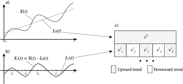
Figure 1: Scheme of the Multiscale Trend Decomposition. a) At zero step $X(t)$ is approximated by its global linear trend $L_{0}(t)$. b) Detrended series $X_{1}(t)=X(t)-L_{0}(t)$ is approximated by the piecewise linear function $L_{1}(t)$, the whole analysis is then repeated at each of subintervals $[t_{i}^{1},~{}t_{i+1}^{1}]$. c) Resulting hierarchy of trends. See Sect. 2 for details.

Without loss of generality we presume that the time series $X(t)$ is observed at a finite number of epochs within the time interval $[0,~{}1]$. At the first step the whole time series $X(t),~{}t\in[0,~{}1]$ is approximated by a single trend — the linear least square fit $L_{0}(t)$ (Fig. 1a).

This trend forms the vertex $v^{0}$ at the level 0 (the root) of the resulting hierarchical tree $T_{X}$ (Fig. 1c). It is also convenient to say that the root of $T_{X}$ corresponds to the whole time interval $[0,~{}1]$, and vice versa. At the next step we determine secondary trends on the background of the first global one. For this we consider the deviation $X_{1}(t)=X(t)-L_{0}(t),~{}t\in[0,~{}1]$ of $X(t)$ from its linear trend $L_{0}(t)$ and approximate it by a piecewise linear (discontinuous) function $L_{1}(t)$ (Fig. 1b). The most delicate part of the analysis — choosing the optimal number $n^{0}$ of segments for this approximation — is described below in Sect. 2.2. The approximation $L_{1}(t)$ results in partition of the time interval $[0,~{}1]=I^{0}$ into $n^{0}$ nonoverlapping subintervals $I^{1}_{i}=[t^{1}_{i},~{}t^{1}_{i+1}],~{}i=1,\dots,n^{0}$, with $t^{1}_{1}=0$, $t^{1}_{n^{0}+1}=1$. The linear segments $l^{1}_{i}(t)$ that comprise $L_{1}(t)$ are determined by the least square fit of $X(t)$ within corresponding subintervals. They form $n^{0}$ vertices $v_{i}^{1},~{}i=1,\dots,n^{0}$ at level 1 of the tree $T_{X}$. The enclosures $I^{1}_{i}\subset I^{0}$ are reflected in the structure of the tree $T_{X}$ by the fact that the vertices corresponding to subintervals $I^{1}_{i}$ are descendants of the root, which corresponds to $I^{0}$.

Repeating the above procedure at arbitrary interval $I_{i}^{1}$ from level 1 we form $n^{1}_{i}$ ternary linear trends, each determined by the least square fit of $X(t)$ at a subinterval $I^{2}_{j}\subset I^{1}_{i}$, $j=1,\dots,n^{1}_{i}$. The union of $N_{2}=\sum_{i=1}^{n^{0}}n_{i}^{1}$ such trends descending from all the trends of level 1 form level 2 of the tree $T_{X}$. To index the vertices (local trends) at level 2 we use the natural ordering induced by the corresponding time partition: $v^{2}_{i}$ ($l^{2}_{i}$) denotes the vertex (trend) that corresponds to the time subinterval $I^{2}_{i}=\left[t^{2}_{i},~{}t^{2}_{i+1}\right]$, $i=1,\dots,N_{2}$.

Repeating the same procedure at each time interval of level $l$, $l\geq 0$ we form level $(l+1)$. It consists of

$$N_{l}=\sum_{i=1}^{N_{l-1}}n^{l-1}_{i}$$

subintervals (vertices). By construction, $N_{0}=1$ and $N_{k}<N_{p}$ for $k<p$. We depth of the resulting tree is denoted by $L$.

Each level $l$ of the tree $T_{X}$ corresponds to a piecewise linear approximation $L_{l}(t)$ of the time series $X(t)$ as well as to the induced partition $I^{l}=\left\{I^{l}_{i},~{}i=1,\dots,N_{l}\right\}$ of the observational interval $I^{0}$. The global piecewise linear approximation $L_{l}(t)$ at level $l$ is a union of local linear approximations $l^{l}_{i}(t)$, $t\in I^{l}_{i}=\left[t^{l}_{i},~{}t^{l}_{i+1}\right]$, $i=1,\dots,N_{l}$, and $I^{0}=\cup_{i=1}^{N_{l}}I^{l}_{i}~{}\forall l$.

By $r^{l}_{i}$ we denote the length of subinterval $I^{l}_{i}$, and by $e^{l}_{i}$ the rms deviation of $X(t)$ from its linear fit $l^{l}_{i}(t)$ at this subinterval:

$$e^{l}_{i}=\sqrt{\sum_{t\in I^{l}_{i}}\left(\vphantom{{}^{I}}X(t)-l^{l}_{i}(t)\right)^{2}}.$$ (1)

The total fitting error $E_{l}$ at the level $l$ is given by

$$E_{l}^{2}=\sum_{i=1}^{N_{l}}\left(e^{l}_{i}\right)^{2}=\sum_{t\in I^{0}}\left(\vphantom{{}^{I}}X(t)-L_{l}(t)\right)^{2}.$$ (2)

All vertices (subintervals) at a given level of $T_{X}$ result from the same number of divisions of the initial interval $[0,~{}1]$. However, in many applications it is desirable to work with approximations characterized by a similar scale of observed trends, independently of the division history. To take this into account we consider the modified tree $M_{X}$ obtained from $T_{X}$ by the following procedure. The first two levels of $M_{X}$ are the same as that of $T_{X}$. Each consecutive level is formed by division of only one of the existing subtrends and leaving all the other unchanged. A subtrend $v_{i}^{l}$ to be divided corresponds to the maximal improvement of the fitting quality $\Delta=\left(e_{i}^{l}\right)^{2}-\sum\left(e_{c}^{l+1}\right)^{2}$, where $c$ runs over the indexes of children of the vertex $i$. We will call $T_{X}$ the topological and $M_{X}$ the metric tree associated with the series $X(t)$. To avoid excessive notations we will use the same indexing for both the trees $T_{X}$ and $M_{X}$ stating each time which one is considered.

2.2 Optimal piecewise linear approximation

Here we describe a procedure for finding the optimal piecewise linear approximation $L(t)$ of a series $X(t)$ at a given time interval. Without loss of generality we suppose that the interval is $[0,~{}1]$. The problem, of course, is in finding the optimal tradeoff between the number $N$ of linear segments within $L(t)$ and the corresponding fitting quality $E$. Clearly, the larger the number $N$, the better the resulting fit. Our goal is to depict by linear segments only the most prominent large-scale trends of $X(t)$ leaving the smaller fluctuations for the later steps of the decomposition. To solve this problem we employ the function

$$H(N,E)=-\frac{\log(E/E_{0})}{N-1},$$ (3)

where $E_{0}$ is the fitting error of the global linear approximation $L_{0}(t)$ of $X(t)$ on $[0,~{}1]$. This function measures the quality of a piecewise linear approximation $L(t;N,E)$ which consists of $N$ linear segments and has total fitting error $E$. The optimal approximation $L(t;N^{*},E^{*})$ corresponds to the maximum of $H(N,E)$:

$$H(N^{*},E^{*})=\max_{N,E}H(N,E).$$ (4)

Geometrically, consider the plane $\left(N,\log(E/E_{0})\right)$, $N$ being the number of linear segments within a piecewise linear approximation of $X(t)$ on $[0,~{}1]$, and $E$ the total fitting error. The global linear approximation $L_{0}(t)$ at the whole interval $[0,~{}1]$ corresponds to the point $p_{0}=(1,0)$. An arbitrary piecewise approximation $L_{i}(t)$ corresponds to the point $p_{i}=(N_{i},\log(E_{i}/E_{0}))$, $N_{i}\geq 1$, $E_{i}\leq E_{0}$. The slope of the linear segment $[p_{0},p_{i}]$ shows the increase of the fitting quality per one additional segment of approximation. By the criterion (3,4) we chose the approximation with the maximal quality increase.

With the above criterion (3,4) one can find the optimal approximation by a full search over all possible partitions of $[0,~{}1]$ by epochs of $X(t)$ into $N=2,3,...$ subintervals. However, the computational complexity of such an approach depends exponentially on the number of observations so it can hardly be used in practice. In Sect. 2.3 below we introduce an optimized search based on the idea that partition epochs should correspond to the prominent edges of the analyzed series $X(t)$.

2.3 Optimized search

The idea of the optimized search is to reasonably reduce the set of possible partition epochs by considering only those at which $X(t)$ significantly changes its slope — edge points.

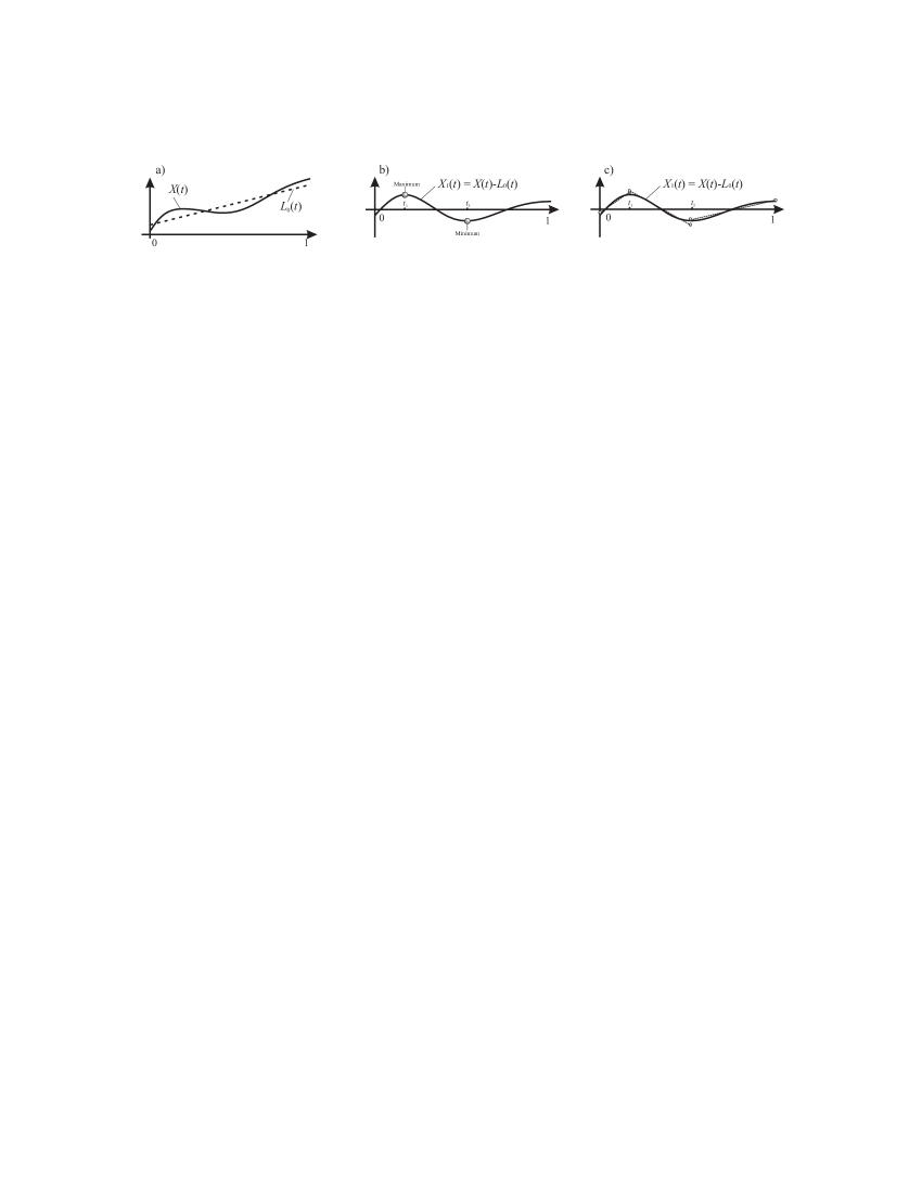
Figure 2: Scheme of detection of edge points. a) At zero step $X(t)$ is approximated by its global linear trend $L_{0}(t)$. b) Epochs $(t_{1},t_{2})$ of global maximum and minimum of the detrended series $X_{1}(t)=X(t)-L_{0}(t)$ are located. c) Analysis is repeated at each of subintervals $[0,t_{1}]$, $[t_{1},t_{2}]$, and $[t_{2},1]$.

The edge points are determined by the following recursive procedure illustrated in Fig. 2.

At the first step we choose the epochs $(t_{1},t_{2})$ corresponding to the maximum and minimum of the detrended function $X_{1}(t)=X(t)-L_{0}(t)$, where $L_{0}(t)$ is a least-square linear fit of $X(t)$ in $[0,~{}1]$. If one of these epochs coincides with the interval boundary (say, $t_{1}=0$) only the remaining epoch ($t_{2}$) is considered. If both these epochs coincide with the interval boundaries, we redefine $L_{0}(t)$ as the line connecting $X(0)$ and $X(1)$ and repeat the procedure. As a result we have one or two partition epochs within the initial interval; they divide it into two or three subintervals respectively. The procedure is now repeated for each of these subintervals, producing two to six new partition epochs. Together with already selected ones, they divide the initial interval into, respectively, four to nine subintervals, etc. The partition stops when the predefined number $(N_{h}-1)$ of partition epochs is collected; this corresponds to $N_{h}$ subintervals.

With $(N_{h}-1)$ possible partition epochs there are $\left(2^{N_{h}-1}-1\right)$ ways to divide the interval into $2,\dots,N_{h}$ subintervals. The optimal — according to (3,4) — partition can be found by $\left(2^{N_{h}-1}-2\right)$ operations.

To further reduce the computation volume, we first choose the optimal one from $(N_{h}-1)$ partitions formed by $(N_{h}-2)$ partition epochs. Next, only the $(N_{h}-2)$ epochs that form this partition are used to find the optimal partition with $(N_{h}-3)$ partition epochs, etc. Finally, we use criterion (3,4) to choose the optimal from $(N_{h}-1)$ partitions, each having a distinct number of subintervals ranging from $2$ to $N_{h}$. This way we reduce the number of operations to $(N_{h}^{2}-N_{h}-2)/2$.

Clearly, the above optimization may produce a piecewise function which does not coincide with the optimal one resulting from applying the criterion (3,4) to the whole variety of possible partitions. As such, this optimization should be considered as a computationally effective approximation of the result. Extensive numerical experiments show that it is reasonably good for a wide range of time series including fractional Brownian motions with different Hausdorff measures and self-affine processes coming from geophysical observations.

2.4 Examples

Here we show some examples and illustrate different ways to visualize the results of the decomposition.

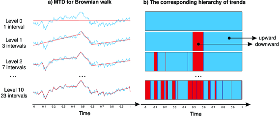
Figure 3: Decomposition of a Fractional Brownian walk with Hausdorff measure $Ha=0.7$. a) Piecewise linear approximations at levels $l=0,1,2,10$. b) Corresponding hierarchical tree.

Figure 3 shows four levels, $l=0,1,2$, and $10$ of tree $M_{X}$ for a fractional Brownian walk with Hausdorff measure $Ha=0.7$. Panel a) shows the analysed series $X(t)$ and the piecewise linear approximations $L_{l}(t),~{}l=0,1,2,10$, while panel b) shows the four corresponding levels of the tree $M_{X}$.

One can see how the fitting quality improves with the number of linear segments: each consecutive approximation tries to account for the most prominent variations of $X(t)$ adding the least possible number of new segments. For example, starting with the three segments of the decomposition $L_{1}(t)$ at level 1, it is clearly more efficient to improve the leftmost segment, which exhibits large deviations around $t=0.1$, than work with the central or rightmost one. When work is done with the largest deviation (see level 2) we proceed to the smaller ones.

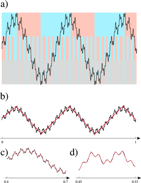
Figure 4: Decomposition of the sum of three sinusoids, $X(t)=\sin(5\pi t)+\frac{1}{5}\sin(60\pi t)+\frac{1}{10}\sin(200\pi t)$. a) $X(t)$ on the background of three levels from its decomposition. b) Piecewise linear approximation corresponding to the top level of the decomposition shown in panel a). c) Fragment corresponding to the middle level of a). d) Fragment corresponding to the bottom level of a).

The function shown in Fig. 4a on the background of its tree $M_{X}$ is a sum of three sinusoids with different frequencies.

The amplitudes are chosen in such a way that the largest fluctuations are carried at the smallest frequency, intermediate at the second largest, and smallest at the highest one. This structure is clearly depicted by the decomposition with each separate level responsible for a distinct frequency (see panels b), c), and d)).

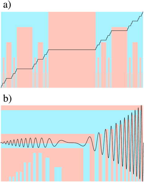
Figure 5: Decomposition of a) Devil’s Staircase (5 upper levels of $M_{X}$ are shown) and b) modulated sinusoid with time-dependent frequency (15 levels are shown).

Two more examples are given in Fig. 5 where we show only the signals $X(t)$ and the upper levels of their trees $M_{X}$, which is enough to understand the shape of corresponding piecewise linear approximations. Decomposition for the famous Devil’s Staircase is shown in Fig. 5a: it gives the exact description of the staircase structure. Figure 5b shows a decomposition for modulated oscillations with time-dependent frequency. Contrary to the panel a) here we use color-code to depict slope changes (from downward to upward or vice versa), not their directions. In this example one can see how the amplitude of oscillation is reflected in the decomposition: the higher the amplitude, the higher the level at which it is first detected.

2.5 On the numerical parameter $N_{h}$

The only numerical parameter of our algorithm is the maximal number $N_{h}$ of secondary trends (see Sect. 2.3). Large values of $N_{h}$ contribute to the computational complexity, while small values may prevent fast detection of optimal approximation and create superfluous levels of the hierarchy $T_{X}$. Numerous experiments suggest the value $N_{h}=5$ as the optimal tradeoff, and we use it for all experiments presented in this paper.

Clearly, with $N_{h}=5$ we are not insured from creating unnecessary levels. For example the division of Fig. 4b consists of 6 ($>N_{h}=5$) linear segments, so it could not be obtained by a single division of the original series. In fact this is level 2 of the original hierarchy $M_{X}$. Analogously, the intermediate division of Fig. 4a (see also Fig. 4c) corresponds to level 19, and the bottom one (Fig. 4d) to level 82.

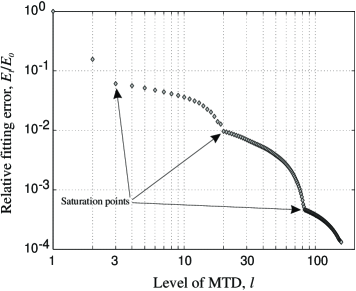
Figure 6: Illustration of removing unnecessary levels from the decomposition (for the signal shown in Fig. 4). Prominent saturation points correspond to the three levels shown in Fig. 4

The simple procedure used to remove unnecessary levels is illustrated in Fig. 6 where we show the fitting error $E_{l}/E_{0}$ for all levels $l$ of the tree $M_{X}$ constructed for the signal of Fig. 4a. The prominent edge points show the three levels at which saturation of the fitting quality is reached; only these three levels are left in Fig. 4a.

If the analyzed tree has only less-than-5-fold partitions (which is the case for the Devil’s Staircase of Fig. 5a) the above procedure is unnecessary. The properties of this procedure and conditions for its use are beyond the scope of the present paper.

3 Self-affine analysis

In this section we demonstrate how self-affine properties of a time series are reflected in its decomposition $M_{X}$.

Recall [5, 6] that statistical properties of a self-affine time series $X(t)$ remain the same under the transformation

$$\left\{\begin{array}[]{lcl}t^{\prime}&=&rt,\\ X^{\prime}&=&r^{Ha}X.\end{array}\right.$$ (5)

That is, when one changes the observational time scale by a factor of $r$, the scale of measurements should be changed by a factor of $r^{Ha}$ in order to preserve the characteristic statistical features of $X(t)$. The parameter $Ha$ is called Hausdorff measure; it is related to the fractal dimension $D$ of a self-affine time series as $Ha=2-D$ [6]. Accordingly, for one-dimensional time series the Hausdorff measure may take values within the range $0<Ha<1$. A useful interpretation of $Ha$ comes from the character of correlations between the time series increments: $\Delta_{i}=X(t_{i})-X(t_{i-1})$. Negative correlations between $\Delta_{i}$ and $\Delta_{i+1}$ lead to high fluctuations of $X(t)$ and as a result to absence of pronounced trends; this situation corresponds to small values of Hausdorff measure: $Ha<1/2$. Positive correlations — leading to existence of long-term trends — correspond to $Ha>1/2$. For a process with independent increments (e.g. Brownian walk) one has $Ha=1/2$.

To estimate the Hausdorff measure of observed time series one typically considers the dependence of a convenient measure of its variation on the length of a corresponding observational interval [5, 6]. In our case the appropriate variation measure can be chosen as the fitting error $E_{l}$ (2) of $M_{X}$ at level $l$. According to (5), for a self-affine series $X(t)$ we expect to observe a power-law relation

$$\frac{E_{l}}{E_{0}}=N_{l}^{-Ha}=R_{l}^{Ha},$$ (6)

where $N_{l}$ is the number of segments at the level $l$, $R_{l}=N_{l}^{-1}$ is their mean length.

As a model example we consider fractional Brownian walks (FBWs) with Hausdorff measures in the range $0<Ha<1$.

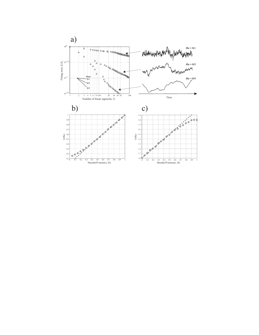
Figure 7: Relation between Hausdorff measure and error scaling for fractional Brownian walks (FBW). a) Trajectories of FBWs with $Ha=0.1,0.5,0.9$ and corresponding error scalings. b) Relation $b(Ha)$ for FBWs, $0\leq Ha\leq 1$, values of $b$ averaged over 100 realizations of FBW for each value of $Ha$. c) The same as b) for integrated FBWs.

Figure 7a shows trajectories and the corresponding $(N_{l},E_{l})$-scalings for three FBWs with $Ha=0.1,0.5,$ and $0.9$. Figure 7b shows the value $b(Ha)$ estimated by the best linear square fit from the relation

$$\log(E_{l}/E_{0})=-b\log(N_{l})$$ (7)

based on decomposition of 2100 independent FBWs; to remove statistical fluctuations we averaged $b$ over 100 FBWs for each value of $Ha$. As seen in Fig. 7b, the scaling (6) clearly holds for $Ha>0.3$; the deviations observed at the smaller values of $Ha$ are due to the fact that the corresponding FBWs become noisier and hardly display pronounced trends. This effect is typical for self-affine analysis (e.g., see [7]). To neglect it we consider the integrated signal $Y(t)=\sum_{s\leq t}X(s)$. Estimations of the slope $b(Ha)$ for integrated FBWs are presented in Fig. 7c. The linear relation $b(Ha)=Ha+1$ is now observed for $0<Ha<0.6$, the change of slope compared to Fig. 7b is due to the integration procedure.

Another way to estimate $Ha$ is to consider the error-length dependence for all individual linear segments comprising $M_{X}$:

$$\frac{e^{l}_{i}}{E_{0}}=\left(r^{l}_{i}\right)^{Ha+1/2},~{}l=1,\dots,L,~{}i=1,\dots,N_{l}.$$ (8)

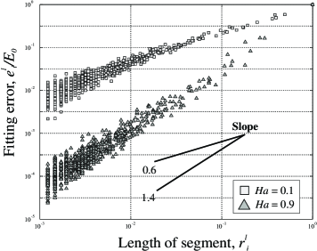
Figure 8: Error-length dependence for individual vertices of trees $M_{X}$ corresponding to FBW with $Ha=0.1,0.9$. The scaling (8) is clearly observed.

The difference in the power exponents of relations (6) and (8) is explained by the fact that the former deals with averaged statistics, while the latter deals with characteristics of individual intervals. Figure 8 illustrates the error-length dependence (8) for FBWs with $Ha=0.1$ and $Ha=0.9$.

Importantly, MTA provides a convenient basis for estimation of local Hausdorff measures $Ha(t)$. Consider all the intervals from $T_{X}$ that cover epoch $t$. At each level $l$ of $T_{X}$ there is one and only one such interval; we use the index ${}^{l}_{(t)}$ to denote this interval and all its characteristics. The local Hausdorff measure $Ha(t)$ is estimated now from the relation

$$\frac{e^{l}_{(t)}}{E_{0}}=\left(r^{l}_{(t)}\right)^{Ha(t)+1/2},~{}l=1,\dots,L.$$ (9)

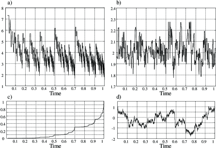
Figure 9: Estimation of local Hausdorff measures, $Ha(t)$ for a multifractal (Mandelbrot cascade measure) (panel a) and monofractal (Brownian walk) (panel b). Corresponding time series are shown in panels c) (multifractal) and d) (monofractal).

Figures 9a,b show the dynamics of the local Hausdorff measure for multi- and monofractals. We use a Mandelbrot cascade measure $M(0.7,0.3;0.3,0.7)$ as a model example of a multifractal (Fig. 9c), and a Brownian walk as that of a monofractal (Fig. 9d). The definition of Mandelbrot cascade measure is given in Appendix A. Note that the range of $Ha(t)$ variation for the monofractal (Fig. 9b) is an order of magnitude less than that for the multifractal (Fig. 9a).

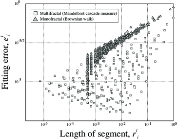
Figure 10: Error-length dependence for multi- and monofractals of Fig. 9. Note that the point scattering is significantly larger for the multifractal.

The points $\left(e^{l}_{(t)},~{}r^{l}_{(t)}\right)$ used in (9) to estimate the local Hausdorff measure are extracted from the whole set $\left(e^{l}_{i},~{}r^{l}_{i}\right)$ of (8). This suggests a method for detecting multifractality in $X(t)$: the larger the scattering of the points $\left(e^{l}_{i},~{}r^{l}_{i}\right)$, the larger the probability that the observed series is a multifractal. Formal statistical tests can be easily constructed from this general principle based on the particular problem at hand. The character of temporal variations of $Ha(t)$ (Figs. 9a,b) can be also used in such tests. An example of the scattering $\left(e^{l}_{i},~{}r^{l}_{i}\right)$ is shown in Fig. 10 for mono- and multifractals of Fig. 9. In this model example the difference is obvious.

4 Hierarchical scaling

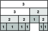
Figure 11: Horton-Strahler indexing.

The appropriate ordering of vertices within a tree $T_{X}$ is very important for meaningful description and analysis of the series $X(t)$. The problem of such an ordering becomes not trivial as soon as the tree is not uniform (i.e. is not formed by applying the same deterministic division rule to each of its vertices). A befitting way to solve this problem is given by the Horton-Strahler topological classification of ramified patterns [4, 8, 9] illustrated in Fig. 11: One assigns orders to the vertices of the tree, starting from $k=1$ at leaves (vertices with no descendants).

The order of an internal vertex equals the maximal order $m$ of its descendants, if they are distinct, and $m+1$ if they are all equal. Originally introduced in geomorphology by Horton [8] and later refined by Strahler [9], this classification is shown to be inherent in various geophysical, biological, and computational applications [4, 10, 11, 12].

As a result of the Horton-Strahler indexing of the tree $T_{X}$, each of its vertices is characterized by an order $k$, length $r$ of the corresponding partition interval, and the error $e$ of the linear least square fit of $X(t)$ on this interval. The scaling behavior of $X(t)$ can be described by the exponents of the relations:

$$N(k)\sim 10^{-B_{N}k};~{}R(k)\sim 10^{B_{R}k};~{}E(k)\sim 10^{B_{E}k}.$$ (10)

Here $N(k)$ is the number of vertices of order $k$, $R(k)$ and $E(k)$ are the values of $r$ and $e$ averaged over the vertices of order $k$.

The relation between the number $N(k)$ of vertices of order $k$ and their average length $R(k)$ determines the fractal dimension $d$ of the tree $T_{X}$ [10]:

$$N(k)=R(k)^{-d}.$$ (11)

Combining (10) and (11) we find:

$$d=\frac{B_{N}}{B_{R}}.$$ (12)

The structure of the tree $T_{X}$ can be considered at different levels of detail: First, one can consider only the topological structure (Fig. 12a), where the position of each vertex is uniquely determined by its parent (the nearest vertex placed closer to the root); and any permutation of siblings (the vertices with the same parent) does not change the tree. Each vertex is characterized by its Horton-Strahler index, and the only constraint on a tree resulting from MTA is the maximal possible number $N_{h}$ of siblings, that is subtrends within a given trend. Next, one can add the information on interval partition (Fig. 12b): The siblings become ordered according to the partition of the interval corresponding to their parent. Each vertex $v_{i}$ is additionally characterized by the length $r_{i}$ and the following conservation law holds:

$$r_{i}=\sum r_{c},$$ (13)

where $c$ runs over the indexes of the children of the element $i$.

Finally, (Fig. 12c) one considers error characteristics $e_{i}$, which describe the quality of the linear fit of $X(t)$ within the corresponding time interval. In terms of these errors the system becomes dissipative:

$$e_{i}\geq\sum e_{c},$$ (14)

with the same meaning of subindexes as in (13).

The exponents $B_{N,R,E}$ of (10) reflect different statistical properties of the tree $T_{X}$: $B_{N}$ describes its topological structure while $B_{R}$ and $B_{E}$ relate to the metric structures based, respectively, on properties of interval partition ($r$-metric) and piecewise linear fit ($e$-metric).

For illustration we again use FBWs with different Hausdorff measures.

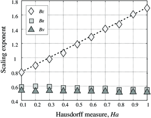
Figure 13: Dependence of scaling exponents $B_{E,R,N}$ (Eq. (10)) on the Hausdorff measure $Ha$ of FBWs. Dashed line is $B=0.7+Ha$.

Figure 13 shows the dependence of the exponents $B_{N,L,E}$ on the Hausdorff measure $0\leq Ha\leq 1$. The estimations are averaged over 100 FBWs for each value of $Ha$. The exponents $B_{N}$ and $B_{R}$ are nearly constant: $B_{N}\approx 0.52$, $B_{R}\approx 0.57$, while for the exponent $B_{E}$ we observe the linear dependence:

$$B_{E}=0.7+Ha\approx\log_{10}(5)+Ha.$$ (15)

These results have an important interpretation: All FBWs with Hausdorff measure in the range $0\leq Ha\leq 1$ have the same topological and $r$-metric structures in terms of MTA tree $T_{X}$. Particularly, trees $T_{X}$ corresponding to different $Ha$ have the same fractal dimension $d=B_{N}/B_{R}\approx 0.9$. The only characteristic that depends on the Hausdorff measure is the fitting error ($e$-metric), that is the degree of variation of $X(t)$ within a given interval.

5 Correlation analysis

One of the important applications of MTA is correlation analysis of time series. The major drawback of classical correlation analysis is that interpretation of its results may be completely ruined by the presence of long-term trends and/or modest amplitude modulations of signals. The MTA can naturally avoid these problems by depicting the essential local properties of the analyzed series.

We start this section by introducing two measures of similarity for time series. One is based solely on the time interval partition induced by $M_{X}$; another takes into account the directions (upward vs. downward) of local trends.

5.1 Distance between partitions

Each level $l$ of the tree $M_{X}$ (Sect. 2) corresponds to a partition of the time interval $[0,~{}1]$ into $N_{l}$ nonoverlapping subintervals. Since each of these subintervals corresponds to a distinct observed trend of the series $X(t)$, the problem of comparison of two such partitions naturally arises. Below we introduce the distance between two partitions.

Consider the space $\Omega$ of finite partitions of the unit interval $[0,~{}1]$. Each partition $A$ is defined by a finite number $n_{A}$ of points; the boundaries $0$ and $1$ are included in all partitions:

$$A=\{0=a_{0}<a_{1}<\dots<a_{n_{A}}<a_{n_{A}+1}=1\}.$$

The trivial partition $U$ consists only of boundary points: $U=\{0,~{}1\}$.

For $A,B\in\Omega$ we say that $B$ is a subpartition of $A$ ($B\subset A$) if all points from $A$ are among points from $B$; this imposes a partial order on $\Omega$. A union $A\cup B$ is defined as the partition consisting of the points included in either $A$ or $B$, without repetitions. An intersection $A\cap B$ is defined as the partition consisting of points included in both $A$ and $B$.

An asymmetric distance $m(A,B)$ from $A$ to $B$ ($A,B\in\Omega$) can be defined as

$$m(A,B)=\sum_{i=1}^{n_{A}}\min_{0\leq j\leq n_{B}+1}\{|a_{i}-b_{j}|\},$$ (16)

which gives for the trivial partition

$$m(A,U)\equiv m(A)=\sum_{i=1}^{n_{A}}\min\{a_{i},1-a_{i}\}$$

The distance (16) is interpreted as the minimal correction to $A$ that makes $B$ its subpartition: $B\subset A^{\prime}$, where $A^{\prime}$ stands for the corrected version of A.

The following properties of $m(A,B)$ follow directly from the definition (16):

1. $0\leq m(A,B)<\infty$;

2. $m(A,B)=0$ iff $B\subset A$;

3. Additivity with respect to $A$: $m(A_{1}\cup A_{2},B)=m(A_{1},B)+m(A_{2},B)$;

4. Monotonicity with respect to $B$ (the triangle inequality): $m(A,B_{1}\cup B_{2})\leq m(A,B_{1})+m(A,B_{2})$.

It is convenient to consider the symmetric function

$$\mu(A,B)=\max\{m(A,B),m(B,A)\},$$ (17)

whose small values signal that the partitions $A$ and $B$ are similar. Note that $\mu$ is not a distance since it does not satisfy the triangle inequality. The reciprocal $\mu^{-1}$ may serve as a measure of partition correlation.

5.2 Slope sign correlation

Here we introduce the correlation function that describe similarity between two piecewise linear approximations $L^{1}(t)$ and $L^{2}(t)$ of $X(t),~{}t\in[0,~{}1]$. (We use upper indexes in order not to mix these arbitrary approximations with $L_{1}(t)$, and $L_{2}(t)$ at the first and second levels of the decomposition.) This correlation function is based on the coarse information about trends from $L^{i}(t)$: We take into account only their directions — upward vs. downward.

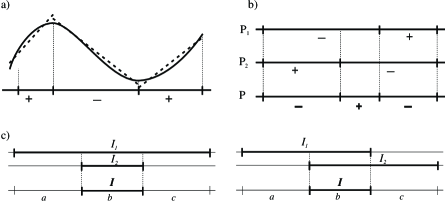
Figure 14: Signed partition corresponding to a piecewise linear approximation (panel a), union of signed partitions (panel b), and triplet $(a,b,c)$ for an interval of a union of partitions. see Sect. 5.2.

First, we introduce the signed partitions $P_{1}$ and $P_{2}$ of the interval $[0,~{}1]$. They are formed by the intervals of constant sign of the slope of $L^{i}(t),~{}i=1,2$ (see Fig. 14a).

A subinterval from $P_{i}$ is assigned the sign ”+” if the corresponding trend of $L^{i}(t)$ is upward, and ”–” if it is downward. Second, we define the signed partition $P$ as a union of $P_{i},~{}i=1,2$ with the signs determined by multiplication of the signs of the corresponding subintervals from $P_{i}$ (Fig. 14b). As a result, the positive intervals of $P$ correspond to matching (up to direction) trends of $L^{1}$ and $L^{2}$, while negative to unmatching ones.

Each subinterval $I$ of the partition $P$ is formed by intersection of two subintervals $I_{i}\in P_{i},~{}i=1,2$; two general variants of such an intersection are shown in Fig. 14c. A subinterval $I$ is assigned a triplet $(a,b,c)$ defined as shown in Fig. 14c: $b$ is the length of the intersection $I_{1}\cap I_{2}$, while $a$ and $c$ are the lengths of those parts of $I_{i}$ that are not included in the intersection. The triplet is normalized: $a+b+c=1$. It describes how good is the matching of intervals $I_{i}$: the meaning of $b$ is clear; the best matching for a given $b$ corresponds to the case when the intervals’ ends coincide, that is to $a\cdot c=0$. The matching quality can be reflected in the weight

$$w=-\frac{(1-b)\log(1-b)}{a\log(a)+c\log(c)}=-\frac{(a+c)\log(a+c)}{a\log(a)+c\log(c)},$$ (18)

lying within the range $0\leq w\leq 1$.

The correlation function $r(L^{1},L^{2})$ is now defined as

$$r(L^{1},L^{2})=\sum_{k}r_{k}\cdot w_{k}.$$ (19)

Here the summation is taken over all the subintervals of the signed partition $P$; $r_{k}$ denotes the signed length of the $k$th subinterval, $w_{k}$ is the corresponding weight (18).

The measure (19) is intentionally crude: it does not distinguish between steepness of the trends. More elaborate correlations can be easily defined following the scheme outlined above. Nevertheless, as we show in Sect. 5.3 below, even the roughest measure (16) is very effective in detecting non-linear correlations.

5.3 Examples

This section illustrates applications of the correlation analysis in the presence of long-term nonlinear trends and amplitude modulations.

5.3.1 Detection of correlation

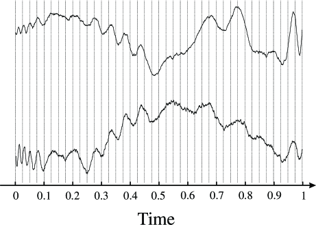
Figure 15: Two signals coupled by an unobserved phenomenon. The signals tend to change their intermediate trends synchronously, while their overall shapes are different. The striking similarity is observed at intervals $[0,0.1]$ and $[0.2,0.55]$. Note also the common peaks at $t=0.675,0.775,0.975$. See details in Sect. 5.3.1.

Figure 15 displays the trajectories of two processes $F_{i}(t),~{}i=1,2$ coupled by the common underlying phenomenon which — by and large — makes them change their intermediate-scale trends synchronically. The most striking similarity between $F_{i}(t)$ is observed at the intervals $[0,0.1]$ and $[0.2,0.55]$. Also we note the synchronous peaks around $t=0.675,0.775,0.975$ (more pronounced for $F_{1}(t)$.) At the same time, the coupling phenomenon is not a primary one in shaping the dynamics of $F_{i}(t)$, so their overall outlooks are still quite dissimilar. In such situations one is interested in detection and proper quantification of the observed non-linear coupling. The problem of such a quantification constitutes an important part of modern analysis of time series.

MTA suggests an effective way of solving this problem by comparing the trend structures of observed series at different scales. We decompose the observations $F_{i}(t)$ into trees $M_{i}$ and calculate the distance $\mu$ (17) between different levels of these decompositions. The reciprocal $\mu^{-1}$ of the distance between the signals $F_{i}(t)$ is plotted as the function of the decomposition levels $l_{i},~{}i=1,2$ in Fig. 16a.

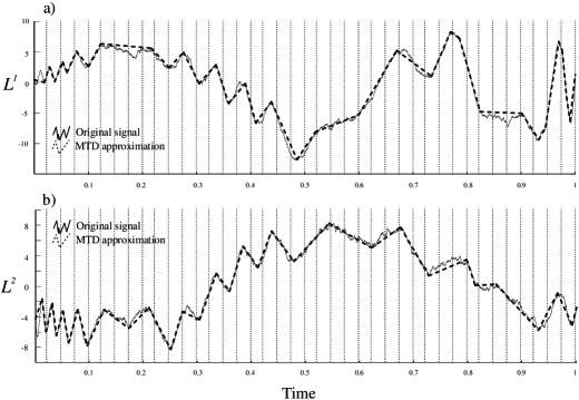
Figure 17: Piecewise linear approximations $L^{i},i=1,2$ of the signals $F_{i}(t)$ from Fig. 15 at the levels of maximal correlation $(l_{1}=15,l_{2}=14)$. These approximations depict the intermediate-scale variations responsible for the signals’ coupling.

The diagonal ridge indicates pairs of levels with similar trend structures. The prominent upwell observed at the medium scales — $15\leq l_{1}\leq 18,~{}14\leq l_{2}\leq 17$ — signals that this range is responsible for the observed coupling. The maximum $\mu^{-1}=4.6$ corresponds to the levels $l_{1}=15,~{}l_{2}=14$; we will refer to them as levels of maximal correlation (LMC). The piecewise linear approximations of $F_{i}(t)$ corresponding to the LMC are shown in Fig. 17. They clearly accentuate the observed coupling.

A typical shape of $\mu^{-1}$ for uncoupled time series is shown for comparison in Fig. 16b. The diagonal ridge is still observed, though it is more blurred. Existence of such a ridge is explained by the fact that partitions with a similar number of segments, even non-matching ones, are closer to each other in the sense of (17) than partitions with significantly different number of segments. Comparing Figs. 16a and b we conclude that the upwell observed in panel a is not a random one and is due to the correlation between the signals. A formal statistical test for establishing the significance of the observed peaks of $\mu$ can be easily constructed.

5.3.2 Quantification of detected correlation

As was shown in the previous section, MTA allows one to estimate non-linear correlations between signals; the value $\mu^{-1}$ may be considered as a measure of such correlation. Here we show how to evaluate the functional form of the coupling phenomenon responsible for the correlation detected.

To pose the problem formally, suppose that the observations $F_{i}(t),~{}i=1,2$ are formed by applying amplitude modulations $A_{i}(t)$ and adding non-linear trends $T_{i}(t)$ to the same base signal $X(t)$:

$$F_{i}(t)=A_{i}(t)\cdot X(t)+T_{i}(t)+\xi_{i}(t),~{}i=1,2.$$ (20)

Here $\xi_{i}(t)$ are measurement errors. In this model the correlation between signals $F_{i}(t)$ is due totally to the $X(t)$. The first problem is to reconstruct trends $T_{i}(t)$ and modulated signals $A_{i}(t)\cdot X(t)$ given the observations $F_{i}(t)$. Clearly, for reliable reconstruction one has to assume an appropriate rate of variation for the trends as well as a reasonably small noise-to-signal ratio. In practice, we assume that such conditions are satisfied if significant coupling has been detected by the correlation analysis of Sect. 5.3.1.

The idea of reconstruction is that the correlated parts $A_{i}\cdot X(t)$ should be described by the LMC of $M_{i}$ (see Sect. 5.3.1). Accordingly, the trends $T_{i}(t)$ should be described by the higher-scale (less detailed) levels.

As a model example we again use the series of Fig. 15; in fact, they are produced by the model (20) with

$$X(t) = \sin\left(400\pi t(t-0.5)(t-0.7)(t-1)\right);$$

$$T_{1}(t) = 5\sin\left(4\pi t^{3/2}\right);$$

$$~{}T_{2}(t) = -5\cos\left(2\pi t^{3/2}\right);$$

$$A_{1}(t) = \exp(2t);$$

$$~{}A_{2}(t) = 2\exp\left(-t/3\right).$$ (21)

The measurement errors $\xi_{i}(t)$ are modeled by independent Brownian walks so they also represent random drifts. The series $F_{i}(t)$ together with their components (5.3.2) are shown in Fig. 18.

The trends $T_{i}(t)+\xi_{i}(t)$ are estimated by the piecewise linear functions $\hat{T}_{i}$, formed by the parents of the vertices at the LMC, $l_{1}=15,~{}l_{2}=14$. In other words, each of the linear segments at the levels $l_{i}$ should be formed by a single non-trivial partition of one of the trends of $\hat{T}_{i}$. By single we mean that this is a one-time partition by the rules described in Sect. 2; by non-trivial — that each segment is divided into more than one subsegment. The modulated signals $A_{i}(t)\cdot X(t)$ are estimated then as $\widehat{A_{i}X_{i}}(t)=\left(F_{i}(t)-\hat{T}_{i}(t)\right),~{}i=1,2.$

The quality of these estimations is illustrated in Fig. 19 where we show real vs. estimated modulated signals $A_{i}X_{i}(t)$. The estimations are almost perfect at the intervals $[0,0.1]$ and $[0.2,0.55]$, (cf. Fig. 15 and its discussion in Sect. 5.3.1.) Generally, we catch well the oscillatory structure of the signals; that is their time-dependent frequencies and directions (upward vs. downward), while the amplitude estimation is less precise.

The estimations of Fig.19 can be further improved by means of various kernel smoothing techniques. MTA results can be used for optimization of the time-dependent kernel width.

With additional assumptions about the rate of variation for $A_{i}(t)$ one may pose the problem of reconstructing $X(t)$ given two, or more, modulated versions $A_{i}(t)\cdot X(t)$. Using the epochs assigned to the summands of (16) (say, $a_{i}$), one may analyze time-dependent correlations within $F_{i}(t)$. Clearly, the entire analysis can be repeated with the correlation (19) as a measure of trend similarity.

6 Discussion

The methods developed in this paper are based on the computational technique (see Sect. 2) for solving the linear interpolation problem for time series. This problem includes two principal difficulties. The first is a fundamental one: a tradeoff between the quality of a possible approximation and its detail. The second difficulty is purely computational: There are $(n-2)!/(n-1-k)!(k+1)!$ ways to construct a piecewise linear approximation with a given number $k$ of segments and $n$ observational epochs. Clearly, the search for the optimum over all possible approximations is unacceptable for operational use, and computationally effective algorithms are to be invented. Here we resolve the first difficulty by introducing the optimality criterion (3,4) of Sect. 2.2, and the second by replacing the original time series with its ”skeleton” that includes only the edge points defined in Sect. 2.3. The whole analysis is then done hierarchically, in a multiscale self-similar fashion. This contributes to computational efficiency as well as to the imprecision of the final result, since the errors made in the first steps of the decomposition may affect all the consecutive steps. It would therefore be interesting to study a) deviations of the MTA approximations from the optimal (in a squared deviation sense) piecewise linear approximations with the same number of segments, and b) the history of the first-step errors.

The procedure for edge point detection is introduced here (Sect. 2.3) in its simplest (not to say most naive) form and is subject to further improvement. Nevertheless, even in its present form, the MTA has the potential to be an effective tool for solving a wide specrtrum of applied problems, ranging from exploratory data analysis to studying hierarchical scaling for time series.

Recently, several techniques based on properties of local linear trends were proposed and studied. The Detrended Fluctuation Analysis (DFA) [7] was shown to be a powerful tool for multiscale analysis and interpretation of diverse medical and financial data. Contrary to our analysis, DFA uses a predefined interval partition scheme independent of the particular series at hand. It is oriented toward analysis of variations, rather than the trend structure itself. An alternative approach to the problem of detection of local linear trends is discussed in [13].

The problem considered in this paper naturally extends to higher dimensions. However, it is not clear how to apply the ideas developed here even to 2D and this issue deserves special attention. Interestingly, elegant theoretical results on rectifiable curves by P. Jones [14] are tightly related to detection of linear structures in point clouds. Various methods of multiscale geometric analysis based on Jones’ theory ([15] and references therein) use predefined (dyadic) partition schemes. It would be very important to find algorithms for fast linearization in point clouds.

It is worth mentioning that the self-affine analysis of Sect. 3 may be done equally effectively by a multitude of techniques, and MTA is by no means claimed to be the most efficient one. We include this section in order to demonstrate the diversity of possible applications based on the single MTA decomposition of a time series.

Acknowledgments. We are grateful to Robert Mehlman for valuable discussion and David Shatto for help in preparation of this paper. This work was supported by a Collaborative Activity Award for Studying Complex Systems from the 21st Century Science Initiative of the James S. McDonnell Foundation and INTAS 0748.

Appendix A Mandelbrot cascade measures

A Mandelbrot cascade measure $M(r_{i},m_{i})$, $i=1,\dots,n$ on the interval $[0,~{}1]$ is constructed as follows. At step 0 there is a unit mass distributed uniformly over the whole interval. At the first step we divide the interval $[0,~{}1]$ into $n$ subintervals of lengths $r_{i}$, $\sum_{i=1}^{n}r_{i}=1$ and assign to them masses $m_{i}$, $\sum_{i=1}^{n}m_{i}=1$. Within each interval the mass distribution is uniform. Next, we divide each subinterval $i$ into $n$ subsubintervals and assign to them uniform masses $m_{i}\cdot m_{j}$, $j=1,\dots,n$, and so on. Therefore, at the $k$th step the interval $[0,~{}1]$ is divided into $n^{k}$ subintervals, each carrying the uniform mass $m_{i_{1}}\cdot\dots\cdot m_{i_{k}}$, with $i_{k}$ taken from the set $1,\dots,n$ with possible repetitions.

Such measures were introduced first to model turbulent dissipation, and were studied by Mandelbrot [16].

Figure 12: Three levels of detail in MTA description of a time series. a) Topological. b) r-metric, based on the interval partition. c) e-metric, based on local linear fit of the series. See details in Sect. 4.

Figure 16: Correlation (reciprocal distance) $\mu$ (17) between two signals shown in Fig. 15 (panel a) and two independent Brownian walks (panel b).

Figure 18: Structure of the signals $F_{i}(t),i=1,2$ shown in Fig. 15. a),e) Original signals $F_{i}(t)$. b),f) Coupling parts $A_{i}(t)\cdot X(t)$. c),g) Non-linear deterministic trends. d),h) Random drifts.

Figure 19: Reconstruction (solid lines) of the coupling parts $A_{i}(t)\cdot X(t)$ (dashed lines). See Sect. 5.3.1 for discussion.

References

- [1] J. Sklansky and V. Gonzalez, Pattern Recognition 12, 327 (1980).
- [2] J. Roberge, Computer Vision, Graphics and Image Processing 29, 168 (1985).
- [3] B. K. Natarajan, SIAM Conference on Geometric Design. (1991).
- [4] R. Badii and A. Politi, Complexity: Hierarchical Structures and Scaling in Physics, (Cambridge University Press, 1997), p. 318.
- [5] B. Mandelbrot, Gaussian Self-Affinity and Fractals, (Springer Verlag, 2001), p. 664.
- [6] D. L. Turcotte, Fractals and Chaos in Geology and Geophysics., 2nd ed. (Cambridge University Press, 1997), p. 398.
- [7] C.-K. Peng, S. Havlin, H. E. Stanley, A. L. Goldberger, Chaos, 5, 82 (1995).
- [8] R. E. Horton, Geol. Soc. Am. Bull., 56, 275 (1945).
- [9] A. N. Strahler, Trans. Am. Geophys. Un., 38, 913 (1957).
- [10] W. I. Newman, D. L. Turcotte, and A. M. Gabrielov, Fractals, 5, 603 (1997).
- [11] A. Gabrielov, W. I. Newman, and D. L. Turcotte, Phys. Rev. E, 60, 5293 (1990).
- [12] Z. Toroczkai, Phys. Rev. E, 65, 016130 (2001).
- [13] J. T.-Y. Cheung and G. Stephanopoulos, Computer Chem. Eng., 14, 495 (1990).
- [14] P. W. Jones, Invent. Math., 102, 1 (1990).
- [15] G. Lerman, To appear in Communications on Pure and Applied Math. (2003).
- [16] B. Mandelbrot, J. Fluid Mech., 62, 331 (1974).