Vortex lines of the electromagnetic field

Abstract

Relativistic definition of the phase of the electromagnetic field, involving two Lorentz invariants, based on the Riemann-Silberstein vector is adopted to extend our previous study [I. Bialynicki-Birula, Z. Bialynicka-Birula and C. Śliwa, Phys. Rev. A 61, 032110 (2000)] of the motion of vortex lines embedded in the solutions of wave equations from Schrödinger wave mechanics to Maxwell theory. It is shown that time evolution of vortex lines has universal features; in Maxwell theory it is very similar to that in Schrödinger wave mechanics. Connection with some early work on geometrodynamics is established. Simple examples of solutions of Maxwell equations with embedded vortex lines are given. Vortex lines in Laguerre-Gaussian beams are treated in some detail.

I Introduction

The physical significance of the singularities of the phase of quantum mechanical wave functions has been recognized by Dirac in his work on magnetic monopoles dirac . The hydrodynamic formulation of the Schrödinger theory discovered by Madelung madelung provided a vivid interpretation of the lines in space where the phase is singular. These are simply the vortex lines in the flow of the probability fluid. The velocity field ${\bm{v}({\bm{r}},t)}$ of this fluid, defined in terms of the probability current ${\bm{j}}$, is equal to the gradient of the phase $S$ of the wave function $\psi=R\exp(iS/\hbar)$,

$${\bm{v}}=\frac{{\bm{j}}}{\rho}=\frac{\hbar}{2mi}\frac{\psi^{*}{\bm{\nabla}}\psi-{\bm{\nabla}}\psi^{*}\psi}{|\psi|^{2}}=\frac{{\bm{\nabla}}S}{m}.$$ (1)

Therefore, the flow is strictly irrotational in the bulk; vorticity may live only on the lines of singularities of the phase. Regular wave functions may have a singular phase only where the wave function vanishes, i.e. where $\Re\psi=0$ and $\Im\psi=0$. These two equations define two surfaces in space whose intersection determines the position of vortex lines. However, the vanishing of the wave function is the necessary but not the sufficient condition for the existence of vortex lines. They exist only if the circulation around the line where the wave function vanishes is different from zero. The univaluedness of the wave function requires the quantization of the circulation

$$\oint{\bm{d}l}\!\cdot\!{\bm{v}}=2\pi n\hbar/m.$$ (2)

The importance of this condition in the hydrodynamic formulation of wave mechanics has been elucidated for the first time by Takabayasi takabayasi . If Eq. (2) holds for every closed contour, we may recover the phase $S$ (modulo $2\pi\hbar$) from ${\bm{v}}$ up to a global, constant phase with the help of the formula

$$S({\bm{r}})=m\int_{{\bm{r}}_{0}}^{{\bm{r}}}{\bm{d}l}\!\cdot\!{\bm{v}}.$$ (3)

Early studies of vortex lines were restricted to wave mechanics but Nye and Berry nye_berry ; berry ; nye_book ; berrySPIE have shown that phase singularities or wavefront dislocations play an important role not only in wave mechanics but in all wave theories. A general review of phase singularities in wave fields has been recently given by Dennis dennis ; dennis1 . There is a substantial overlap of concepts (but not of the results) between our work and the works of Berry, Nye and Dennis. While they concentrate mostly on the stationary vortex lines that are found in monochromatic fields, we emphasize the time evolution.

More recently, the study of phase singularities and vortices in optics has evolved into a separate area of research, both theoretical and experimental, called singular optics. A recent review of this field is given in Ref. sos_vas .

In order to find a natural generalization of Eq. (1), we need a replacement for the wave function $\psi$ in electromagnetism. A suitable object appears in the complex form of Maxwell equations known already to Riemann riem and investigated more closely by Silberstein silber at the beginning of the last century. In this formulation the electric and magnetic field vectors are replaced by a single complex vector ${\bm{F}}$ that we proposed to call the Riemann-Silberstein (RS) vector ibbapp ; ibbwf

$${\bm{F}}=({\bm{E}}+i{\bm{B}})/\sqrt{2}.$$ (4)

Maxwell equations in free space written in terms of ${\bm{F}}$ read ($c=1$)

$$i\partial_{t}{\bm{F}} = \nabla\times{\bm{F}},$$ (5a)

$$\nabla\cdot{\bm{F}} = 0.$$ (5b)

The analogy between Eq. (5a) and the Schrödinger wave equation is so close that one is lead to treat ${\bm{F}}$ as the photon wave function ibbwf and apply similar methods to analyze the vortex lines and their motion as we have done in Refs. bbs ; bmrs in nonrelativistic wave mechanics. There is, however, an important difference that requires an extension of our previous methods: the RS vector has three components instead of one. Thus, there are three independent phases $\varphi_{1}$, $\varphi_{2}$, $\varphi_{3}$ — one for each component and it is not clear which combination of these phases should be treated as an overall phase of the electromagnetic field.

In the case of the the Schrödinger wave function, the information about the phase $S$ of the wave function is stored in the velocity field ${\bm{v}}={\bm{\nabla}}S/m$. Hence, one may try to find the proper definition of the phase of the electromagnetic field by introducing first the counterpart of Eq. (1) and then use the velocity field to reconstruct the phase. The natural generalization of the definition (1) is (in dimensionless form)

$${\bm{v}}=\frac{1}{2i}\frac{\sum_{k}\left(F_{k}^{*}{\bm{\nabla}}F_{k}-({\bm{\nabla}}F_{k}^{*})F_{k}\right)}{\sum_{k}F_{k}^{*}F_{k}}.$$ (6)

However, as has been noticed already by Takabayasi in his study of the hydrodynamic formulation of wave mechanics of spinning particles takabayasi1 , this generalization does not work. For a multicomponent field the velocity defined in this way cannot be used to reconstruct the phase because, in general, ${\bm{\nabla}}\times{\bm{v}}$ does not vanish. Even though one can still give a hydrodynamic interpretation of Maxwell theory based on the formula (1), the simplicity of the scalar case is completely lost ibb2 .

In the present paper, the phase of the electromagnetic field and the vortex lines associated with this phase are defined in terms of the square of the Riemann-Silberstein vector. Since ${\bm{F}}^{2}$ is a sum of two electromagnetic invariants, the structure of phase singularities associated with ${\bm{F}}^{2}$ is relativistically invariant. This definition of the phase turns out to be equivalent (provided ${\bf F}$ obeys Maxwell equations) to the one used in the classic papers on geometrodynamics rainich ; mw ; witten .

Despite the fact that ${\bm{F}}^{2}$ does not obey any simple wave equation, the time evolution of the vortices exhibits all the typical features found before by us for the Schrödinger equation. During the time evolution governed by Maxwell equations vortex lines are created and annihilated at a point or in pairs and undergo vortex reconnections.

II Geometrodynamics and the phase of the electromagnetic field

In nonrelativistic wave mechanics the phase of the wave function can be obtained from its modulus provided we also assume that the wave function obeys the Schrödinger equation. As a matter of fact it was shown by E. Feenberg kemble that to determine the phase from the modulus it is sufficient that the wave function obeys some wave equation that leads to conservation of the probability, i.e. to continuity equation. A similar reasoning applied to the electromagnetic field also enables one to determine the (properly defined) phase of this field. This discovery has been made by Rainich rainich in connection with the problem of the reconstruction of the electromagnetic field from purely geometric quantities in general relativity. Independently, although much later, this problem was solved by Wheeler and coworkers mw ; witten ; mtw ; pr in the context of geometrodynamics.

Very briefly, the reconstruction of the electromagnetic field from geometry may be described as follows. The Einstein equations

$$R_{\mu\nu}-g_{\mu\nu}R/2=\kappa T_{\mu\nu}$$ (7)

enable one to determine the energy-momentum tensor $T_{\mu\nu}$ of the electromagnetic field from the Einstein tensor $R_{\mu\nu}-g_{\mu\nu}R/2$ that is made of the metric tensor and its derivatives. However, the knowledge of the energy-momentum tensor alone is not sufficient to determine completely the electromagnetic field. This is best seen from the formulas for the components of this tensor expressed in terms of the RS vector:

$$T_{00} = {\bm{F}}^{*}\cdot{\bm{F}},$$ (8a)

$$T_{0i} = \epsilon_{ijk}F^{*}_{j}F_{k}/i,$$ (8b)

$$T_{ij} = -F^{*}_{i}F_{j}-F^{*}_{j}F_{i}+\delta_{ij}{\bm{F}}^{*}\!\cdot\!{\bm{F}}.$$ (8c)

All components of the energy-momentum tensor are invariant under the common change of the phase of all three components of the RS vector — the duality transformation

$${\bm{E}}^{\prime}={\bm{E}}\cos\varphi-{\bm{B}}\sin\varphi,$$ (9a)

$${\bm{B}}^{\prime}={\bm{E}}\sin\varphi+{\bm{B}}\cos\varphi.$$ (9b)

Therefore, the overall phase cannot be determined from the energy-momentum tensor. Note, that in contrast to the situation in quantum mechanics, even the global, constant phase of ${\bm{F}}$ has a direct physical meaning. It controls the relative contribution to the energy-momentum tensor from the electric and the magnetic parts. The duality rotations (9) with a constant value of $\varphi$ leave the free Maxwell equations unchanged. However, a phase varying in space and/or time would modify the Maxwell equations. That is the reason why the Rainich construction works. Namely, he has shown that if one assumes that the electromagnetic field obeys Maxwell equations, the phase of the field may be extracted from $T_{\mu\nu}$. For this purpose he introduced the following four-vector built from the components of the energy-momentum tensor and its derivatives

$$w^{\mu}=-\frac{\epsilon^{\mu\nu\lambda\rho}T_{\nu\kappa}\partial_{\lambda}T^{\kappa}_{\;\;\rho}}{T_{\sigma}^{\;\tau}T_{\tau}^{\;\sigma}}$$ (10)

and used the line integral of $w^{\mu}$ to reconstruct the phase.

Our proposal, how to define the phase of the electromagnetic field is much simpler and yet it turns out to be completely equivalent to the definition given by Rainich. We shall define the phase of the electromagnetic field $\varphi(x)$ as half of the phase of the square of the RS vector

$${\bm{F}}^{2}(x)=e^{2i\varphi(x)}|{\bm{F}}^{2}(x)|.$$ (11)

In full analogy with Eq. (1) of nonrelativistic wave mechanics, we define a “velocity” four-vector $u^{\mu}$ as

$$u_{\mu}=\frac{({\bm{F}}^{2})^{*}\partial_{\mu}{\bm{F}}^{2}-{\bm{F}}^{2}\partial_{\mu}({\bm{F}}^{2})^{*}}{4i|{\bm{F}}^{2}|^{2}}=\partial_{\mu}\varphi(x).$$ (12)

Since ${\bm{F}}^{2}$ is a complex sum of two electromagnetic invariants

$${\bm{F}}^{2}={\cal S}+i{\cal P}=\frac{1}{2}({\bm{E}}^{2}-{\bm{B}}^{2})+i{\bm{E}}\!\cdot\!{\bm{B}},$$ (13)

$u_{\mu}$ is a true relativistic four-vector

$$u_{\mu}=\frac{{\cal S}\partial_{\mu}{\cal P}-{\cal P}\partial_{\mu}{\cal S}}{2({\cal S}^{2}+{\cal P}^{2})}.$$ (14)

This vector has the same denominator (up to a factor of 2 that scales both the numerator and the denominator) as the vector $w^{\mu}$ defined by Eq. (10) since $T_{\sigma}^{\;\tau}T_{\tau}^{\;\sigma}=4({\cal S}^{2}+{\cal P}^{2})$. However, in general, the numerators of vectors $w_{\mu}$ and $u_{\mu}$ are different. They do become equal when the electromagnetic field obeys the Maxwell equations. The proof is straightforward but rather tedious and will not be presented here.

In our formulation, the square of the RS vector plays the role of the wave function $\psi$. Vortex lines are to be found at the intersection of the ${\cal S}=0$ and ${\cal P}=0$ surfaces. As in the case of the Schrödinger wave function, at all points where ${\bm{F}}^{2}$ does not vanish, the vector $u_{\mu}$ is by construction a pure gradient

$$u_{\mu}(x)=\partial_{\mu}\varphi(x).$$ (15)

Therefore, one may recover the phase of ${\bm{F}}$ by the following line integral

$$\varphi(x)=\int_{\bm{x}_{0}}^{\bm{x}}\!d{\xi}^{\mu}u_{\mu}({\xi}).$$ (16)

Since the RS vector is univalued, the phases obtained by choosing different paths connecting the points $x$ and $x_{0}$ may differ only by a multiple of $2\pi$. In other words, the vorticity associated with $u_{\mu}$ (or with $w_{\mu}$ in the Rainich construction) must be quantized

$$\oint\!d{\xi}^{\mu}u_{\mu}({\xi})=2\pi n.$$ (17)

The phase defined by Eq. (16) is determined up to a global phase $\varphi_{0}$: the value of $\varphi(x)$ at the lower limit $x_{0}$ of the integral. The value of $\varphi_{0}$ cannot be obtained from the energy-momentum tensor.

Under duality rotations (9) when $\varphi$ varies from 0 to $2\pi$, the vector ${\bm{E}}^{\prime}$ at each spacetime point draws an ellipse in the ${\bm{E}}-{\bm{B}}$ plane. The same ellipse is drawn by the vector ${\bm{B}}^{\prime}$. These ellipses become circles on each vortex line since then the vectors ${\bm{E}}$ and ${\bm{B}}$ are orthogonal and of equal length. This property lead Berry and Dennis dennis to name the vortex lines associated with the square of a complex vector field the C (circle) lines in their general classification scheme of phase singularities.

The denominator in Eq. (14) may be also expressed in the form

$${\cal S}^{2}+{\cal P}^{2}=\left(\frac{{\bm{E}}^{2}+{\bm{B}}^{2}}{2}\right)^{2}-({\bm{E}}\times{\bm{B}})^{2}.$$ (18)

Therefore, the vanishing of ${\cal S}^{2}+{\cal P}^{2}$ at a point also means that the electromagnetic field at this point is pure radiation: the energy density and the Poynting vector form a null four-vector. One may say that on vortex lines the energy of the electromagnetic field moves locally with the speed of light. We would like to emphasize that the velocity of the energy flow of the electromagnetic field is not correlated with the vector $u_{\mu}$. Even the geometric properties of the Poynting vector and the space part of $u_{\mu}$ are different. Since ${\cal S}$ is a scalar and ${\cal P}$ is a pseudoscalar, the vector $u_{\mu}$ is a pseudovector. In the simplest case of a constant electromagnetic field the Poynting vector is ${\bm{E}}\times{\bm{B}}$, while the vector $u_{\mu}$ vanishes identically. There does not seem to exist a physical quantity whose flow can be identified with $u_{\mu}$. In this respect the situation is quite different from nonrelativistic wave mechanics where the gradient of the phase determines the velocity of the probability flow.

III Simple examples of vortex lines

The analogy between the phase of wave function and the phase of the electromagnetic field is not exact. Unlike the Schrödinger wave function, the electromagnetic field does not have to vanish identically along the lines where the phase is singular. It is only necessary that the field is null i.e. the two invariants ${\cal S}$ and ${\cal P}$ vanish. Still, we believe that the lines along which the field is null deserve the name of vortex lines.

The time evolution of the vortex lines embedded in the solutions of the Maxwell equations is quite similar to the evolution of such lines embedded in the solutions of the Schrödinger equation. The simplest examples of solutions with vortex lines can again be found among the polynomial functions. Such functions may be viewed as long wavelength expansions and were found to be very useful in the study of vortex solutions of the Schrödinger equation bbs ; bmrs and the Helmholtz equation nye_berry ; berry_dennis . Alternatively, these polynomial solutions may be viewed as local approximations to the full solution, valid close to the vortex lines under study. In this case one may imagine that in the exact solution the polynomial is multiplied by some slowly varying envelope that makes the full solution localized. We shall give at the end of this Section an example of such a solution.

As an illustration of a typical behavior of electromagnetic vortex lines, we present very simple examples of the electromagnetic field. The following four fields satisfy the Maxwell equations and possess the vortex structures very similar to those found in Schrödinger wave mechanics bbs ; bmrs

$${\bm{F}}^{(a)} = \{y+it,z-a+i(a+t),x+it\},$$ (19a)

$${\bm{F}}^{(b)} = \{y+t,a-i(z+a+t),x+it\},$$ (19b)

$${\bm{F}}^{(c)} = \{2x+y-a+i(z+y+t),z-y+t+i(y-a),-t+it\},$$ (19c)

$${\bm{F}}^{(d)} = \{z^{2}+t^{2}-iat,a^{2}-i(2zt+a^{2}+ax),a(y-t)\},$$ (19d)

where $a$ is a parameter that sets the scale for the vortex configuration. In the first three cases the electromagnetic fields are linear functions of the coordinates and in the last case the field is quadratic. In the first case, the two invariants are

$${\cal S} = x^{2}+y^{2}+(z-a)^{2}-a^{2}-2at-3t^{2},$$ (20a)

$${\cal P} = 2az+2t(x+y+z-a)-2a^{2}.$$ (20b)

The equations ${\cal S}=0$ and ${\cal P}=0$ describe a sphere centered at the point $(0,0,a)$ with the time dependent radius $\sqrt{a^{2}+2at+3t^{2}}$ and a moving plane, respectively. The intersection of these two surfaces is a moving ring shown in Fig. 1. The radius of the sphere decreases for negative values of $t$ until $t=-a/3$ and then starts increasing. The rate of change of the radius exceeds (by a factor of $\sqrt{3}$) the speed of light showing once again that various characteristic features of relativistic fields (like their zeros or maxima) may travel with superluminal speeds without violating causality. In this simple example, no change of the topology of vortex line takes place. However, in the three remaining cases the topology changes according to the same universal patterns as those found in Schrödinger wave mechanics. This universal behaviour of vortex lines is reminiscent of the catastrophe theory nye1 ; berry1 .

The graphical representation of the motion of the vortex lines in all four cases is straightforward since the equations ${\cal S}=0$ and ${\cal P}=0$ can be solved analytically giving $x$ and $y$ for each value of $t$ as parametric functions of $z$. In each case there are two branches that differ by the sign of the square root.

$$x(z,t) = \left((a-z)(a+t)\pm\sqrt{a^{2}+2at+3t^{2}}\sqrt{2t^{2}-(a-z)^{2}}\right)/(2t),$$

$$y(z,t) = \left((a+t)(a-z)\mp\sqrt{a^{2}+2at+3t^{2}}\sqrt{2t^{2}-(a-z)^{2}}\right)/(2t),$$ (21a)

$$x(z,t) = a(a+z)/t-a,$$

$$y(z,t) = -t\pm\sqrt{t^{2}-a^{2}}\sqrt{a^{2}-2at+2t^{2}+2az-2zt+z^{2}}/t,$$ (21b)

$$x(z,t) = t+\left(t^{2}\pm\sqrt{t^{4}-8t^{2}(z-a)z-16(z-a)^{2}z^{2}}\right)/(4(z-a)),$$

$$y(z,t) = (a-z)/2+\left(t^{2}\mp\sqrt{t^{4}-8\,t^{2}(z-a)z-16(z-a)^{2}z^{2}}\right)/(8z),$$ (21c)

$$x(z,t) = t\pm\sqrt{t^{2}-a^{2}}\sqrt{a^{4}+(t^{2}+z^{2})^{2}}/a^{2},$$

$$y(z,t) = -a-\left(t^{3}+zt(2a+z)\right)/a^{2}.$$ (21d)

The plots of the functions (b) and (d) show vortex creations and annihilations (Fig. 2 and Fig. 4) and for the functions (c) one obtains vortex reconnections (Fig. 3). Vortex annihilations occur at $t=-a$ and vortex creations occur at $t=a$. Note that according to the formulas (21b) and (21d), at these moments the vortex velocity $(dx/dt,dy/dt)$ becomes infinite.

It is also possible to construct localized, finite energy solutions of Maxwell equation with vortices. We shall give just one simple example of such a solution constructed from the following localized solution of the wave equation

$${\bm{Z}}({\bf r},t)=\{y,x,-t-i\tau\}((t+i\tau)^{2}-{\bf r}^{2})^{-2}.$$ (22)

With each vector solution of the wave equation one may associate a solution of Maxwell equations treating the solution of the wave equation as a complex counterpart of the Hertz potential. Namely, one may check the RS vector ${\bm{F}}({\bf r},t)$ constructed according to the following prescription bb

$${\bf F}({\bf r},t)=\nabla\times\left[i\partial_{t}{\bf Z}({\bf r},t)+\nabla\times{\bf Z}({\bf r},t)\right]$$ (23)

indeed satisfies the Maxwell equations. The square of the vector ${\bf F}$ has the form

$$32\frac{2(t^{2}+2x^{2}+2y^{2}-\tau^{2})+i(3x^{2}-3y^{2}+4t\tau)}{((t+i\tau)^{2}-{\bf r}^{2})^{6}}.$$ (24)

Since the numerator does not contain the variable $z$, the vortex lines embedded in this localized solution are straight lines parallel to the $z$ axis. Two pairs of such lines are created at $t=-\tau/3$ at the points $(\pm 2\tau/3,0)$ in the $xy$ plane. The four vortex lines move (Fig. 5) until they annihilate in pairs at $t=\tau/3$ at the points $(0,\pm 2\tau/3)$. The speed of each vortex line at the moment of creation and annihilation is infinite, showing very vividly that also for localized solutions of Maxwell equations the motion of vortex lines may be superluminal without any limitations. Arbitrarily high speed of vortex lines associated with solutions of the relativistic scalar wave equation has already been noted in Refs. nye_berry ; bbs .

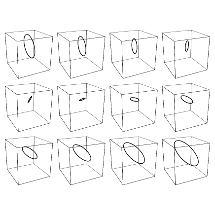
Figure 1: Time evolution of a vortex line in the form of a rotating and expanding ring. All figures in this paper were produced with the use of Mathematica wolfram .

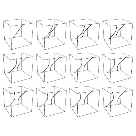
Figure 2: Time evolution of two vortex lines that at $t=a$ suddenly appear as a straight line and then separate and fly away. The same solution for negative times would show a reversed process: the convergence of two vortex line and their annihilation at $t=-a$.

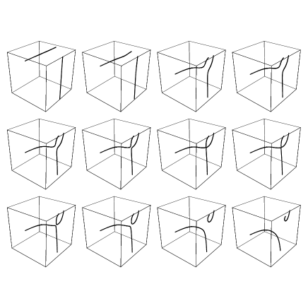
Figure 3: Time evolution of two vortex lines that at $t=0$ are mutually perpendicular and nonintersecting. At the time $t=a(\sqrt{2}-1)^{1/2}$ the vortex lines cross and undergo a reconnection.

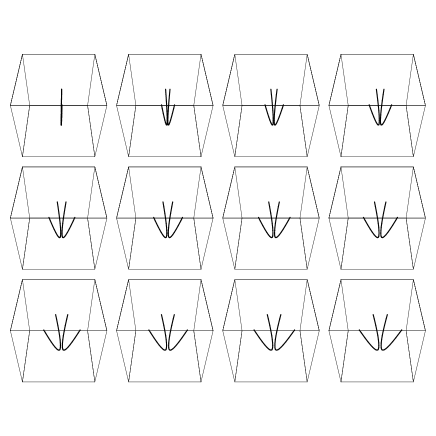
Figure 4: Time evolution of two vortex lines that at $t=a$ suddenly appear along a parabola in the $y=a$ plane (shown as a line in the first frame) that first opens up very fast into two symmetric wings that later slowly separate.

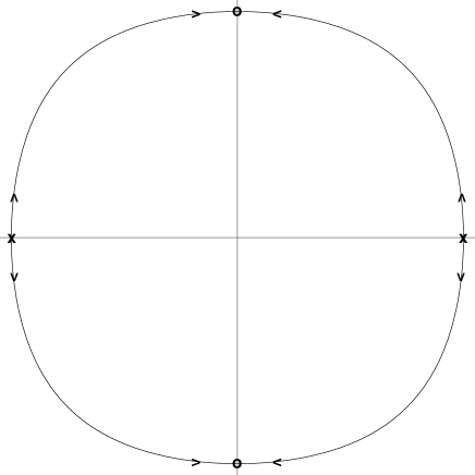
Figure 5: Time evolution in the $xy$ plane of two pairs of straight vortex lines parallel to the $z$ axis. The evolution is indicated by the arrows. Pairs of vortex lines are created at the points denoted by crosses and annihilated at the points denoted by circles.

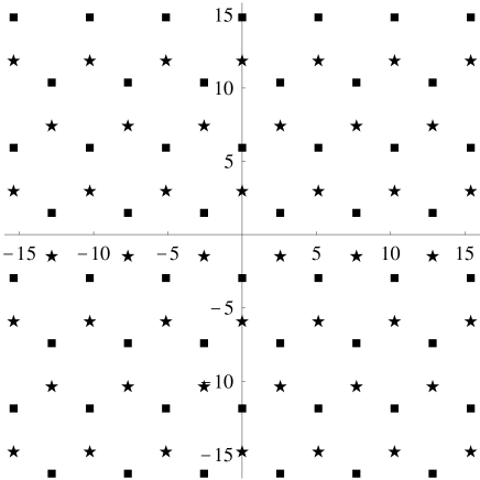
Figure 6: Positions of vortex lines in the $xy$ plane (measured in units of the inverse wave vector) for the three plane waves moving in orthogonal directions. Points marked with different symbols correspond to vortices with opposite circulation.

IV Vortex lines in superpositions of plane waves and in Gaussian beams

Solutions of Maxwell equations exhibiting vortex structures may also be obtained with the use of standard building blocks — the monochromatic plane waves. A single plane wave is described by a null field since both invariants vanish. Therefore, the velocity (14) vanishes — a single plane wave has no vortex structure. Also, the sum of two plane waves does not have any vortex structure; even though it has a nonvanishing velocity field. However, for three plane waves we may have various kinds of vortex structures. As an example, we choose three circularly polarized monochromatic waves of the same frequency, handedness, and amplitude, moving in three mutually orthogonal directions. The RS vector in this case (up to a constant amplitude) has the form

$${\bf F}({\bm{r}},t)=({\hat{\bm{m}}}+i{\hat{\bm{n}}})e^{-i(t-{\hat{\bm{l}}}\cdot{\bm{r}})}+({\hat{\bm{n}}}+i{\hat{\bm{l}}})e^{-i(t-{\hat{\bm{m}}}\cdot{\bm{r}})}+({\hat{\bm{l}}}+i{\hat{\bm{m}}})e^{-i(t-{\hat{\bm{n}}}\cdot{\bm{r}})},$$ (25)

where ${\hat{\bm{l}}},{\hat{\bm{m}}}$, and ${\hat{\bm{n}}}$ are three orthogonal unit vectors, the coordinates are measured in units of the inverse wave vector and time is measured in units of inverse angular frequency. The square of this vector vanishes at the points satisfying the equation

$$e^{i({\hat{\bm{l}}}+{\hat{\bm{m}}})\cdot{\bm{r}}}+e^{i({\hat{\bm{m}}}+{\hat{\bm{n}}})\cdot{\bm{r}}}+e^{i({\hat{\bm{n}}}+{\hat{\bm{l}}})\cdot{\bm{r}}}=0.$$ (26)

It is convenient to chose the coordinate system in such a way that the three basis vectors have the form

$${\hat{\bm{l}}}=\left(\begin{array}[]{c}\frac{1}{\sqrt{6}}\\ -\frac{1}{\sqrt{2}}\\ \frac{1}{\sqrt{3}}\end{array}\right),\;\;{\hat{\bm{m}}}=\left(\begin{array}[]{c}\frac{1}{\sqrt{6}}\\ \frac{1}{\sqrt{2}}\\ \frac{1}{\sqrt{3}}\end{array}\right),\;\;{\hat{\bm{n}}}=\left(\begin{array}[]{c}-\sqrt{\frac{2}{3}}\\ 0\\ \frac{1}{\sqrt{3}}\end{array}\right),$$ (36)

because then all the vortex lines are parallel to the $z$ axis. The position of the vortex lines in the $xy$ plane is determined by Eq. (26). For the choice (36) of unit vectors this equation has the form (apart from an overall phase-factor $\exp\left(i(\sqrt{2}\,x+2\,z)/\sqrt{3}\right)$)

$$1+e^{-i(\sqrt{3}x+y)/\sqrt{2}}+e^{-i(\sqrt{3}x-y)/\sqrt{2}}=0.$$ (37)

The solutions of this equation are

$$x^{\pm}_{mn}=\pi\sqrt{\frac{2}{3}}\;(m+n),\;\;y^{\pm}_{mn}=\pi\sqrt{2}\;(\pm\frac{2}{3}+m-n),\;\;$$ (38)

where $m$ and $n$ are arbitrary integers. The lattice of vortex lines is shown in Fig. 6. This example shows that vortex lines associated with the phase of the RS vector do not necessarily move; they can also be stationary.

When one of the polarizations of the three waves, say the last one in Eq. (25), is opposite, the position of vortex lines is determined by a time-dependent equation

$$e^{i({\hat{\bm{l}}}+{\hat{\bm{m}}})\cdot{\bm{r}}-2it}+e^{i({\hat{\bm{m}}}-{\hat{\bm{n}}})\cdot{\bm{r}}}+e^{i({\hat{\bm{l}}}-{\hat{\bm{n}}})\cdot{\bm{r}}}=0.$$ (39)

In this case it is convenient to choose the orthonormal unit vectors in the form

$${\hat{\bm{l}}}=\left(\begin{array}[]{c}\frac{1}{\sqrt{6}}\\ \frac{1}{\sqrt{2}}\\ \frac{1}{\sqrt{3}}\end{array}\right),\;\;{\hat{\bm{m}}}=\left(\begin{array}[]{c}\frac{1}{\sqrt{6}}\\ -\frac{1}{\sqrt{2}}\\ \frac{1}{\sqrt{3}}\end{array}\right),\;\;{\hat{\bm{n}}}=\left(\begin{array}[]{c}\sqrt{\frac{2}{3}}\\ 0\\ -\frac{1}{\sqrt{3}}\end{array}\right).$$ (49)

The position of vortex lines in the $xy$ plane is determined by the equation

$$1+e^{-i(\sqrt{3}x+y)/\sqrt{2}+2it}+e^{-i(\sqrt{3}x-y)/\sqrt{2}+2it}=0.$$ (50)

Thus, in this case the lattice of vortex lines is not stationary but it is moving as a whole with the speed of $\sqrt{8/3}c$ in the $x$ direction.

The most interesting case, of course, is a superposition not of a few but of a continuum of plane waves, forming a collimated beam. We shall concentrate on the Laguerre-Gaussian beams, in view of their applicability to realistic situations (cf., for example wright ). We use the representation of these beams in the vector theory as in Refs.absw ; allen0 ; allen ; sps but we combine the electric and the magnetic field vectors into the complex RS vector (4). This vector for Laguerre-Gaussian beams of circular polarization can be written in the form

$${\bm{F}}(x,y,z,t)=e^{-i(\omega t-kz)}\left(ku,iku,i(\partial_{x}u+i\partial_{y}u)\right).$$ (51)

The square of the this vector is equal to

$$({\bm{F}}(x,y,z,t))^{2}=-e^{-2i(\omega t-kz)}((\partial_{x}+i\partial_{y})u)^{2}.$$ (52)

Note, that the vector ${\bm{F}}$ given by Eq. (51) is not just the analytic signal but the full RS vector as defined by Eq. (4) whose real part is the electric field and the imaginary part is the magnetic induction. The slowly varying complex envelope function $u=u(x,y,z)$ is an arbitrary linear superposition of the functions $u_{nm}(\rho,\phi,z)$ defined as (we use the notation of Ref. sps )

$$u_{nm}(\rho,\phi,z)=C_{nm}\frac{w_{0}}{w(z)}\exp\left[-\tilde{\rho}^{2}\right]\exp\left[\!\frac{ik\rho^{2}z}{2(z^{2}+z_{R}^{2})}\right]\left(\sqrt{2}\,\tilde{\rho}\right)^{|m|}\!L^{|m|}_{n}(2\tilde{\rho}^{2})\,e^{im\phi}e^{-i(2n+|m|+1)\arctan(z/z_{R})},$$ (53)

where $C_{nm}$ is the normalization constant, $w(z)=w_{0}\sqrt{1+(z/z_{R})^{2}}$ is the $z$-dependent radius of the beam, $\tilde{\rho}$ is the radial coordinate divided by $w(z)$, $L^{m}_{n}$ is the generalized Laguerre polynomial, and $z_{R}=\pi w_{0}/\lambda$ is the Rayleigh length. The functions $u_{nm}$ describe the beam with the projection of the orbital angular momentum on the propagation axis defined by $m$. They may be written in the form

$$u_{nm}(\rho,\phi,z)=(x\pm iy)^{|m|}f_{nm}(\rho,z),$$ (54)

where the upper sign corresponds to the positive values of $m$. This leads to the following formula

$$(\partial_{x}+i\partial_{y})(x\pm iy)^{|m|}f_{nm}$$

$$=(x\pm iy)^{|m|\pm 1}\rho^{\mp 1}(\partial\!f_{nm}/\partial\rho+(1\mp 1)f_{nm}/\rho).$$ (55)

The velocity (12) can be obtained by differentiating the phase of the function $(\partial_{x}+i\partial_{y})u$ but the expression is quite cumbersome. However, it is clear from Eq. (IV) that the function $(\partial_{x}+i\partial_{y})u$ for positive and for negative values of $m$ carries $m+1$ units of angular momentum in the $z$ direction. Vortex lines defined in terms of the RS vector run along the $z$ axis and their vorticity has the strength $m+1$. At first, these results seem to be in disagreement with the detailed analysis of angular momentum of Laguerre-Gauss beams by Allen, Padget, and Babiker given in Ref. allen since they have shown that the additional unit of angular momentum is to be added to $m$ or subtracted from $m$ depending on the (right or left) polarization of the beam. However, we have broken this symmetry by considering the RS vector ${\bm{F}}$ and not its complex conjugate. This (arbitrary) choice has fixed the (positive) sign of the polarization. With this proviso, our definition of vortex lines in terms of the RS vector leads to the same results as the analysis of angular momentum. Each component $u_{nm}$ has only one vortex line associated with the total angular momentum. However, superpositions of several $u_{nm}$ components, depending on their composition, may have additional vortex lines.

The presence of vortex lines in Laguerre-Gaussian beams is due to the definite angular momentum in the direction of propagation. The same vortex lines appear also in electromagnetic multipole fields. In this case the RS vector can be written in the form zib

$${\bm{F}}(x,y,z,t)=e^{-i\omega t}(k+\nabla\times)j_{J}(kr)({\bm{r}}\times\nabla)Y_{JM}(\hat{\bm{r}}).$$ (56)

For the dipole field ($J=1,\;M=1$)

$$\left({\bm{F}}(x,y,z,t)\right)^{2}=e^{-2i\omega t}(x+iy)^{2}\frac{\left(3+4k^{2}r^{2}-2k^{4}r^{4}+(2k^{2}r^{2}-3)\cos(2kr)-6kr\sin(2kr)\right)}{2k^{6}r^{8}}.$$ (57)

Thus, the dipole field for $M=1$ exhibits one vortex line along the $z$-axis (the direction of the angular momentum quantization) with unit vorticity. Higher multipoles will exhibit vortex lines carrying more units of vorticity, depending on the value of the $z$ component of the angular momentum.

V Conclusions

The study presented in this paper fully unifies the description of vortex lines in electromagnetism and in Schrödinger wave mechanics. In both cases there is a single complex function of space and time whose phase generically has singularities along one-dimensional curves in three-dimensional space — the vortex lines. The velocity four-vector $u_{\mu}$ associated with the phase of the electromagnetic field plays the same role as the velocity ${\bm{v}}$ of the probability fluid in wave mechanics. The circulation around each vortex line is quantized in units of $2\pi$. There are two important differences. First, the gradient of the electromagnetic phase does not have any obvious dynamical interpretation. Second, the electromagnetic field does not vanish identically on vortex lines but only the two relativistic invariants vanish and the energy-momentum becomes locally a null four-vector.

Finally, we would like to mention that in principle one should be able to construct a hydrodynamic form of electrodynamics, analogous to the Madelung formulation of wave mechanics. The set of hydrodynamic variables for the electromagnetic field would comprise the components of the energy-momentum tensor (only five of them are independent, cf., for example ibb2 ) and the velocity vector $u_{\mu}$ that carries the information about the phase of the RS vector. The quantization condition (17) effectively reduces the information contained in $u_{\mu}$ to just one scalar function giving finally six independent functions. However, we have not found a simple set of equations for these hydrodynamic-like variables that would be equivalent to Maxwell theory.

- (1) P. A. M. Dirac, Proc. Roy. Soc. Lond. A 133, 60 (1931).
- (2) O. Madelung, Z. Phys. 40, 322 (1926).
- (3) T. Takabayasi, Prog. Theor. Phys. 8, 143 (1952); 9, 187 (1953).
- (4) J. F. Nye and M. V. Berry, Proc. Roy. Soc. Lond. A 336, 165 (1974).
- (5) M. V. Berry, in Les Houches Lecture Series XXXV, edited by R. Balian, M. Kléman and J.-P. Poirier (North-Holland, Amsterdam, 1981), p. 453.
- (6) J. F. Nye, Natural Focusing and Fine Structure of Light: Caustics and Wave Dislocations (Institute of Physics Publishing, Bristol, 1999).
- (7) M.V. Berry, in Singular Optics (Optical Vortices): Fundamentals and Applications, edited by M.S. Soskin and M.V. Vasnetsov, SPIE 4403, 1 (2001).
- (8) M. R. Dennis, Topological Singularities in Wave Fields, PhD Thesis, U. of Bristol, 2001.
- (9) M. R. Dennis, Opt. Comm. 213, 201 (2002).
- (10) M.S. Soskin and M.V. Vasnetsov, Progress in Optics, Vol. XLI, edited by E. Wolf (Elsevier, Amsterdam, 2001).
- (11) H. Weber, 1901, Die partiellen Differential-Gleichungen der mathematischen Physik nach Riemann’s Vorlesungen (Friedrich Vieweg und Sohn, Braunschweig) p. 348.
- (12) L. Silberstein, Ann. d. Phys. 22, 579 (1907); 24, 783 (1907).
- (13) I. Bialynicki-Birula, Acta Phys. Pol. A 86, 97 (1994).
- (14) The history of the Riemann-Silberstein vector and its connection with the photon wave function is described in a review paper: I. Bialynicki-Birula, in Progress in Optics, Vol. XXXVI, edited by E. Wolf (Elsevier, Amsterdam, 1996).
- (15) I. Bialynicki-Birula, Z. Bialynicka-Birula and C. Śliwa, Phys. Rev. A 61, 032110 (2000).
- (16) I. Bialynicki-Birula, T. Młoduchowski, T. Radozycki and C. Śliwa, Acta Phys. Pol. A 100 (Supplement), 29 (2001).
- (17) T. Takabayasi, Prog. Theor. Phys. 14, 283 (1955).
- (18) I. Bialynicki-Birula, in Nonlinear Dynamics, Chaotic and Complex Systems, edited by E. Infeld, R.Zelazny, and A.Galkowski (Cambridge University Press, Cambridge, 1997).
- (19) E. C. Kemble, The Fundamental Principles of Quantum Mechanics (Dover, New York, 1958), p. 71.
- (20) G. Y. Rainich, Trans. Am. Math. Soc. 27, 106 (1925).
- (21) C. W. Misner and J. A. Wheeler, Ann. Phys. (NY) 2, 525 (1957).
- (22) L. Witten, in Gravitation: An Introduction to Current Research, Ed. L. Witten (Wiley, New York, 1962).
- (23) C. W. Misner, K. Thorn and J. A. Wheeler, Gravitation (Freeman, San Francisco, 1973).
- (24) R. Penrose and W. Rindler, Spinors and Space-Time (Cambridge University Press, Cambridge, 1986), Vol. I, Sec. 5.3.
- (25) M. V. Berry and M. R. Dennis, J. Phys. A 34, 8877 (2001).
- (26) S. Wolfram, Mathematica (Cambridge University Press, Cambridge, 1999).
- (27) J. F. Nye, JOSA A 15, 1132 (1998).
- (28) M. V. Berry, J. Mod. Opt. 45, 1845 (1998).
- (29) I. Bialynicki-Birula, Phys. Rev. Lett. 80, 5247 (1998).
- (30) K.-P. Marzlin, W. Zhang and E. M. Wright, Phys. Rev. Lett. 79, 4728 (1997).
- (31) L. Allen, M. W. Beijersbergen, R. J. C. Spreeuw and J. P. Woerdman, Phys. Rev. A 45, 8185 (1992).
- (32) L. Allen, V. E. Lembessis and M. Babiker, Phys. Rev. A 53, R2937 (1996).
- (33) L. Allen, M. J. Padgett and M. Babiker, Progress in Optics, Vol. XXXIX, edited by E. Wolf (Elsevier, Amsterdam, 1999).
- (34) Y. Y. Schechner, R. Piestun and J. Shamir, Phys. Rev. E 54, R50 (1996).
- (35) I. Bialynicki-Birula and Z. Bialynicka-Birula, Quantum Electrodynamics (Pergamon, Oxford, 1975).