Large Scale Evolution of Premixed Flames

Abstract

The influence of the small scale “cellular” structure of premixed flames on their evolution at larger scales is investigated. A procedure of the space-time averaging of the flow variables over flame cells is introduced. It is proved that to the leading order in the flame front thickness, the form of dynamical equations for the averaged gas velocity and pressure, as well as of jump conditions for these quantities at the flame front, is the same as in the case of a zero-thickness flame propagating in an ideal fluid at constant velocity with respect to the fuel, equal to the adiabatic velocity of a plane flame times a factor describing increase of the flame front length due to the local front wrinkling. As an application, the large scale evolution of a flame in the gravitational field is investigated. A weakly nonlinear non-stationary equation for the averaged flame front position is derived. It is found that the leading nonlinear gravitational effects stabilize the flame propagating in the direction of the field. The resulting stationary flame configurations are determined analytically.

I introduction

Propagation of plane flames in gaseous mixtures is well known to be unstable. An efficient way of investigating this instability is to consider the flame front as a surface of discontinuity, expanding all quantities of interest in powers of $L_{\rm f}/\lambda,$ where $L_{\rm f}$ is the flame front thickness, and $\lambda$ characteristic length scale of a flame perturbation. The leading term of the perturbation growth rate expansion has the form

$$\sigma=c_{0}\frac{U_{\rm f}}{\lambda}$$ (1)

where $U_{\rm f}$ denotes an adiabatic velocity of a plane flame front with respect to the fuel, and $c_{0}=c_{0}(\theta)$ a function of the gas expansion coefficient $\theta$ defined as the ratio of the fuel density ($\rho_{\rm u}$) and the density of burnt matter ($\rho_{\rm b}$), $\theta=\rho_{\rm u}/\rho_{\rm b}>1.$ According to Refs. landau ; darrieus , $c_{0}(\theta)$ has positive values for all $\theta,$ implying an unconditional instability of zero-thickness flames, the Landau-Darrieus (LD) instability. In the next order in $L_{\rm f}/\lambda,$ account of the transport processes inside the flame front modifies Eq. (1) to

$$\sigma=c_{0}\frac{U_{\rm f}}{\lambda}\left(1-c_{1}\frac{L_{\rm f}}{\lambda}\right)\,,$$ (2)

where $c_{1}$ depends on $\theta$ as well as on the ratio of the heat and mass diffusivities (the Lewis number) markstein ; pelce ; matalon . The product $c_{1}L_{\rm f}\equiv\lambda_{\rm c},$ the so-called cut-off wavelength, is the short wavelength limit of unstable perturbations. By the order of magnitude, $\lambda_{\rm c}$ represents also the characteristic length of the so-called cellular structure of the flame front, which is formed eventually as a result of the nonlinear flame stabilization. For many flames of practical interest, $c_{1}=15-20.$ It is the fact that $L_{\rm f}$ is relatively small in comparison with $\lambda_{\rm c}$ which underlies the above point of view on flame dynamics.

Consider an arbitrary initially smooth front configuration. As a result of the rapid growth of the unstable flame perturbations with wavelengths $\sim\lambda_{\rm c},$ the flame front becomes corrugated within the time interval

$$\Delta t\sim\frac{\lambda_{\rm c}}{U_{\rm f}}\,.$$ (3)

Dynamics of the short wavelength modes are mainly determined by the transport processes inside the flame front, and are affected only slightly by the large scale flow. One can say that the small scale cellular structure of the flame front develops on the “background” of its smooth large scale configuration (see Fig. 1). It follows all developments of the background, Eq. (3) playing the role of the characteristic time of cell adaptation to the large scale front evolution.

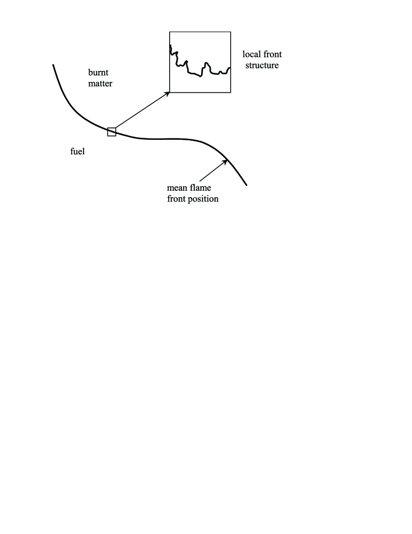
Figure 1: Schematic representation of the scale separation.

In practice, it is the large scale evolution of the flame front, rather than its exact local structure, which is often of the main concern. In this respect, an important question arises about the reverse influence of the flame cellular structure on the front evolution at scales much larger than $\lambda_{\rm c}.$ More precisely, one can state the problem as follows. Imagine that we have smeared the small scale rapid variations of all relevant quantities by averaging them over many flame cells. Then the question is what equations governing dynamics of the averages are.

In connection with the above statement of the problem it should be noted that the exact cellular structure of flames is actually unknown. This is because the process of cell formation is essentially nonlinear, in the sense that it cannot be treated perturbatively in principle, which is the main reason of lack of its theoretical description. Only in the case $\theta\to 1,$ which is practically irrelevant, can this structure be determined analytically henon ; siv1 ; sivclav ; kazakov1 ; kazakov2 . The question of principle, therefore, is to what extent the large scale dynamics of averages depend on the exact local flame structure in the regime of fully developed LD-instability.

The main purpose of the present paper is to show that to the leading order in the ratio of $\lambda_{\rm c}$ to the characteristic length of the problem ($L_{0}$), dynamics of the averaged quantities are actually independent of particularities of the local flame structure. The latter determines essentially only one parameter characterizing the large scale evolution – the effective normal velocity of the flame front.

Perhaps, it is worth to explain the essence of the problem in a little bit more detail. The above point of view on the flame propagation is based on the possibility to separate the local cellular dynamics from the large scale evolution of the background. This possibility is underlined by the following common property of the transport processes. From the mathematical point of view, all these processes are of higher differential order than those governing dynamics of an ideal fluid. Therefore, their relative role increases at smaller scales. In particular, in the limit $L_{\rm f}\to 0,$ cell formation is completely determined by the transport processes inside the flame front. On the contrary, the role of these processes at scales $L\gg L_{\rm f}$ is relatively small. It should be fully realized, however, that this reasoning is inherently linear. It tacitly assumes that if every quantity of interest, say $A,$ is represented as a sum of its averaged value $\langle A\rangle\equiv A_{0}$ and the small scale fluctuation $A_{1},$ then the dynamics of $A_{0}$’s can be determined solely in terms of $A_{0}$’s themselves. Because of the high nonlinearity of basic equations governing the flame propagation, this assumption is far from being self-evident. For instance, averaging of a cubic combination of $A$’s gives rise to a term $\langle A_{1}^{2}\rangle A_{0}$ comparable with $A_{0}^{3},$ since the small and large scale parts of the flow variables are generally of the same order of magnitude. Clearly, equations for $A_{0}$’s involving such terms would not be of great value, since the local flame dynamics, and therefore, the coefficients $\langle A_{1}^{2}\rangle,$ are unknown. The main result of the present work is the proof that such terms actually do not arise in the leading order with respect to $\lambda_{\rm c}/L_{0}.$ One can say that the governing equations for the quantities $A_{0}$ and $A_{1}$ decouple from each other. The proof consists of two parts corresponding to decoupling of the flow equations in the bulk, and decoupling of the jump conditions at the flame front, given in Secs. II.2 and II.3, respectively. As an application of this result, the problem of nonlinear front stabilization in a gravitational field will be considered in Sec. III. The results obtained are discussed in Sec. IV.

II The decoupling theorem

II.1 The averaging procedure

Let us begin with the precise formulation of the averaging procedure. Denote $L_{0}$ the characteristic length of the problem in question. For instance, $L_{0}$ can be the tube width, in the case of a flame propagating in a tube, or be related to an external field acting on the system. In practice, this length largely exceeds the flame cell size,

$$L_{0}\ggg\lambda_{\rm c}\,.$$

Assuming this, let us choose a length $L$ satisfying

$$\lambda_{\rm c}\ll L\ll L_{0}\,.$$

Analogously, denoting the characteristic time interval by $T_{0},$ and noting that

$$T_{0}\sim\frac{L_{0}}{U_{\rm f}}\,,$$

we can choose $T\sim L/U_{\rm f}$ such that

$$\frac{\lambda_{\rm c}}{U_{\rm f}}\ll T\ll T_{0}\,.$$

Given a function $A(\bm{x},t),$ we define its space-time average over $\{\bm{x},t:\bm{x}\in(\bm{x}_{0},\bm{x}_{0}+\Delta\bm{x}),$ $\Delta x_{i}=L,$ $~{}t\in(t_{0},t_{0}+T)\}$

$$\langle A\rangle=\frac{1}{L^{3}T}\int\limits_{T}dt\int\limits_{V}d^{3}\bm{x}~{}A(\bm{x},t)\equiv A_{0}(\bm{x}_{0},t_{0})\,.$$ (4)

By the definition, $\langle A\rangle$ varies noticeably over space distances $\|\Delta\bm{x}_{0}\|\sim L_{0},$ and time intervals $\Delta t_{0}\sim T_{0}.$ The function $A$ thus turns out to be decomposed into two parts corresponding to the two scales, $L_{0}$ and $\lambda_{\rm c}:$

$$A=A_{0}+A_{1},\qquad\langle A_{1}\rangle=0.$$

As was mentioned in the Introduction, flame dynamics can be analyzed in the framework of the power expansion with respect to the small ratio $L_{\rm f}/L_{0}\equiv\varepsilon$ (or equivalently, with respect to $\lambda_{\rm c}/L_{0},$ since $\lambda_{\rm c}=O(L_{\rm f})$). Thus, we write $A_{0}$ and $A_{1}$ as follows

$$A_{0}=A_{0}^{(0)}+\varepsilon A_{0}^{(1)}+\cdot\cdot\cdot\,,\quad A_{1}=A_{1}^{(0)}+\varepsilon A_{1}^{(1)}+\cdot\cdot\cdot\,,$$

dots denoting terms of higher order in $\varepsilon.$ In this notation, the large scale flame dynamics in zero order approximation with respect to $\varepsilon$ are described by the quantities $A_{0}^{(0)}.$ Our main purpose below will be to investigate coupling between $A_{0}^{(0)}$ and $A_{1}^{(0)},$ $A_{1}^{(1)},$ etc., and to obtain effective equations governing dynamics of $A_{0}^{(0)}.$ Accordingly, all quantities will be measured in units relevant to the large scale dynamics. Namely, space coordinates $\bm{x}$ and time $t$ are assumed to be normalized on $L_{0}$ and $L_{0}/U_{\rm f},$ respectively. Furthermore, $U_{\rm f}$ will be taken as the unit of gas velocity $\bm{v},$ while $\rho_{\rm u}U_{\rm f}^{2}$ as the unit of gas pressure $p\,.$ For future reference, let us write down their expansions explicitly

$$\bm{v}=\bm{v}_{0}+\bm{v}_{1}\,,\quad p=p_{0}+p_{1}\,,$$ (5)

$$\bm{v}_{0}=\bm{v}_{0}^{(0)}+\varepsilon\bm{v}_{0}^{(1)}+\cdot\cdot\cdot\,,\quad\bm{v}_{1}=\bm{v}_{1}^{(0)}+\varepsilon\bm{v}_{1}^{(1)}+\cdot\cdot\cdot\,,$$ (6)

$$p_{0}=p_{0}^{(0)}+\varepsilon p_{0}^{(1)}+\cdot\cdot\cdot\,,\quad p_{1}=p_{1}^{(0)}+\varepsilon p_{1}^{(1)}+\cdot\cdot\cdot\,.$$ (7)

Within our choice of units, we have the following estimates

$$\bm{v}_{0} = O(1),\quad\bm{v}_{1}=O(1),\quad p_{0}=O(1),\quad p_{1}=O(1),$$ (8)

$$\frac{\partial v_{0i}}{\partial x_{k}} = O(1),\quad\frac{\partial v_{0i}}{\partial t}=O(1),\quad\frac{\partial p_{0}}{\partial x_{k}}=O(1),$$ (9)

$$\frac{\partial v_{1i}}{\partial x_{k}} = O\left(\frac{1}{\varepsilon}\right),\quad\frac{\partial v_{1i}}{\partial t}=O\left(\frac{1}{\varepsilon}\right),\quad\frac{\partial p_{1}}{\partial x_{k}}=O\left(\frac{1}{\varepsilon}\right),$$ (10)

$$\quad\frac{\partial^{2}v_{0i}}{\partial x_{k}\partial x_{l}} = O(1)\,,\quad\frac{\partial^{2}v_{1i}}{\partial x_{k}\partial x_{l}}=O\left(\frac{1}{\varepsilon^{2}}\right)\,,\quad i,k,l=1,2,3.$$ (11)

Let us now proceed to the examination of flame dynamics in terms of $\bm{v}_{0,1}^{(0,1)},p_{0,1}^{(0,1)}.$

The main result concerning the large scale flame dynamics which will be proved below can be expressed in the form of the following

Decoupling theorem: The large scale dynamics of a flame are unaffected by its local cellular structure up to a rescaling. More precisely, the form of dynamical equations for $\bm{v}_{0}^{(0)},$ $p_{0}^{(0)},$ as well as of jump conditions for these quantities at the flame front, is the same as in the case of zero-thickness flame propagating in an ideal fluid at constant speed $\mathfrak{U}~{}U_{\rm f}$ with respect to the fuel, the number $\mathfrak{U}>1$ describing the flame front length increase due to the local front wrinkling.

The proof consists of two parts corresponding to decoupling of the flow equations in the bulk, and decoupling of the jump conditions at the flame front, presented in Secs. II.2 and II.3, respectively.

II.2 Decoupling of dynamical equations

For definiteness, we will assume in what follows that external field acting on the system is the gravitational field, denoting its strength by $\bm{g}.$ Accordingly, $L_{0}$ will be identified with the characteristic length associated with this field:

$$L_{0}=\frac{U^{2}_{\rm f}}{\|\bm{g}\|}\,.$$ (12)

Then the dimensionless velocity and pressure fields obey the following equations in the bulk

$${\rm div}~{}\bm{v} = 0\,,$$ (13)

$$\frac{\partial\bm{v}}{\partial t}+(\bm{v}\bm{\nabla})\bm{v} = -\frac{1}{\varrho}\bm{\nabla}p+\bm{G}+\varepsilon Pr\triangle\bm{v}\,,$$ (14)

where

$$\bm{G}=\frac{\bm{g}L_{0}}{U_{\rm f}^{2}}\,,\quad\left\|\bm{G}\right\|=1,$$

$\varrho$ is the fluid density normalized on the fuel density $\rho_{\rm u},$ and $Pr$ the Prandtl number representing the ratio of viscous and thermal diffusivities, $Pr=\nu/\chi.$

Substituting expansions (5)–(7) into Eqs. (13), (14), taking into account the estimates (8)–(11), and extracting $O(1/\varepsilon)$ terms yields

$${\rm div}~{}\bm{v}_{1}^{(0)} = 0\,,$$ (15)

$$\frac{\partial\bm{v}_{1}^{(0)}}{\partial t}+\left(\left[\bm{v}_{0}^{(0)}+\bm{v}_{1}^{(0)}\right]\bm{\nabla}\right)\bm{v}_{1}^{(0)} = -\frac{1}{\varrho}\bm{\nabla}p_{1}^{(0)}+\varepsilon Pr\triangle\bm{v}_{1}^{(0)}\,.$$ (16)

Next, collecting $O(1)$ terms gives

$${\rm div}~{}\bm{v}_{0}^{(0)} = 0\,,$$ (17)

$$\frac{\partial\bm{v}_{0}^{(0)}}{\partial t}+\varepsilon\frac{\partial\bm{v}_{1}^{(1)}}{\partial t}+\left(\left[\bm{v}_{0}^{(0)}+\bm{v}_{1}^{(0)}\right]\bm{\nabla}\right)\bm{v}_{0}^{(0)} + \varepsilon\left(\left[\bm{v}_{0}^{(0)}+\bm{v}_{1}^{(0)}\right]\bm{\nabla}\right)\bm{v}_{1}^{(1)}$$

$$=-\frac{1}{\varrho}\bm{\nabla}p_{0}^{(0)} - \frac{\varepsilon}{\varrho}\bm{\nabla}p_{1}^{(1)}+\bm{G}+\varepsilon^{2}Pr\triangle\bm{v}_{1}^{(1)}\,.$$ (18)

Equation (18) involves both slowly and rapidly varying terms. The slowly varying part of this equation, determining dynamics of the fields $\bm{v}_{0}^{(0)},$ $p_{0}^{(0)},$ can be separated out by averaging it according to Eq. (4). Under this operation, all terms linear in $\bm{v}_{1},p_{1}$ give rise to $o(1)$ contribution. For instance,

$$\varepsilon\left\langle\frac{\partial\bm{v}_{1}^{(1)}}{\partial t}\right\rangle=\frac{\varepsilon}{L^{3}T}\int\limits_{V}d^{3}\bm{x}\left.\bm{v}_{1}^{(1)}\right|_{t_{0}}^{t_{0}+T}=\frac{L_{\rm f}}{L_{0}}O\left(\frac{T_{0}}{T}\right)=O\left(\frac{L_{\rm f}}{L}\right)=o(1)\,,$$ (19)

in view of the estimates (8), and the choice of $L,T.$ The same argument applies to $(\bm{v}_{0}^{(0)}\bm{\nabla})\bm{v}_{1}^{(1)},$ as well as to the second and fourth terms in the right hand side of Eq. (18). Furthermore,

$$\left\langle\left(\bm{v}_{1}^{(0)}\bm{\nabla}\right)\bm{v}_{0}^{(0)}\right\rangle\equiv 0$$

according to the definition of $\bm{v}_{1}.$ Finally, contribution of the last term in the left hand side of (18) also is $o(1).$ Indeed, integrating by parts and taking into account Eq. (15), we have

$$\left\langle\left(\bm{v}_{1}^{(0)}\bm{\nabla}\right)\bm{v}_{1}^{(1)}\right\rangle=\frac{1}{L^{3}T}\int\limits_{T}dt\int\limits_{V}d^{3}\bm{x}~{}\left(\bm{v}_{1}^{(0)}\bm{\nabla}\right)\bm{v}_{1}^{(1)}=\frac{1}{L^{3}T}\int\limits_{T}dt\int\limits_{S}\left(d\bm{s}~{}\bm{v}_{1}^{(0)}\right)\bm{v}_{1}^{(1)}\,,$$ (20)

where $S$ is the surface of the cube $V=\{\bm{x}:\bm{x}\in(\bm{x}_{0},\bm{x}_{0}+\Delta\bm{x}),$ $\Delta x_{i}=L\},$ $d\bm{s}$ being its element. Using Eqs. (8), the right hand side of Eq. (20) is estimated as $O(L_{0}/L).$ Hence,

$$\varepsilon\left\langle\left(\bm{v}_{1}^{(0)}\bm{\nabla}\right)\bm{v}_{1}^{(1)}\right\rangle=\frac{L_{\rm f}}{L_{0}}O\left(\frac{L_{0}}{L}\right)=o(1)\,.$$

Thus, Eq. (18) reduces upon averaging to the ordinary Euler equation for the functions $\bm{v}_{0}^{(0)},$ $p_{0}^{(0)}$

$$\frac{\partial\bm{v}_{0}^{(0)}}{\partial t}+\left(\bm{v}_{0}^{(0)}\bm{\nabla}\right)\bm{v}_{0}^{(0)}=-\frac{1}{\varrho}\bm{\nabla}p_{0}^{(0)}+\bm{G}+o(1)\,,$$ (21)

which proves the first part of the decoupling theorem. It is worth of mentioning that the large scale flow dynamics in the bulk turn out to be ideal at zeroth order in $\varepsilon.$

In connection with Eqs. (15), (16) the following circumstance should be emphasized. These equations describe bulk dynamics of the small scale parts of the flow variables at zeroth order in $L_{\rm f}/L_{0},$ i.e., when the influence of the large scale flows on the flame cellular structure is completely neglected. This might seem to be in contradiction with the structure of Eq. (16), because it involves $\bm{v}_{0}^{(0)}$ explicitly. However, the functions $\bm{v}_{1}^{(0)}(\bm{x},t),$ $p_{1}^{(0)}(\bm{x},t),$ satisfying Eq. (16) in a given space-time region $\{\bm{x},t:\bm{x}\in(\bm{x}_{0},\bm{x}_{0}+\Delta\bm{x}),$ $\Delta x_{i}=L,$ $~{}t\in(t_{0},t_{0}+T)\},$ can be written as

$$\bm{v}_{1}^{(0)}(\bm{x},t)=\tilde{\bm{v}}_{1}^{(0)}\left(\bm{x}-\bm{v}^{(0)}_{0}(\bm{x}_{0},t_{0})t,t\right)\,,\quad p_{1}^{(0)}(\bm{x},t)=\tilde{p}_{1}^{(0)}\left(\bm{x}-\bm{v}^{(0)}_{0}(\bm{x}_{0},t_{0})t,t\right)\,,$$

where $\tilde{\bm{v}}_{1}^{(0)}\,,$ $\tilde{p}_{1}^{(0)}$ satisfy

$$\frac{\partial\tilde{\bm{v}}_{1}^{(0)}}{\partial t}+\left(\tilde{\bm{v}}_{1}^{(0)}\bm{\nabla}\right)\tilde{\bm{v}}_{1}^{(0)} = -\frac{1}{\varrho}\bm{\nabla}\tilde{p}_{1}^{(0)}+\varepsilon Pr\triangle\tilde{\bm{v}}_{1}^{(0)}\,.$$

In other words, the role of $\bm{v}_{0}^{(0)}$ in Eq. (16) is purely kinematical: it describes the large scale “drift” of the flame cellular structure.

II.3 Decoupling of jump conditions

The proof of decoupling of the jump conditions is more complicated, since this is the place where the transport processes inside the flame front come into play. These conditions express the conservation of energy and momentum across the flame front. For freely propagating flames, and within the accuracy of the first order in the small front thickness, they were derived in the most general form in Ref. matalon . To take into account the influence of gravity, it is sufficient to note that the bulk equations (14) can be rendered formally free by substituting $p=\tilde{p}+\varrho(\bm{G}\bm{x}).$ However, gravity reappears through the jump conditions at the flame front. On the other hand, the influence of gravity on gas dynamics inside the flame front is small in comparison with the transport effects; their relative value is known to be given by the inverse Froude number $Fr^{-1}=L_{\rm f}\|\bm{g}\|/U^{2}_{\rm f}=\varepsilon.$ To the leading order in $\varepsilon,$ therefore, contribution of the gravitational field to the jump conditions is the same as in the case of a zero-thickness flame.

For simplicity, we will consider two-dimensional (2D) case, assuming also that the Lewis number is equal to unity. No assumption is made concerning the incoming flow, except that its characteristic length $\tilde{L}\geq L_{0}.$ Let the flame front position be described by an equation $z=f(x,t),$ where the Cartesian coordinates $(x,z)$ are scaled on $L_{0},$ and chosen so that $z$-axis is parallel to $\bm{G}.$ The $x$- and $z$-components of the flow velocity will be denoted by $w$ and $u,$ $\bm{v}=(w,u).$ We also introduce the unit vector $\bm{\tau}$ tangential to the flame front, and $\bm{n}$ orthogonal to it (pointing to the burnt matter). In components,

$$\bm{\tau}=\left(\frac{1}{N}\,,\frac{\partial f/\partial x}{N}\right)\,,\quad\bm{n}=\left(-\frac{\partial f/\partial x}{N}\,,\frac{1}{N}\right)\,,\quad N\equiv\sqrt{1+\left(\frac{\partial f}{\partial x}\right)^{2}}\,.$$ (22)

Rewriting Eqs. (5.32)–(5.43) of matalon in this notation for the 2D case, and taking into account the contribution of the archimedean force to the pressure jump yields

$$(\bm{v}_{+}\bm{n})-(\bm{v}_{-}\bm{n}) = (\theta-1)\,,$$ (23)

$$(\bm{v}_{+}\bm{\tau})-(\bm{v}_{-}\bm{\tau}) = \varepsilon\left(\ln\theta+(\theta-1)Pr\right)\frac{1}{N}\left(\hat{D}w_{-}+\frac{\partial f}{\partial x}\hat{D}u_{-}+\frac{1}{N}\hat{D}\frac{\partial f}{\partial x}\right)\,,$$ (24)

$$p_{+}-p_{-} = \tilde{p}_{+}-\tilde{p}_{-}+\left(-\varrho G_{z}z\right)_{+}-\left(-\varrho G_{z}z\right)_{-}$$ (25)

$$= -(\theta-1)-\frac{\theta-1}{\theta}Gf+\varepsilon(\theta-1)\frac{\partial}{\partial x}\left(\frac{1}{N}\frac{\partial f}{\partial x}\right)$$

$$+ \frac{\varepsilon\ln\theta}{N}\left(\frac{\partial^{2}f}{\partial t^{2}}+2w_{-}\frac{\partial^{2}f}{\partial t\partial x}+w_{-}^{2}\frac{\partial^{2}f}{\partial x^{2}}+2\hat{D}N-\frac{1}{N}\frac{\partial f}{\partial x}\frac{\partial N}{\partial x}\right)\,,$$

where

$$\hat{D}\equiv\frac{\partial}{\partial t}+\left(w_{-}+\frac{1}{N}\frac{\partial f}{\partial x}\right)\frac{\partial}{\partial x}\ ,\quad G\equiv-G_{z}\,,$$

and the subscripts “$-$” and “$+$” mean that the corresponding quantity is calculated for $z=f(x,t)-0$ and $z=f(x,t)+0,$ respectively.

Finally, to complete the system of hydrodynamic equations and jump conditions, one needs an expression for the local burning rate. This expression, the so-called evolution equation, has the following form (Cf. Eq. (6.1) in Ref. matalon )

$$(\bm{v}_{-}\bm{n})-\frac{1}{N}\frac{\partial f}{\partial t}=1-\frac{\varepsilon\theta\ln\theta}{N(\theta-1)}\left(\frac{\partial N}{\partial t}+\frac{\partial}{\partial x}(Nw_{-})+\frac{\partial^{2}f}{\partial x^{2}}\right)\,.$$ (26)

At this point, it is worth to make the following comment on the meaning of the above asymptotic relations. Equations (23)–(26) were derived in Ref. matalon under assumption that the terms in the right hand sides of these equations, proportional to $\varepsilon,$ are small, which is only true if the gas flow is characterized by a length scale much larger than the flame front thickness. However, the rapidly developing LD-instability makes any smooth flame configuration highly corrugated within the time interval of the order (3). As a result, the $\varepsilon$-terms turn out to be of the order $L_{\rm f}/\lambda_{\rm c}=O(1).$ Similarly, account of the $\varepsilon^{2}$-corrections in the above equations would give rise to terms of the order $L^{2}_{\rm f}/\lambda^{2}_{\rm c}=O(1)$ etc., questioning thereby validity of the small $\varepsilon$-expansion. However, it was mentioned in the Introduction that in practice, the cut-off wavelength $\lambda_{\rm c}$ is noticeably larger than the flame front thickness $L_{\rm f}.$ Thus, in the regime of fully developed LD-instability, the right hand sides of Eqs. (23)–(26) are to be considered the leading order terms of the asymptotic expansion in powers of $L_{\rm f}/\lambda_{\rm c}=1/c_{1}\,,$ rather than $L_{\rm f}/L_{0}=\varepsilon.$ On the contrary, $\varepsilon$ is the true parameter of the power expansions (6), (7), which determines the relative order of successive terms in these expansions.

In order to extract from Eqs. (23)–(25) jump conditions for the quantities $\bm{v}_{0}^{(0)},$ $p_{0}^{(0)},$ we need to introduce an auxiliary operation of averaging along the front. Let a quantity $A$ be defined on the flame front, i.e., for $\{x,z,t:z=f(x,t)\}.$ Given a point $x_{0},$ choose $\Delta x=\Delta x(x_{0})$ such that the front length $\mathfrak{L}(t)$ between the points $(x_{0},f(x_{0},t))$ and $(x_{0},f(x_{0}+\Delta x,t))$ satisfies

$$\lambda_{\rm c}\ll\mathfrak{L}(t)\ll L_{0},\quad\mathfrak{L}(t)=O(L)$$

for all $t\in(t_{0},t_{0}+T).$ This is always possible since $\mathfrak{L}(t)$ is of the order of distance between the two points. Then the average value of $A$ over $\{x,z,t:x\in(x_{0},x_{0}+\Delta x),t\in(t_{0},t_{0}+T),z=f(x,t)\}$ is defined as

$$\langle A\rangle_{l}=\frac{1}{\mathfrak{W}}\int\limits_{t_{0}}^{t_{0}+T}dt\int\limits_{x_{0}}^{x_{0}+\Delta x}dl~{}A\,,\quad\mathfrak{W}=\int\limits_{t_{0}}^{t_{0}+T}dt~{}\mathfrak{L}(t)=\int\limits_{t_{0}}^{t_{0}+T}dt\int\limits_{x_{0}}^{x_{0}+\Delta x}dl\,,$$ (27)

$dl$ being the front line element, $dl=Ndx.$

Using the operation introduced, the quantities $\bm{\tau},\bm{n}$ defined on the front, as well as the flame front position itself, can be decomposed into two parts corresponding to the scales $L_{0}$ and $\lambda_{\rm c},$ in a way analogous to Eqs. (5)–(7):

$$\bm{\tau}=\bm{\tau}_{0}+\bm{\tau}_{1}\,,\quad(n_{x},n_{z})=(-\tau_{z},\tau_{x})\,,\quad f=f_{0}+f_{1}\,,\quad\langle\bm{\tau}_{1}\rangle_{l}=0\,,\quad\langle f_{1}\rangle_{l}=0\,,$$ (28)

$$\bm{\tau}_{0,1}=\bm{\tau}_{0,1}^{(0)}+O(\varepsilon)\,,\quad f_{0}=f_{0}^{(0)}+O(\varepsilon)\,\quad f_{1}=O(\varepsilon).$$ (29)

To obtain jump conditions for the quantities $\bm{v}_{0}^{(0)},$ $p_{0}^{(0)},$ expansions (5)–(7) and (28) should be inserted into Eqs. (23)–(25), with the subsequent averaging of the latter along the flame front.

Let us begin with the jump of the normal component of the gas velocity. In view of Eq. (13), one can introduce the stream function $\psi=\psi(x,z,t)$ according to

$$u=\frac{\partial\psi}{\partial x}\,,\quad w=-\frac{\partial\psi}{\partial z}\,.$$ (30)

Using the operation of the bulk averaging (4), the function $\psi$ can be decomposed as

$$\psi=\psi_{0}+\psi_{1}\,,\quad\langle\psi_{1}\rangle=0\,.$$ (31)

It follows from Eqs. (8) that

$$\psi_{0}=O(1)\,,\quad\psi_{1}=O(\varepsilon)\,.$$ (32)

Substituting Eq. (31) into Eqs. (30), and averaging gives

$$u_{0}=\left\langle\frac{\partial(\psi_{0}+\psi_{1})}{\partial x}\right\rangle=\frac{\partial\psi_{0}}{\partial x}+\frac{1}{L^{2}T}\int\limits_{t_{0}}^{t_{0}+T}dt\left.\int\limits_{z_{0}}^{z_{0}+L}dz~{}\psi_{1}\right|_{x_{0}}^{x_{0}+L}=\frac{\partial\psi_{0}}{\partial x}+O\left(\frac{L_{\rm f}}{L}\right)\,,$$

and analogous equation for $w_{0}.$ Thus, up to $o(1)$ terms, one has

$$u_{0}=\frac{\partial\psi_{0}}{\partial x}\,,\quad w_{0}=-\frac{\partial\psi_{0}}{\partial z}\,.$$ (33)

Inserting Eqs. (30) into Eq. (23), and using Eq. (22), one finds

$$\left\langle(\bm{v}_{\pm}\bm{n})\right\rangle_{l} = \frac{1}{\mathfrak{W}}\int\limits_{t_{0}}^{t_{0}+T}dt\int\limits_{x_{0}}^{x_{0}+\Delta x}dx~{}\left(\frac{\partial\psi}{\partial x}+\frac{\partial\psi}{\partial z}\frac{\partial f}{\partial x}\right)_{\pm}=\frac{1}{\mathfrak{W}}\int\limits_{t_{0}}^{t_{0}+T}dt\int\limits_{x_{0}}^{x_{0}+\Delta x}dx~{}\frac{d\psi_{\pm}}{dx}$$ (34)

$$= \frac{1}{\mathfrak{W}}\left.\int\limits_{t_{0}}^{t_{0}+T}dt~{}\psi_{0\pm}\right|_{x_{0}}^{x_{0}+\Delta x}+o(1)\,.$$

Since the variation of $\psi_{0}$ over space distances $\sim L$ and time intervals $\sim T$ is small, taking into account Eqs. (29), (33), and neglecting $O(\varepsilon)$ terms, one can write

$$\frac{1}{\mathfrak{W}}\left.\int\limits_{t_{0}}^{t_{0}+T}dt~{}\psi_{0\pm}\right|_{x_{0}}^{x_{0}+\Delta x} = \frac{T}{\mathfrak{W}}\left[\psi_{0\pm}(x_{0}+\Delta x,f_{0}(x_{0}+\Delta x,t_{0}),t_{0})-\psi_{0\pm}(x_{0},f_{0}(x_{0},t_{0}),t_{0})\right]$$ (35)

$$= \frac{T}{\mathfrak{W}}\left(\frac{\partial\psi_{0}}{\partial x}+\frac{\partial\psi_{0}}{\partial z}\frac{\partial f_{0}}{\partial x}\right)_{\pm}\Delta x=\frac{T}{\mathfrak{W}}\left(u_{0\pm}-w_{0\pm}\frac{\partial f_{0}}{\partial x}\right)\Delta x\,.$$

Substituting this into Eq. (23) gives

$$\left[u_{0+}-u_{0-}-(w_{0+}-w_{0-})\frac{\partial f_{0}}{\partial x}\right]\frac{T\Delta x}{\mathfrak{W}}=(\theta-1)+o(1)\,.$$ (36)

Note that

$$n_{x0}=\left\langle-\frac{\partial f/\partial x}{N}\right\rangle_{l}=-\frac{1}{\mathfrak{W}}\int\limits_{t_{0}}^{t_{0}+T}dt\int\limits_{x_{0}}^{x_{0}+\Delta x}dx~{}\left(\frac{\partial f_{0}}{\partial x}+\frac{\partial f_{1}}{\partial x}\right)=-\frac{T\Delta x}{\mathfrak{W}}\frac{\partial f_{0}}{\partial x}+o(1)\,,$$ (37)

and similarly,

$$n_{z0}=\frac{T\Delta x}{\mathfrak{W}}+o(1)\,.$$ (38)

Hence, Eq. (36) can be rewritten as

$$\left(\bm{v}_{0+}\bm{n}_{0}\right)-\left(\bm{v}_{0-}\bm{n}_{0}\right)=(\theta-1)+o(1)\,,$$

or, with the same accuracy,

$$\left(\bm{v}^{(0)}_{0+}\bm{n}^{(0)}_{0}\right)-\left(\bm{v}^{(0)}_{0-}\bm{n}^{(0)}_{0}\right)=(\theta-1)+o(1)\,.$$ (39)

The inverse norm of $\bm{n_{0}}$

$$\|\bm{n}_{0}\|^{-1}=\frac{\displaystyle\frac{1}{T}\int\limits_{t_{0}}^{t_{0}+T}dt~{}\mathfrak{L}(t)}{\displaystyle\Delta x\sqrt{1+\left(\frac{\partial f_{0}}{\partial x}\right)^{2}}}\equiv\mathfrak{U}$$ (40)

has a clear geometrical meaning. Namely, $(\mathfrak{U}-1)$ represents the relative increase of the flame front length due to its small scale wrinkling.

Let us turn to the examination of the remaining jump conditions. Because of the $\varepsilon$-terms in the right hand sides of Eqs. (24), (25), which involve highly nonlinear combinations of the flow variables and the function $f(x,t),$ there seems to be a very little hope that the large scale parts of the flow variables eventually decouple from their small scale parts describing flame cellular structure. Nevertheless, they do, as will be shown presently.

According to Eqs. (8)–(11) and analogous estimates for the space-time derivatives of $f(x,t),$

$$\frac{\partial f}{\partial x} = O(1),\quad\frac{\partial f}{\partial t}=O(1),$$ (41)

$$\quad\frac{\partial^{2}f}{\partial t^{2}} = O\left(\frac{1}{\varepsilon}\right),\quad\frac{\partial^{2}f}{\partial x\partial t}=O\left(\frac{1}{\varepsilon}\right),\quad\frac{\partial^{2}f}{\partial x^{2}}=O\left(\frac{1}{\varepsilon}\right)\,,$$ (42)

the $\varepsilon$-terms are $O(1).$ Let us show first that the average value of the right hand side of Eq. (24) along the flame front is actually $o(1).$ Using the evolution equation (26), expression in the parentheses in the right hand side of Eq. (24) can be rewritten as follows:

$$\hat{D}w_{-}+f^{\prime}\hat{D}u_{-}+\frac{1}{N}\hat{D}f^{\prime}$$

$$=\dot{w}_{-}+f^{\prime}\dot{u}_{-}+\frac{\dot{f}^{\prime}}{N}+w_{-}w_{-}^{\prime}+\frac{(f^{\prime}w_{-})^{\prime}}{N}+\frac{\left(f^{\prime}\right)^{2}u_{-}^{\prime}}{N}+f^{\prime}w_{-}u_{-}^{\prime}+\frac{N^{\prime}}{N}$$

$$=\dot{w}_{-}+f^{\prime}\dot{u}_{-}+\frac{\dot{f}^{\prime}}{N}+w_{-}w_{-}^{\prime}+\frac{\left(u_{-}-N-\dot{f}\right)^{\prime}}{N}+\frac{N^{2}-1}{N}u_{-}^{\prime}$$

$$+u_{-}^{\prime}\left(u_{-}-N-\dot{f}\right)+\frac{N^{\prime}}{N}$$

$$=\dot{w}_{-}+\frac{\partial(f^{\prime}u_{-})}{\partial t}-(u_{-}\dot{f})^{\prime}+\frac{\left(u_{-}^{2}+w_{-}^{2}\right)^{\prime}}{2}\,,$$ (43)

where the dot and the prime denote differentiation with respect to $t$ and $x,$ respectively. Hence, taking into account the estimates (8), (41), one has

$$\left\langle\frac{1}{N}\left(\hat{D}w_{-}+f^{\prime}\hat{D}u_{-}+\frac{1}{N}\hat{D}f^{\prime}\right)\right\rangle_{l}=$$

$$=\frac{1}{\mathfrak{W}}\left(\int\limits_{x_{0}}^{x_{0}+\Delta x}dx~{}[w_{-}+f^{\prime}u_{-}]_{t_{0}}^{t_{0}+T}+\int\limits_{t_{0}}^{t_{0}+T}dt~{}\left[-u_{-}\dot{f}+\frac{u_{-}^{2}+w_{-}^{2}}{2}\right]_{x_{0}}^{x_{0}+\Delta x}\right)$$

$$=O\left(\frac{T_{0}}{T}\right)+O\left(\frac{L_{0}}{\mathfrak{L}}\right).$$ (44)

In view of the choice of $T,\mathfrak{L},$ the right hand side of Eq. (24) turns out to be $O(\varepsilon L_{0}/\mathfrak{L})=O(L_{\rm f}/\mathfrak{L})=o(1).$ Thus, averaging of Eq. (24) gives

$$\left\langle(\bm{v}_{+}\bm{\tau})-(\bm{v}_{-}\bm{\tau})\right\rangle_{l}=o(1)\,.$$

To the leading order in $\varepsilon,$ this equation can be written as

$$\left\langle\left(\left[\bm{v}^{(0)}_{0+}-\bm{v}^{(0)}_{0-}\right]\bm{\tau}^{(0)}\right)\right\rangle_{l}+\left\langle\left(\left[\bm{v}^{(0)}_{1+}-\bm{v}^{(0)}_{1-}\right]\bm{\tau}^{(0)}\right)\right\rangle_{l}=o(1)\,,\quad\bm{\tau}^{(0)}=\bm{\tau}_{0}^{(0)}+\bm{\tau}_{1}^{(0)}\,.$$ (45)

It was mentioned in the end of Sec. II.2 that in the approximation considered, the large scale flows do not affect the flame cellular structure. In particular, the two directions along the flame front, $\bm{\tau}$ and $-\bm{\tau},$ are left equivalent. This implies that up to $O(\lambda_{\rm c}/\mathfrak{L})$ terms, the value of $\langle(\bm{v}^{(0)}_{1+}-\bm{v}^{(0)}_{1-})\bm{\tau}^{(0)}\rangle_{l}$ must be invariant under the change $\bm{\tau}^{(0)}\to-\bm{\tau}^{(0)}.$ Hence,

$$\left\langle\left(\left[\bm{v}^{(0)}_{1+}-\bm{v}^{(0)}_{1-}\right]\bm{\tau}^{(0)}\right)\right\rangle_{l}=-\left\langle\left(\left[\bm{v}^{(0)}_{1+}-\bm{v}^{(0)}_{1-}\right]\bm{\tau}^{(0)}\right)\right\rangle_{l}=0\,.$$

Thus, taking into account definition of $\bm{\tau}_{1},$ we have from Eq. (45)

$$\left(\left[\bm{v}^{(0)}_{0+}-\bm{v}^{(0)}_{0-}\right]\bm{\tau}_{0}^{(0)}\right)=o(1)\,.$$ (46)

Consider next the pressure jump, Eq. (25). The last term in the right hand side of this equation can be transformed as

$$\ddot{f}+2w_{-}\dot{f}^{\prime}+w_{-}^{2}f^{\prime\prime}+2\hat{D}N-\frac{f^{\prime}N^{\prime}}{N}$$

$$=\ddot{f}+2w_{-}\dot{f}^{\prime}+\left(w_{-}^{2}f^{\prime}\right)^{\prime}-2w_{-}^{\prime}(u_{-}-N-\dot{f})+2\left(\dot{N}+w_{-}N^{\prime}+\frac{f^{\prime}N^{\prime}}{N}\right)-\frac{f^{\prime}N^{\prime}}{N}$$

$$=\ddot{f}+2\dot{N}+2(w_{-}\dot{f})^{\prime}+2(w_{-}N)^{\prime}+\left(w_{-}^{2}f^{\prime}\right)^{\prime}-2w_{-}^{\prime}u_{-}+\frac{f^{\prime}N^{\prime}}{N}$$

$$=\ddot{f}+2\dot{N}-(w_{-}^{2}f^{\prime})^{\prime}+2w_{-}u_{-}^{\prime}+\frac{f^{\prime}N^{\prime}}{N}\,.$$ (47)

As before, the first three terms give rise to $o(1)$ terms upon averaging. The remaining two terms, however, do not reduce to the full $x$- or $t$-derivatives. Their contribution is, therefore, $O(1),$ in general. Notice that the fourth term is quadratic in the gas velocity. This fact can be used to show that its contribution is independent of the functions $\bm{v}_{0-},p_{0-}.$ Indeed, one has, to the leading order in $\varepsilon,$

$$\varepsilon\left\langle\frac{w_{-}u_{-}^{\prime}}{N}\right\rangle_{l} = \frac{\varepsilon}{\mathfrak{W}}\int\limits_{t_{0}}^{t_{0}+T}dt\int\limits_{x_{0}}^{x_{0}+\Delta x}dx~{}\left(w_{0-}^{(0)}+w_{1-}^{(0)}\right)\left(u_{0-}^{(0)}+u_{1-}^{(0)}\right)^{\prime}$$

$$= \frac{\varepsilon}{\mathfrak{W}}\int\limits_{t_{0}}^{t_{0}+T}dt\int\limits_{x_{0}}^{x_{0}+\Delta x}dx~{}\left(w_{0-}^{(0)}+w_{1-}^{(0)}\right)u_{1-}^{(0)\prime}+O(\varepsilon)$$

$$= \frac{\varepsilon}{\mathfrak{W}}\int\limits_{t_{0}}^{t_{0}+T}dt~{}\left[w_{0-}^{(0)}u_{1-}^{(0)}\right]_{x_{0}}^{x_{0}+\Delta x}+\frac{\varepsilon}{\mathfrak{W}}\int\limits_{t_{0}}^{t_{0}+T}dt\int\limits_{x_{0}}^{x_{0}+\Delta x}dx~{}w_{1-}^{(0)}u_{1-}^{(0)\prime}+O(\varepsilon)$$

$$= \frac{\varepsilon}{\mathfrak{W}}\int\limits_{t_{0}}^{t_{0}+T}dt\int\limits_{x_{0}}^{x_{0}+\Delta x}dx~{}w_{1-}^{(0)}u_{1-}^{(0)\prime}+O\left(\frac{L_{\rm f}}{\mathfrak{L}}\right)\,.$$

Thus, up to $o(1)$ terms, the average value of $\varepsilon w_{-}u_{-}^{\prime}/N$ turns out to be independent of the functions $\bm{v}_{0}^{(0)}.$ The quantities $w_{1-}^{(0)},$ $u_{1-}^{(0)}$ describe variations of the fuel velocity along the front cell in zero order approximation with respect to $L_{\rm f}/L_{0},$ i.e., when the influence of the large scale flow on the local flame structure is completely neglected. In particular, the value of $\langle\varepsilon w_{-}u_{-}^{\prime}/N\rangle_{l}$ is independent of the coordinate $x_{0}$ as well as of the time instant $t_{0}.$ Denote this constant by $\alpha_{1}/2\,.$

It remains to find the contribution of the last term in Eq. (II.3). We have

$$\varepsilon\left\langle\frac{f^{\prime}N^{\prime}}{N^{2}}\right\rangle_{l}=\frac{\varepsilon}{\mathfrak{W}}\int\limits_{t_{0}}^{t_{0}+T}dt\int\limits_{x_{0}}^{x_{0}+\Delta x}dx~{}\frac{f^{\prime}N^{\prime}}{N}=-\varepsilon\left\langle\left(\frac{f^{\prime}}{N}\right)^{\prime}\right\rangle_{l}+O\left(\frac{L_{\rm f}}{\mathfrak{L}}\right).$$ (48)

The quantity $\left(f^{\prime}/N\right)^{\prime}$ is nothing but the flame front curvature $k,$

$$k=\frac{f^{\prime\prime}}{N^{3}}\,.$$

Using the definitions (22), (28), one can write

$$\langle k\rangle_{l}=\left\langle\left(\frac{f^{\prime}}{N}\right)^{\prime}\right\rangle_{l}=\langle\tau_{z}^{\prime}\rangle_{l}=\langle\tau_{z0}^{\prime}\rangle_{l}+\langle\tau_{z1}^{\prime}\rangle_{l}=\tau_{z0}^{\prime}+\langle\tau_{z1}^{\prime}\rangle_{l}\,.$$

According to Eqs. (41), (42), $\tau_{z0}^{\prime}=O(1),$ $\tau_{z1}^{\prime}=O(1/\varepsilon).$ Thus, to the leading order in $\varepsilon,$

$$\varepsilon\langle k\rangle_{l}=\varepsilon\left\langle\tau_{z1}^{(0)\prime}\right\rangle_{l}=O(1)\,.$$

Similarly to $\bm{v}_{1}^{(0)},$ $\tau_{z1}^{(0)}$ describes geometry of a front cell neglecting the influence of the large scale flame structure on it. Hence, the value of $\langle\tau_{z1}^{(0)\prime}\rangle_{l}$ is independent of the particular choice of the point $x_{0}$ on the flame front (and of the time instant $t_{0}$). Denoting this constant by $k_{1},$ we thus obtain from Eq. (25) the following expression for the jump of $p_{0}^{(0)}$ at the flame front

$$p_{0+}^{(0)}-p_{0-}^{(0)}=-\frac{\theta-1}{\theta}Gf^{(0)}_{0}-(\theta-1)-\pi_{1}+\varepsilon[(\theta-1)-\ln\theta]k_{1}+\varepsilon\ln\theta\alpha_{1}+o(1)\,,$$ (49)

where $\pi_{1}$ is another constant defined by

$$\pi_{1}=\left\langle p_{1+}^{(0)}-p_{1-}^{(0)}\right\rangle_{l}\,.$$

It is independent of $x_{0},t_{0}$ on the same grounds as $\alpha_{1},k_{1}.$

Finally, we have to average the evolution equation (26). As before, contribution of the $\varepsilon$ term on the right hand side of this equation is $o(1).$ Furthermore,

$$\left\langle\frac{1}{N}\frac{\partial f}{\partial t}\right\rangle_{l}=\frac{1}{\mathfrak{W}}\left.\int\limits_{x_{0}}^{x_{0}+\Delta x}dx~{}f_{0}\right|_{t_{0}}^{t_{0}+T}+o(1)=\frac{T\Delta x}{\mathfrak{W}}\frac{\partial f_{0}}{\partial t}+o(1)\,.$$

Using Eqs. (34)–(38), we find

$$(\bm{v}_{0-}\bm{n}_{0})-n_{z0}\dot{f}_{0}=1+o(1)\,.$$ (50)

Equations (39), (46), (49), and (50) constitute the proof of the second part of the decoupling theorem. To make this more transparent, let us rewrite these equations in a more convenient notation. The jump conditions for the large scale parts of the flow variables read

$$\left(\vec{\mathfrak{v}}_{+}\vec{\mathfrak{n}}\right)-\left(\vec{\mathfrak{v}}_{-}\vec{\mathfrak{n}}\right)=(\theta-1)\mathfrak{U}+o(1)\,,$$ (51)

$$\left(\vec{\mathfrak{v}}_{+}\vec{\mathfrak{t}}\right)-\left(\vec{\mathfrak{v}}_{-}\vec{\mathfrak{t}}\right)=o(1)\,,$$ (52)

$$\mathfrak{p}_{+}-\mathfrak{p}_{-}=-\frac{\theta-1}{\theta}G\mathfrak{f}+\Pi+o(1)\,,$$ (53)

where

$$\vec{\mathfrak{n}} = \frac{\bm{n}_{0}^{(0)}}{\|\bm{n}_{0}^{(0)}\|}=\left(-\frac{\mathfrak{f}^{\prime}}{\mathcal{N}}\,,\frac{1}{\mathcal{N}}\right)\,,\quad\mathfrak{f}=f^{(0)}_{0}\,,\quad\mathcal{N}=\sqrt{1+\left(\mathfrak{f}^{\prime}\right)^{2}}\,,\quad\vec{\mathfrak{v}}=\bm{v}_{0}^{(0)}\,,$$

$$\quad\vec{\mathfrak{t}} = \frac{\bm{\tau}_{0}^{(0)}}{\|\bm{\tau}_{0}^{(0)}\|}=\left(\frac{1}{\mathcal{N}}\,,\frac{\mathfrak{f}^{\prime}}{\mathcal{N}}\right)\,,\quad\|\bm{n}_{0}^{(0)}\|=\|\bm{\tau}_{0}^{(0)}\|=\mathfrak{U}^{-1}\,,$$

$$\quad\mathfrak{p} = p_{0}^{(0)}\,,\quad\Pi=-(\theta-1)-\pi_{1}+\varepsilon[(\theta-1)-\ln\theta]k_{1}+\varepsilon\ln\theta\alpha_{1}\,.$$

The evolution equation takes the form

$$\left(\vec{\mathfrak{v}}_{-}\vec{\mathfrak{n}}\right)-\frac{\dot{\mathfrak{f}}}{\mathcal{N}}=\mathfrak{U}+o(1)\,.$$ (54)

As we have seen, in zero order approximation with respect to $\varepsilon,$ the quantities $k_{1},$ $\alpha_{1},$ $\pi_{1},$ and $\mathfrak{U}$ entering these equations are independent of the coordinate $x_{0}$ and the time instant $t_{0}.$ These constants can in principle be calculated provided that the exact small scale flame structure is known. However, as it follows from the above equations, this information is actually unnecessary, because dynamics of the large scale fields are independent of the specific values of these constants. Indeed, since the gas pressure enters dynamical equation only through its gradient, it is determined up to a constant. Therefore, the constants $k_{1},$ $\alpha_{1},$ $\pi_{1},$ are irrelevant. Unlike these, however, the constant $\mathfrak{U}$ has a direct physical meaning. As is seen from Eq. (54), $\mathfrak{U}$ plays the role of the effective dimensionless velocity of the curved flame propagation. According to our choice of units, the gas velocity is scaled on the adiabatic velocity of a plane flame front $U_{\rm f}$ which is also used to define the units of pressure, time, and length [see the definition (12) of $L_{0}$]. In analyzing the large scale flame dynamics, it is more natural to choose $\mathfrak{U}\cdot U_{\rm f},$ rather than $U_{\rm f},$ as the velocity unit. Then $\mathfrak{U}$ disappears from the jump conditions at the flame front, as well as from the flow equations (17), (21) in the bulk, which thus take the form of the equations governing propagation of a zero-thickness flame in an ideal fluid at constant speed $\mathfrak{U}U_{\rm f}$ with respect to the fuel, $\mathfrak{f}$ being the flame front position, while $\vec{\mathfrak{n}}$ and $\vec{\mathfrak{t}}$ the normal and tangential unit vectors to $\mathfrak{f},$ respectively. The decoupling theorem is proved.

III Nonlinear flame stabilization in gravitational field

The proved theorem considerably widens the scope of issues in flame dynamics accessible for analytical investigation. One of the most important consequences of the decoupling theorem is that unlike the local cellular dynamics, the large scale flame dynamics can be investigated in the framework of perturbation expansion with respect to the flame front slope, provided that the external field exerts a stabilizing influence on the flame. This fact will be illustrated below in the case of a flame propagating in an initially quiescent fluid in the direction of the gravitational field. As is well known (see, e.g., Ref. zel ), in this case gravity plays the stabilizing role at the linear stage of development of the LD-instability. Our aim will be to determine the role of the nonlinear effects, and to explore the possibility of a full stabilization of the curved flame front by the gravitational field.

We will follow the general method of deriving weakly nonlinear equations for the flame front position, developed in Ref. kazakov3 . It consists in bringing the system of hydrodynamic equations together with the jump conditions at the flame front to the so-called transverse representation in which dependence of all flow variables on the coordinate in the direction of flame propagation ($z$) is rendered purely parametric, and then reducing this system to a single equation for the front position. The calculation in the presence of gravity is very similar to that in the case of a freely propagating flame. Therefore, derivation of the equation will be only sketched below, referring the reader to the work kazakov3 for more detail.

As was mentioned in the end of the preceding section, it is natural to take $\mathfrak{U}U_{\rm f}$ as the velocity unit, redefining accordingly the units of length, time, and pressure to

$$\frac{\left(\mathfrak{U}U_{\rm f}\right)^{2}}{\|\vec{g}\|}\equiv\mathfrak{L}_{0}\,,\quad\frac{\mathfrak{L}_{0}}{\mathfrak{U}U_{\rm f}}\,,\quad\left(\rho_{\rm u}\mathfrak{U}U_{\rm f}\right)^{2}\,,$$

respectively. For simplicity, designation of the flow variables as well as space coordinates and time will be left unchanged. Then the bulk equations read

$${\rm div}\mathfrak{v} = 0\,,$$ (55)

$$\dot{\vec{\mathfrak{v}}}+\left(\vec{\mathfrak{v}}\vec{\nabla}\right)\vec{\mathfrak{v}} = -\frac{\vec{\nabla}\mathfrak{p}}{\varrho}+\vec{\mathfrak{G}}\,,\quad\vec{\mathfrak{G}}=\frac{\bm{g}\mathfrak{L}_{0}}{\mathfrak{U}^{2}}\,,\quad\|\vec{\mathfrak{G}}\|=1\,.$$ (56)

Since the fuel is assumed initially quiescent, the flow is potential upstream, and the general solution of Eqs. (55), (56) can be readily written down. In the reference frame of an initially plane flame front,

$$\mathfrak{u} = 1+\int\limits_{-\infty}^{+\infty}dk~{}\mathfrak{u}_{k}\exp(|k|z+ikx)\,,$$ (57)

$$\mathfrak{w} = \hat{\rm H}(\mathfrak{u}-1)\,,$$ (58)

$$\dot{\mathfrak{u}} + \hat{\Phi}\left(\mathfrak{p}+\mathfrak{G}z\right)+\frac{\hat{\Phi}}{2}(\mathfrak{u}^{2}+\mathfrak{w}^{2})=0\,,$$ (59)

$$\quad\mathfrak{w} \equiv \mathfrak{v}_{x}\,,\quad\mathfrak{u}\equiv\mathfrak{v}_{z}\,,\quad\mathfrak{G}\equiv-\mathfrak{G}_{z}\,.$$

Here $\hat{\rm H}$ denotes the Hilbert operator defined as

$$\hat{\rm H}\exp(ikx) = i~{}{\rm sign}(k)\exp(ikx)\,,\quad k\neq 0\,,$$ (60)

$${\rm sign}(k) \equiv \frac{k}{|k|}\,.$$

The LD-operator $\hat{\Phi}$ is related to $\hat{\rm H}$ by $\hat{\Phi}=-\hat{\rm H}\cdot\partial/\partial x\,.$ Equation (59) is nothing but the Bernoulli equation written in the transverse form.

Because of the vorticity produced by the curved flame front, the flow of products of combustion is not potential. Nevertheless, the following transverse relation between the flow variables downstream can be obtained from Eqs. (55), (56) at the second order of nonlinearity

$$\dot{\mathfrak{u}}-\theta\mathfrak{w}^{\prime}-\hat{\Phi}\left(\theta\mathfrak{p}+\frac{(\mathfrak{u}-\theta)^{2}+\mathfrak{w}^{2}}{2}\right)+\mathfrak{w}\left(\mathfrak{u}^{\prime}+\frac{\dot{\mathfrak{w}}}{\theta}+\mathfrak{p}^{\prime}\right)=0\,,$$ (61)

Equations (51)–(54), (58), (59), and (61) constitute the closed system of equations describing flame dynamics in the transverse representation. It can be reduced to the following equation for the function $\mathfrak{f}$

$$(\theta+1)\ddot{\mathfrak{f}}+2\theta\hat{\Phi}\dot{\mathfrak{f}}+\theta(\theta-1)\mathfrak{f}^{\prime\prime}+(\theta-1)\mathfrak{G}\hat{\Phi}\mathfrak{f}+\left(\theta-\frac{(\theta-1)^{2}}{2}\right)\hat{\Phi}(\mathfrak{f}^{\prime})^{2}$$

$$+\frac{(\theta-1)^{2}}{\theta}\mathfrak{G}(\mathfrak{f}^{\prime})^{2}+\left(\theta+\frac{1}{\theta}\right)\left(\mathfrak{f}^{\prime}\dot{\mathfrak{f}}^{\prime}+\dot{\mathfrak{f}}^{\prime}\hat{\rm H}\dot{\mathfrak{f}}\right)+\frac{\theta-1}{2}\hat{\Phi}\left(\dot{\mathfrak{f}}^{2}+\left(\hat{\rm H}\dot{\mathfrak{f}}\right)^{2}\right)$$

$$+(3\theta-1)\hat{\Phi}\left(\mathfrak{f}^{\prime}\hat{\rm H}\dot{\mathfrak{f}}\right)+\left(2\theta-1+\frac{1}{\theta}\right)\mathfrak{f}^{\prime}\hat{\rm H}\ddot{\mathfrak{f}}-\frac{\theta-1}{\theta}\left(\hat{\rm H}\ddot{\mathfrak{f}}+\mathfrak{G}\mathfrak{f}^{\prime}\right)\hat{\rm H}\dot{\mathfrak{f}}=0\,.$$ (62)

The linear terms in this equation reproduce the well-known equation

$$(\theta+1)\ddot{\mathfrak{f}}+2\theta\hat{\Phi}\dot{\mathfrak{f}}+\theta(\theta-1)\mathfrak{f}^{\prime\prime}+(\theta-1)\mathfrak{G}\hat{\Phi}\mathfrak{f}=0\,,$$

from which it follows that at the linear stage of development of the LD-instability, the gravitational field plays the stabilizing role in the case of flame propagation in the direction of $\vec{\mathfrak{G}}$ ($\mathfrak{G}=+1$), and destabilizing in the opposite case ($\mathfrak{G}=-1$). To determine the role of the nonlinear terms, let us assume that there exists a stationary regime of flame propagation. It should be stressed that this assumption concerns only the the large scale front structure described by the function $\mathfrak{f}.$ The local cellular structure does not need to be stationary. Then Eq. (III) simplifies to

$$\theta(\theta-1)\mathfrak{f}^{\prime\prime}+(\theta-1)\mathfrak{G}\hat{\Phi}\mathfrak{f}+\left(\theta-\frac{(\theta-1)^{2}}{2}\right)\hat{\Phi}(\mathfrak{f}^{\prime})^{2}+\frac{(\theta-1)^{2}}{\theta}\mathfrak{G}(\mathfrak{f}^{\prime})^{2}=0\,.$$ (63)

It is not difficult to see that the nonlinear term proportional to $\mathfrak{G}$ exerts a stabilizing influence on the flame if $\mathfrak{G}=+1.$ Indeed, if we take

$$\mathfrak{f}(x,t)\sim e^{\sigma t}\sin(kx),$$ (64)

Eq. (III) can be roughly considered as a “dispersion relation” for the increment $\sigma.$ As we see, the nonlinear term decreases $\sigma$ if $\mathfrak{G}=+1,$ and vice versa. Therefore, Eq. (63) can only have solutions if $\mathfrak{G}=+1,$ and the question of whether the flame can be stabilized by the gravitational field reduces to the question of existence of nontrivial solutions to this equation.

Equation (63) is a nonlinear integro-differential equation with respect to $\phi=\mathfrak{\mathfrak{f}}^{\prime}.$ To solve this equation, we first transform it as follows. Let us rewrite the nonlinear term $\hat{\Phi}(\mathfrak{\mathfrak{f}}^{\prime})^{2}$ iterating Eq. (63) with respect to $\mathfrak{\mathfrak{f}}^{\prime\prime},$ i.e., substituting

$$\mathfrak{f}^{\prime\prime}=-\frac{\mathfrak{G}}{\theta}\hat{\Phi}\mathfrak{f}+O(\mathfrak{f}^{\prime 2}).$$

One has

$$\hat{\Phi}(\mathfrak{f}^{\prime})^{2}\equiv-\hat{\rm H}\frac{\partial(\mathfrak{f}^{\prime})^{2}}{\partial\eta}=-2\hat{\rm H}(\mathfrak{f}^{\prime}\mathfrak{f}^{\prime\prime})=\frac{2\mathfrak{G}}{\theta}\hat{\rm H}(\mathfrak{f}^{\prime}\hat{\Phi}\mathfrak{f})+O(\mathfrak{f}^{\prime 3})\,.$$

Using the well-known identity

$$2\hat{\rm H}\{\psi\hat{\rm H}\psi\}=(\hat{\rm H}\psi)^{2}-\psi^{2}\,,$$

we find

$$\hat{\Phi}(\mathfrak{f}^{\prime})^{2}=-\frac{\mathfrak{G}}{\theta}\{(\hat{\rm H}\mathfrak{f}^{\prime})^{2}-(\mathfrak{f}^{\prime})^{2}\}+O(\mathfrak{f}^{\prime 3})\,.$$

Hence, within the accuracy of the second order, Eq. (63) takes the form

$$\mathfrak{f}^{\prime\prime}+\alpha\hat{\Phi}\mathfrak{f}+\beta(\mathfrak{f}^{\prime})^{2}-\gamma\left(\hat{\Phi}\mathfrak{f}\right)^{2}=0\,,$$ (65)

where

$$\alpha=\frac{\mathfrak{G}}{\theta}\,,~{}~{}\beta=\frac{\mathfrak{G}}{\theta^{2}(\theta-1)}\left(\theta+\frac{(\theta-1)^{2}}{2}\right)\,,~{}~{}\gamma=\frac{\mathfrak{G}}{\theta^{2}(\theta-1)}\left(\theta-\frac{(\theta-1)^{2}}{2}\right)\,.$$

In connection with the transformation performed, it is worth to emphasize validity of the weak nonlinearity expansion when applied to the investigation of the large scale flame dynamics. As was shown in detail in Refs. kazakov1 ; kazakov2 , this expansion turns out to be self-contradictory in the case of a freely propagating stationary flame treated in the framework of the thin front model. This fact can be seen directly from Eq. (63) with $\mathfrak{G}=0,$ in which case this equation reduces to the equality of two quantities of apparently different orders – $\mathfrak{f}^{\prime\prime}$ and $\hat{\Phi}(\mathfrak{f}^{\prime})^{2}\,.$ Only if $\theta\to 1$ does the weak nonlinearity expansion of stationary flames make sense, since then $\mathfrak{f}^{\prime}=O(\theta-1),$ $\mathfrak{f}^{\prime\prime}=O((\theta-1)^{2}),$ so both terms in Eq. (63) are $O((\theta-1)^{3})$ quantities. On the contrary, in the presence of the gravitational field, $\mathfrak{f}^{\prime}$ can be treated as the first order quantity when $(\theta-1)$ is not small, because $\theta\mathfrak{f}^{\prime\prime}$ and $\mathfrak{G}\hat{\Phi}\mathfrak{f}$ are of the first order in this case, and nothing prevents their sum from being formally a second order quantity. In fact, $(\theta-1)$ must be finite in the latter case, since the second order term $(\theta-1)\mathfrak{G}\hat{\Phi}\mathfrak{f}$ would be the only second order term in Eq. (63) otherwise. As we will see below, solutions to this equation turn out to be unbounded for $\theta\to 1.$

Turning back to Eq. (65), let us show first of all that its solutions, if any, are non-periodic. Notice that if $\mathfrak{f}(x)$ is a periodic function, then $[\hat{\rm H}(\mathfrak{f}-\bar{\mathfrak{f}})](x),$ where $\bar{\mathfrak{f}}$ is the mean value of $\mathfrak{f},$ is also periodic with the same period [substraction of $\bar{\mathfrak{f}}$ is necessary, because $\hat{\rm H}$ is undefined on constants, see Eq. (60)]. Let us integrate Eq. (65) over period. The first two terms in this equation give rise to zero:

$$\int dx~{}\mathfrak{f}^{\prime\prime} = \left.\mathfrak{f}^{\prime}\right|=0\,,$$

$$\int dx~{}\hat{\Phi}\mathfrak{f} = -\int dx~{}\hat{\rm H}\mathfrak{f}^{\prime}=-\int dx~{}\hat{\rm H}(\mathfrak{f}-\bar{\mathfrak{f}})^{\prime}$$

$$= -\int dx~{}\left\{\hat{\rm H}(\mathfrak{f}-\bar{\mathfrak{f}})\right\}^{\prime}=\left.\hat{\rm H}(\mathfrak{f}-\bar{\mathfrak{f}})\right|=0\,.$$

On the other hand, using unitarity of the Hilbert operator, we find

$$\int dx\left\{\beta(\mathfrak{f}^{\prime})^{2}-\gamma\left(\hat{\rm H}\mathfrak{f}^{\prime}\right)^{2}\right\}=\int dx~{}(\beta-\gamma)(\mathfrak{f}^{\prime})^{2}>0\,.$$

Of course, the absence of periodic solutions could be inferred already from Eq. (63). It is seen that such solutions are forbidden by the positive definite nonlinear term proportional to $\mathfrak{G}.$

Non-periodic solutions can be found in the form of the pole decomposition for the function $\phi=\mathfrak{f}^{\prime}$

$$\phi=a~{}\sum\limits_{k=1}^{2P}\frac{1}{x-x_{k}}\,,$$ (66)

where the value of the amplitude $a,$ as well as position of $P$ pares of the complex conjugate poles $x_{k},$ are to be determined by substituting this decomposition into Eq. (65). Using the definition of Hilbert operator, one can show that

$$\hat{\rm H}\phi = -i~{}a~{}\sum\limits_{k=1}^{2P}\frac{{\rm sign}({\rm Im}~{}x_{k})}{x-x_{k}}\,.$$

It is not difficult to verify that Eq. (65) is satisfied by (66) provided that

$$a=\frac{1}{\beta+\gamma}\,,$$

and $x_{k}$ satisfy the following system of algebraic equations

$$i\alpha(\beta+\gamma)+2\sum\limits_{\genfrac{}{}{0.0pt}{}{l=1}{l\neq k}}^{2P}\frac{\beta~{}{\rm sign}({\rm Im}~{}x_{k})+\gamma~{}{\rm sign}({\rm Im}~{}x_{l})}{x_{k}-x_{l}}=0\,,\qquad k=1,...,2P\,.$$ (67)

Evidently, this system is only consistent if $\mathfrak{G}=+1.$ Indeed, in the case of a pare of complex conjugate poles $x_{1},$ $x_{2}=x_{1}^{*},$ one has, assuming ${\rm Im}~{}x_{1}>0,$

$${\rm Im}~{}x_{1}=\frac{\beta-\gamma}{\alpha(\beta+\gamma)}=\frac{(\theta-1)^{2}}{2\mathfrak{G}}\,,$$

which is consistent with the assumed positivity of ${\rm Im}~{}x_{1}$ if $\mathfrak{G}=+1.$ It is not difficult to show that the same is true in the general case of arbitrary number of poles. Consider the imaginary part of Eq. (67) corresponding to the pole uppermost in the complex plane, and take into account that $\beta>\gamma.$ The fact that the system (67) is inconsistent for $\mathfrak{G}=-1$ does not mean, of course, that the nonlinear stabilization is impossible in this case. Investigation of such a possibility requires account of higher order corrections.

In the case of $P=1,$ one has, furthermore,

$$\mathfrak{f}^{\prime}=\frac{1}{\beta+\gamma}\left(\frac{1}{x-x_{1}}+\frac{1}{x-x_{1}^{*}}\right)=\frac{2}{\beta+\gamma}\frac{(x-{\rm Re}~{}x_{1})}{(x-{\rm Re}~{}x_{1})^{2}+({\rm Im}~{}x_{1})^{2}}\,,$$

and therefore,

$$\mathfrak{f}=\frac{\theta(\theta-1)}{2}\ln\left\{(x-x_{0})^{2}+\frac{(\theta-1)^{4}}{4}\right\}\,,\qquad x_{0}\equiv{\rm Re}~{}x_{1}\,.$$

The two-pole solutions for the cases $\theta=5,10$ and $x_{0}=0$ are shown in Fig. 2.

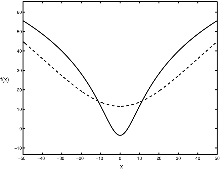
Figure 2: Two-pole solutions of Eq. (65) for $\theta=5$ (full line), and $\theta=10$ (dashed line). Flames propagate downwards.

Equation (65) is derived in the scope of the power expansion with respect to the flame front slope $\phi.$ In the case of the two-pole solution, $|\phi|$ takes its maximal value

$$\phi_{\rm m}=\frac{\theta}{\theta-1}$$

at the points $x_{\rm m}=x_{0}\pm{\rm Im}~{}x_{1}.$ We see that the developed weak nonlinearity expansion is valid if $\theta$ is not too close to unity. For realistic values of the expansion coefficient ($\theta=5-10$) $\phi_{\rm m}\approx 1.$

Next, consider the four-pole solution ($P=2$). It has the form

$$\mathfrak{f}=\frac{\theta(\theta-1)}{2}\ln\left\{\left[(x-{\rm Re}~{}x_{1})^{2}+\left({\rm Im}~{}x_{1}\right)^{2}\right]\left[(x-{\rm Re}~{}x_{2})^{2}+\left({\rm Im}~{}x_{2}\right)^{2}\right]\right\}\,.$$

Assuming that ${\rm Im}~{}x_{1,2}>0,$ one has the following equations for the position of poles $x_{1},$ $x_{2},$ $x_{3}=x_{1}^{*},$ $x_{4}=x_{2}^{*}$

$$i~{}\alpha(\beta+\gamma)+2\left\{\frac{\beta+\gamma}{x_{1}-x_{2}}+(\beta-\gamma)\left(\frac{1}{2i~{}{\rm Im}~{}x_{1}}+\frac{1}{x_{1}-x_{2}^{*}}\right)\right\} = 0\,,$$

$$i~{}\alpha(\beta+\gamma)+2\left\{\frac{\beta+\gamma}{x_{2}-x_{1}}+(\beta-\gamma)\left(\frac{1}{2i~{}{\rm Im}~{}x_{2}}+\frac{1}{x_{2}-x_{1}^{*}}\right)\right\} = 0\,.$$

Separating the real and imaginary parts, and rearranging yields three equations for the four quantities ${\rm Re}~{}x_{1,2}\,,$ ${\rm Im}~{}x_{1,2}$

$$2\alpha\frac{\beta+\gamma}{\beta-\gamma}-\left\{\frac{1}{{\rm Im}~{}x_{1}}+\frac{1}{{\rm Im}~{}x_{2}}+4\frac{{\rm Im}(x_{1}+x_{2})}{|x_{1}-x_{2}^{*}|^{2}}\right\} = 0\,,$$ (68)

$$4~{}\frac{\beta+\gamma}{\beta-\gamma}\frac{{\rm Im}~{}(x_{2}-x_{1})}{|x_{1}-x_{2}|^{2}}+\frac{1}{{\rm Im}~{}x_{2}}-\frac{1}{{\rm Im}~{}x_{1}} = 0\,,$$ (69)

$${\rm Re}(x_{1}-x_{2})\left(\frac{\beta+\gamma}{|x_{1}-x_{2}|^{2}}+\frac{\beta-\gamma}{|x_{1}-x^{*}_{2}|^{2}}\right) = 0\,.$$ (70)

It follows from Eq. (70) that ${\rm Re}~{}x_{1}={\rm Re}~{}x_{2}\,.$ This solution describes the “confluence” of poles. Then the remaining Eqs. (68), (69) give

$${\rm Im}~{}x_{1,2}=\frac{1}{\alpha}\left(1+2~{}\frac{\beta-\gamma}{\beta+\gamma}\right)\left(1\pm\sqrt{\frac{\beta+\gamma}{2\beta}}\right)=\left(\theta^{2}-\theta+1\right)\left(1\pm\sqrt{\frac{2\theta}{\theta^{2}+1}}\right)\,.$$

The two-pole and four-pole solutions are compared in Fig. 3 in the case of $\theta=8$ and $x_{0}=0.$

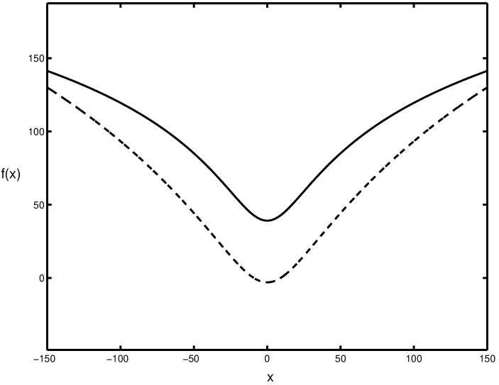
Figure 3: Two-pole (full line) and four-pole (dashed line) solutions of Eq. (65) for $\theta=8.$

The pole confluence is in fact a common property of the solutions (66). To see this, let us take the real part of the equation with $k$ corresponding to the rightmost pole in the upper half-plane. We have

$$\sum\limits_{\genfrac{}{}{0.0pt}{}{l=1}{l\neq k}}^{2P}\left({\rm Re}~{}x_{k}-{\rm Re}~{}x_{l}\right)\frac{\beta\pm\gamma}{|x_{k}-x_{l}|^{2}}=0\,.$$

In view of the choice of $k,$ the left hand side is the sum of non-negative terms. It can be zero only if ${\rm Re}~{}x_{k}-{\rm Re}~{}x_{l}=0$ for all $l.$

The question of which configuration is realized in the given conditions requires carrying out the stability analysis of various pole solutions, and can be solved, of course, only on the basis of the general non-stationary Eq. (III). According to the definition of $\mathfrak{f},$ such an analysis is to be performed with respect to perturbations with wavelengths $\lambda\sim L_{0}.$

IV Discussion and conclusions

The large scale flame dynamics are independent of its local cellular structure in zero order approximation with respect to the flame front thickness. This is the main result of the work, proved in Sec. II. The local flame corrugation only affects the value of the normal velocity $U_{\rm f}$ changing it to $\mathfrak{U}U_{\rm f},$ where $\mathfrak{U}>1$ describes increase of the front length due to its wrinkling. In the scope of the thin front model, $U_{\rm f}$ plays the role of an external parameter specifying the characteristic velocity of the problem under consideration. Thus, the overall effect of the local flame structure on its large scale evolution amounts to a renormalization of this parameter. For flames of practical importance, the $\mathfrak{U}$-factor is about $1.3-1.5.$ In fact, it is $\mathfrak{U}U_{\rm f},$ rather than $U_{\rm f},$ which is more convenient to measure experimentally, since the measurement of $U_{\rm f}$ requires special facilities to suppress development of the LD-instability, such as those used in Ref. clanet .

The decoupling theorem allows one to avoid the difficult issues arising in investigating flame dynamics at length scales of the order $\lambda_{\rm c},$ and to go directly to scales characterizing the problem in question. This is particularly important in numerical simulations of the flame dynamics. The computational grid should be chosen so as to well resolve the flame cellular structure, which leaves a little space for investigation of larger scales because of the limitations of computational facilities.

The decoupling theorem also opens the way for analytical investigation of the large scale flame dynamics. As an example, the nonlinear development of the LD-instability in the presence of the gravitational field was considered in Sec. III, where a weakly nonlinear non-stationary equation for the flame front position was obtained [Eq. (III)]. This equation admits stationary solutions in the case of flame propagation in the direction of the field, which means that the gravitational field has a stabilizing overall effect in this case. The resulting stationary flame configuration turns out to be essentially non-periodic, and represents a symmetrical “hump” in the direction of the flame propagation, with slowly decreasing logarithmic “tails.” A complete investigation of the non-stationary equation will be given elsewhere.

References

• (1) L. D. Landau, “On the theory of slow combustion,” Acta Physicochimica URSS 19, 77 (1944).
• (2) G. Darrieus, unpublished work presented at La Technique Moderne, and at Le Congr${\rm\grave{e}}$s de M${\rm\acute{e}}$canique Appliqu${\rm\acute{e}}$e, (1938) and (1945).
• (3) G. H. Markstein, ”Experimental and theoretical studies of flame front stability,” J. Aero. Sci. 18, 199 (1951).
• (4) P. Pelce and P. Clavin, “Influences of hydrodynamics and diffusion upon the stability limits of laminar premixed flames,” J. Fluid Mech. 124, 219 (1982).
• (5) M. Matalon and B. J. Matkowsky, “Flames as gasdynamic discontinuities,” J. Fluid Mech. 124, 239 (1982).
• (6) G. I. Sivashinsky, “Nonlinear analysis of hydrodynamic instability in laminar flames,” Acta Astronaut. 4, 1177 (1977).
• (7) O. Thual, U. Frish, and M. Henon, ”Application of pole decomposition to an equation governing the dynamics of wrinkled flames,” J. Phys. (France) 46, 1485 (1985).
• (8) G. I. Sivashinsky and P. Clavin, “On the nonlinear theory of hydrodynamic instability in flames,” J. Physique 48, 193 (1987).
• (9) K. A. Kazakov and M. A. Liberman, “Effect of vorticity production on the structure and velocity of curved flames,” Phys. Rev. Lett. 88, 064502 (2002).
• (10) K. A. Kazakov and M. A. Liberman, “Nonlinear equation for curved stationary flames,” Phys. Fluids 14, 1166 (2002).
• (11) Ya. B. Zel’dovich, G. I. Barenblatt, V. B. Librovich, and G. M. Makhviladze, The Mathematical Theory of Combustion and Explosion (Consultants Bureau, New York, 1985).
• (12) K. A. Kazakov and M. A. Liberman, “Nonlinear theory of flame front instability,” Combust. Sci. and Tech., 174, 129 (2002).
• (13) C. Clanet and G. Searby, “First experimental study of the Darrieus-Landau instability,” Phys. Rev. Lett. 80, 3867 (1998).