Analytical solution for nonlinear Schr$\ddot{\hbox{o}}$dinger vortex reconnection

Abstract

Analysis of the nonlinear Schr$\ddot{\hbox{o}}$dinger vortex reconnection is given in terms of coordinate-time power series. The lowest order terms in these series correspond to a solution of the linear Schr$\ddot{\hbox{o}}$dinger equation and provide several interesting properties of the reconnection process, in particular the non-singular character of reconnections, the anti-parallel configuration of vortex filaments and a square-root law of approach just before/after reconnections. The complete infinite power series represents a fully nonlinear analytic solution in a finite volume which includes the reconnection point, and is valid for finite time provided the initial condition is an analytic function. These series solutions are free from the periodicity artifacts and discretization error of the direct computational approaches and they are easy to analyze using a computer algebra program.

PACS number: 67.40.Vs

1 INTRODUCTION

Vortex solutions of the nonlinear Schr$\ddot{\hbox{o}}$dinger (NLS) equation are of interest in nonlinear optics [1, 2, 3] and in the theory of Bose-Einstein condensates [4] (BEC). The NLS equation is also often used to describe turbulence in superfluid helium. [5] NLS is a nice model in this case because the vortex quantization appears naturally in this model and because its large-scale limit is the compressible Euler equation describing classical inviscid fluids. [6, 7] At short scales, the NLS equation allows for a “quantum uncertainty principle” which allows vortex reconnections without the need for a finite viscosity or other dissipation. Numerically, NLS vortex reconnection was studied by Koplik and Levine[8] and, more recently, by Leadbeater et al.[9] and, for a non-local version of NLS equation, by Berloff et al.[4] In applications to superfluid turbulence, the NLS equation was directly computed by Nore et al.[10] Such cryogenic turbulence consists of repeatedly reconnecting vortex tangles, with each reconnection event resulting in the generation of Kelvin waves on the vortex cores [11] and a sound emission. [9] These two small-scale processes are very hard to correctly compute in direct simulations of 3D NLS turbulence due to numerical resolution problems. A popular way to avoid this problem is to compute vortex tangles by a Biot-Savart method (derived from the Euler equation) and use a simple rule to reconnect vortex filaments that are closer than some critical (“quantum”) distance. This approach was pioneered by Schwarz [6] and it has been further developed by Samuels et al.[12] In this case, it is important to prescribe realistic vortex reconnection rules. Therefore, elementary vortex reconnection events have to be carefully studied and parameterized. Numerically, such a study was performed by Leadbeater et al., [9] the present paper is devoted to the analytical study of these NLS vortex reconnection events.

The analytical approach of this paper is based on expanding a solution in powers of small distance from the reconnection point, and small time measured from the reconnection moment. The idea is to exploit the fact that when vortex filaments are near reconnection, the nonlinearity in the NLS equation is small. This smallness of the nonlinearity just stems from the definition of vortices in NLS (curves where $\Psi=0$) and the continuity of $\Psi$. Their core size is of the order of the distance over which $\Psi\rightarrow 1$ (where $\Psi=1$ represents the background condensate). Therefore, for vortices near reconnection, separated by a distance much smaller than their core size, $\Psi$ is small provided it is continuous. Thus, to the first approximation the solution near the reconnection point can be described by a linear solution which, already at this level, contains some very important information about the reconnection process: (1) that the reconnection proceeds smoothly without any singularity formation, (2) that in the immediate vicinity of the reconnection the vortices are strictly anti-parallel and (3) just before the reconnection event the distance between the vortices decreases as $|t|^{1/2}$, where $t$ is the time measured from the reconnection moment. Note that result (1) could surprise those who draw their intuition from vortex collapsing events in the Euler equation (which are believed to be singular). On the other hand, results (2) and (3) are remarkably similar to the numerical and theoretical results found for the Euler equation. [13, 14, 15]

In section II of this paper we examine the local analysis of the reconnection process by deriving a linear solution and in section III consider its properties. The linear solution describes many, but not all the important properties of vortex reconnection. In particular, it cannot describe solutions outside the vortex cores and, therefore, it cannot describe the far-field sound radiation produced by the reconnection. On the other hand, one can substitute the linear solution back into the NLS equation and find the first nonlinear correction to this solution. Recursively repeating this procedure, one can recover the fully nonlinear solution in terms of infinite coordinate and time series. This derivation is discussed in detail in section IV. The series produced are a general solution to a Cauchy initial value problem. Thus, by Cauchy-Kowalevski theorem, [16] these series define an analytic function (with a finite convergence radius) provided the initial conditions are analytic. The generation of such a suitable initial condition is addressed in section V. Our series representation of the solution to the NLS equation is exact, and therefore will include such properties as sound emission. However, due to the finite radius of convergence of the analytic solution, one is unable to observe a far-field sound emission directly. In this paper, we use Mathematica to compute some examples of the fully nonlinear solutions for the vortex reconnection. The results of which are presented in section VI.

Let us summarise the advantages and disadvantages that our analytical solution has with respect to those being computed via direct numerical simulations (DNS). Firstly, our analytical solutions are obtained as a general formula, simultaneously applicable for a broad class of initial vortex positions and orientations. Secondly, our analytical solutions are not affected by any periodicity artifacts (which are typical in DNS using spectral methods) or by discretization errors. On the other hand, our analytical solutions are only available for a finite distance from the vortex lines (of the order of the vortex core size) because their defining power series have a finite radius of convergence.

2 LOCAL ANALYSIS OF THE RECONNECTION

Let us start with the defocusing NLS equation written in the non-dimensional form,

$$i\Psi_{t}+\Delta\Psi+(1-|\Psi|^{2})\Psi=0.$$ (1)

Suppose that in vicinity of the point ${\bf r}=(x,y,z)=(0,0,0)$ at $t=t_{0}$ we have $\Psi=\Psi_{0}$ such that $Re\Psi_{0}=z$, and $Im\Psi_{0}=az+bx^{2}-cy^{2}$, where $a,b$ and $c$ are some positive constants. For such initial conditions the geometrical location of the vortex filaments, $\Psi=0$, is given by two intersecting straight lines, $z=0$ and $y=\pm\sqrt{b/c}\,x$.

In the small vicinity of the point ${\bf r}=0$, deep inside the vortex core (where $\Psi_{0}\approx 0$), we can ignore the nonlinear term found in equation (1). Further, by a simple transformation $\Psi=\Phi e^{it}$ we can eliminate the third term $\Psi$ and obtain $i\Phi_{t}+\Delta\Phi=0$. (This just corresponds to multiplying our solution by a phase, it does not alter its properties, but does make the following analysis simpler). It is easy to see that the initial condition has not changed under this transformation, $\Psi_{0}=\Phi_{0}$. Advancing our system a small distance in time $t-t_{0}$, we find $Re\,\Phi=Re\,\Psi_{0}-(t-t_{0})\,\Delta Im\,\Psi_{0}$ and $Im\,\Phi=Im\,\Psi_{0}+(t-t_{0})\,\Delta Re\,\Psi_{0}$, or

$$Re\,\Phi = z-2(b-c)\,(t-t_{0}),$$ (2)

$$Im\,\Phi = az+bx^{2}-cy^{2}.$$

For both $t-t_{0}<0$ and $t-t_{0}>0$ the set of vortex lines, $\Phi=0$, is given by two hyperbolas. A bifurcation happens at $t=t_{0}$ where these hyperbolas degenerate into the two intersecting lines (see Fig. 1). This bifurcation corresponds to the reconnection of the vortex filaments. Thus, we have constructed a local (in space and time) NLS solution corresponding to vortex reconnection. Obviously, this solution corresponds to a smooth function $\Phi$ at the reconnection point. It should be stressed that this is not an assumption, but just the way in which we have chosen to construct our solution. However, we do believe that this observed smoothness is a common feature of NLS vortex reconnection events. If this is true then all such reconnecting vortices could locally be described by the presented solution as the intersection of a hyperbola with a moving plane provides a generic local bifurcation describing a reconnection in the case of smooth fields.

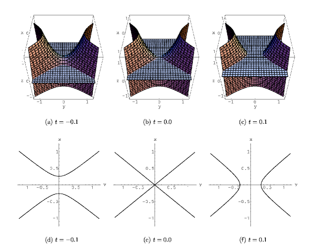
Figure 1: Linear solution Eq. (2) of the nonlinear Schr$\ddot{\hbox{o}}$dinger equation for $a=1$, $b=3$, $c=2$ and $t_{0}=0$. Sub-figures (a), (b) and (c) show the intersection of the real (plane) and imaginary (hyperbolic paraboloid) parts of Eq. (2) at successive times $t=-0.1$, $t=0.0$ and $t=0.1$ respectively. Sub-figures (d), (e) and (f) show the corresponding lines of intersection where $\Psi=0$; reconnection occurs at $t=t_{0}=0$.

3 PROPERTIES OF THE VORTEX RECONNECTION

The local linear solution we have constructed (2) reveals several important properties of the reconnection of NLS vortices.
1. Whatever the initial orientation of the vortex filaments, the reconnecting parts of these filaments align so that they approach each other in an anti-parallel configuration. Indeed, according to (2), the fluid velocity field $\vec{v}=\nabla\arctan([Im\,\Phi]/[Re\,\Phi])=\nabla\arctan([az+bx^{2}-cy^{2}]/[z-2(b-c)(t-t_{0})])$. At the mid-point between the two vortices one finds a velocity field consistent with an anti-parallel pair, $\vec{v}=1/[2a^{2}(c-b)(t-t_{0})]\vec{e}_{z}\neq 0.$ (For a parallel configuration one would find $\vec{v}=0$). Amazingly similar anti-parallel configurations have been observed in the numerical Biot-Savart simulations of thin vortex filaments in inviscid incompressible fluids.[13, 15]
2. The reconnecting parts of the vortex filaments approach each other as $\sqrt{t-t_{0}}$. Indeed, setting $Re\,\Phi=Im\,\Phi=0$ and $y=0$ in (2) one obtains $x=\pm\sqrt{2a[(c/b)-1](t-t_{0})}.$ Exactly the same scaling behaviour, for approaching thin filaments in incompressible fluids, has been given by the theory of Siggia and Pumir [13, 14, 15] and has been observed numerically in Biot-Savart computations. [13, 15]
3. The nonlinearity plays a minor role in the late stages of vortex reconnection in NLS. This is a simple manifestation of the fact that in the close spatio-temporal vicinity of the reconnection point $\Psi\approx 0$, so that the dynamics are almost linear.
This last property can be also reformulated as follows. No singularity is observed in the process of reconnection according to the solution (2): both the real and imaginary parts of $\Psi$ behave continuously in space and time. This property is in drastic contrast to the singularity formation found in vortex collapsing events described by the Euler equation. Indeed, distinct from incompressible fluids, no viscous dissipation is needed for the NLS vortices to reconnect. Here, dispersion does the same job of breaking the topological constraints (related to Kelvin’s circulation theorem) as viscosity does in a normal fluid.

4 NONLINEAR SOLUTION

We will now move on to consider the full NLS equation. We will use a recursion relationship to compute the solution assuming that $x,y,z\sim\epsilon$ and $t\sim\epsilon^{3}$ (for simplicity, we take $t_{0}=0$). The solution we obtain will therefore be of the form $\Psi=\Psi^{(0)}+\Psi^{(1)}+\Psi^{(2)}+\cdots$, where $\Psi^{(n)}\sim\epsilon^{n}$. The above $\epsilon$ scaling of $x$, $y$, $z$ and $t$ has been chosen to generate a recursion relationship when substituted in the NLS equation (1). Of course we could have chosen a different $\epsilon$ dependence, however, as the final series representation of our solution contains an infinite number of terms, this would just correspond to the same solution but with a suitable re-ordering.

Consider the NLS equation (1). Firstly, we note that $\partial_{t}\sim\epsilon^{-3}$ and $\triangle\sim\epsilon^{-2}$ and therefore $i\Psi_{t}^{(m)}\sim\epsilon^{m-3}$, $\triangle\Psi^{(n)}\sim\epsilon^{n-2}$, $\left[|\Psi|^{2}\Psi\right]^{(p)}\sim\epsilon^{p}$ and $\Psi^{(q)}\sim\epsilon^{q}$, where $[|\Psi|^{2}\Psi]^{(p)}=\sum_{i,j=1}^{p}\Psi^{*(i)}\Psi^{(j)}\Psi^{(p-i-j)}$. Matching the terms, by setting $m=n+1$ and $p=q=n-2$, and integrating we find

$$\Psi^{(n+1)}=\Psi_{0}^{(n+1)}+i\int_{0}^{t}\left[\triangle\Psi^{(n)}+\Psi^{(n-2)}-[|\Psi|^{2}\Psi]^{(n-2)}\right]dt,$$ (3)

where $\Psi_{0}^{(n)}$ are arbitrary $n^{th}$ order functions of coordinate which appear as constants of integration with respect to time. The full nonlinear solution of the Cauchy initial value problem can now be obtained by matching $\Psi_{0}^{(n)}$ to the $n^{th}$ order components of the initial condition at $t=0$ obtained via a Taylor expansion in coordinate. Let us assume that the initial condition is an analytic function so that it can be represented by power series in coordinates with a non-zero volume of convergence. Then, by the Cauchy-Kowalevski theorem, the function $\Psi$ will remain analytic for non-zero time. In other words, the solution can also be represented as a power series with a non-zero domain of convergence in space and time. Remarkably, the recursion relation Eq. (3) is precisely the means by which one can write down the terms of the power-series representation of the fully nonlinear solution to the NLS equation, with an arbitrary analytical initial condition $\Psi_{0}$.

5 INITIAL CONDITION

Our next step is to construct a suitable initial condition for our study of reconnecting vortices. This initial condition will have to be formulated in terms of a power series. We start by formulating the famous line vortex solution to the steady state NLS equation [5] in terms of a power series. Substituting $\Psi=Ae^{i\theta}$ into Eq. (1), we find $\triangle A-A|\nabla\theta|^{2}+A-A^{2}=0$, where we have used the fact that $\nabla\theta\cdot\nabla A=0$ and $\triangle\theta=0$. We can simplify this equation, since $A=A(r)$ and therefore, $\triangle A=\frac{1}{r}\partial_{r}(r\partial_{r}A)$. However, we also note that $|\nabla^{2}\theta|=\frac{1}{r^{2}}$ since $\partial_{x}\theta=-y/r^{2}$ and $\partial_{y}\theta=-x/r^{2}$. Therefore, we have $\frac{1}{r}\partial_{r}(r\partial_{r}A)-\frac{A}{r^{2}}-A^{3}+A=0$. We will solve this equation using another recursive method. We would like to get a solution of the form $A=a_{0}+a_{1}r+a_{2}r^{2}+a_{3}r^{3}+\cdots=\sum_{n}A^{(n)}$. (However, we can set $a_{0}$ to zero on physical grounds, since we require $\Psi=0$ at $r=0$). As before $\frac{1}{r}\partial_{r}(rA_{r}^{(m)})=m^{2}a_{m}r^{m-2}\sim\epsilon^{m-2}$, $\frac{A^{(n)}}{r^{2}}=a_{n}r^{n-2}\sim\epsilon^{n-2}$, $[A^{3}]^{(p)}\sim\epsilon^{p}$ and $A^{(q)}=a_{q}r^{q}\sim\epsilon^{q}$, where $[A^{3}]^{(p)}=\sum_{i,j=1}^{p}A^{(i)}A^{(j)}A^{(p-i-j)}.$ Again, by matching powers of $r$ we can derive a recursion relationship for $a_{n}$. Setting $m=n$ and $p=q=n-2$ we obtain

$$a_{n}=(f_{n-2}-a_{n-2})/(n^{2}-1),$$

where $f_{p}=[A^{3}]^{(p)}/r^{p}$.

We should note that $a_{2n}=0$ for all $n$. Therefore, taking a power of r out of our expansion for $A(r)$ we find,

$$\Psi=A(r)r^{i\theta}=rg(r)e^{i\theta},$$

where $g(r)=g(r^{2})=a_{1}+a_{3}r^{2}+a_{5}r^{4}+\cdots=\sum_{n=1}^{\infty}a_{2n-1}r^{2n-2}$. Further, $re^{i\theta}$ is complex so we can write $re^{i\theta}=x+iy$ and hence our prototype solution, for a vortex pointing along the $z$-axis, is $\Psi=(x+iy)g(x^{2}+y^{2})$.

We can manipulate this prototype solution to get an initial condition for our vortex reconnection problem. Our initial condition $\Psi_{0}$ will be made up of two vortices, $\Psi_{1}$ and $\Psi_{2}$, a distance $2d$ and angle $2\alpha$ apart. Following the example of others, [Koplik et al., Ref. Koplik] and [Leadbeater et al., Ref. Leadbeater], we take the initial condition to be the product of $\Psi_{1}$ and $\Psi_{2}$, that is $\Psi_{0}=\Psi_{1}\Psi_{2}$. One could argue that such an initial condition is rather special, as two vortices found in close proximity would typically have already distorted one another in their initial approach. Nevertheless, such a configuration provides us with a valuable insight into the dynamics of NLS vortex reconnections.

Firstly, we would like the vortices in the $(x,y)$ plane. We can do this by transforming our coordinates $x\rightarrow y$, $y\rightarrow z$ and $z\rightarrow x$. This will give us a vortex pointing along the $x$-axis $\Psi=(y+iz)g(y^{2}+z^{2})$. The vortex can now be rotated by angle $\alpha$ to the $x$-axis in the $(x,y)$ plane via $x\rightarrow x\cos\alpha-y\sin\alpha$ and $y\rightarrow y\cos\alpha+x\sin\alpha$. Finally, we shift the whole vortex in the $z$ direction by a distance $d$ using $z\rightarrow z-d$ we finally obtain $\Psi_{1}=[y\cos\alpha+x\sin\alpha+i(z-d)]g((y\cos\alpha+x\sin\alpha)^{2}+(z-d)^{2})$. In a similar manner, $\Psi_{2}$ is a vortex at angle $-\alpha$ and shifted by $-d$ in the $z$ direction, $\Psi_{2}=[y\cos\alpha-x\sin\alpha+i(z+d)]g((y\cos\alpha-x\sin\alpha)^{2}+(z+d)^{2})$.

6 RESULTS

Figure 2: The initial condition for the prototype vortex solution is constructed via an appropriate expansion for $A=A(r)$, Eq. (5). Here we can see the expansion for $A=A(r)$ truncated at three different orders of $n$; $n=5$ (dash-dot line), $n=15$ (dashed line) and $n=21$ (solid line) with $a_{1}=0.6$. At higher orders one would see the existence of a finite radius of convergence at $r\approx 2.5$.

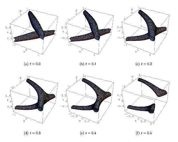
Figure 3: Sub-figures (a) to (f) show the evolution of two initially separated vortices in time $t$. This realization is for $|\Psi|=0.1$, $a_{1}=0.6$, $d=0.6$ and $\alpha=\pi/4$. The reconnection and separation events are clearly evident.

It would time consuming to expand the analytical solution, derived in the previous section, by hand. Thankfully, we can use a computer to perform the necessary algebra, and to derive the hugh number of terms the recursive formulae generate. What follows is an example solution of the reconnection of two initially separated vortices.

Firstly, we need to consider the validity and accuracy of our initial condition. Fig. 2, shows the prototype solution $A=A(r)$ for a single vortex, at various different orders. Increasing the order will obviously improve accuracy. However, one should note that at higher order there is evidence of a finite radius of convergence $r_{c}$. This will restrict the spatial region of validity for our full t-dependent solution. Our prototype solution also has a dependence on $a_{1}$. In the following simulation we have chosen $a_{1}=0.6$ numerically so that the properties of $A(r)$ match that of a NLS vortex. It is evident that we cannot satisfy these properties completely (namely $\Psi\rightarrow 1$ as $r\rightarrow\infty$) as our power series diverges near $r_{c}$. Nevertheless, this does not present us with a problem if we restrict ourselves to considering the evolution of contours of $\Psi$, such as $|\Psi|<1$, where $A(r)$ is realistically represented. Further, it should be noted that sound radiation could in principle be visualized in our solution by drawing contours of $|\Psi|$ close to unity. However, to have an accurate representation, we would need to take a very large number of terms in the series expansion, therefore the study of sound in our model is somewhat harder than the analysis of the vortices themselves. Of course the validity of the full $t$-dependent solution will be restricted, in the spatial sense, by the initial condition’s region of convergence. The region of convergence will evolve, remaining finite during a finite interval of time (by the Cauchy-Kowalevski theorem), but then may shrink to zero afterwards.

We will now discuss an example solution. As we only wish to demonstrate this method, we will not consider a high order solution in this paper. In our example simulation below, we used Mathematica to perform the necessary algebra in generating a nonlinear solution up to $O(\epsilon^{6})$. (One should note that although the prototype solution (5) for a single vortex has $a_{2n}=0$ for all $n$, our initial condition is made up of two vortices, i.e. two series multiplied together. Therefore, there will be cross terms of order $O(\epsilon^{6})$ in our initial condition).

Our choice of parameters will be $d=0.6$ and $\alpha=\pi/4$. This corresponds to two vortices, initially separated by a distance 1.2, at right angles to each other. Fig. 3 shows the evolution of the iso-surface $|\Psi|=0.1$ in time, demonstrating reconnection and then separation. Examining this solution in detail we can clearly see evidence of some of the properties mentioned earlier - that of a smooth reconnection (the absence of singularity) and the anti-parallel alignment of vortices prior to reconnection.

7 CONCLUSION

In this paper we presented a local analysis of the NLS reconnection processes. We showed that many interesting properties of the reconnection can already be seen at the linear level of the solution. We derived a recursion formula Eq. (3) that gives the fully nonlinear solution of the initial value problem in a finite volume around the reconnection point for a finite period of time. In fact, formula (3) can describe a much wider class of problems. Of interest, for example, are solutions describing the creation or annihilation of NLS vortex rings. This process is easily described by considering vortex rings, at there creation/annihilation moment, as the the intersection of a plane with the minimum of a paraboloid. Further, this method of expansion around a reconnection point can be used for other evolution equations, e.g. the Ginzburg-Landau equation. These applications will be considered in future. We wish to thank Robert Indik, Nicholas Ercolani and Yuri Lvov for their many fruitful discussions.

References

- [1] N.N. Akhmediev, Opt. Quan. Elec. 30, 535 (1998).
- [2] A.W. Snyder, L. Poladian and D.J. Mitchell, Opt. Lett. 17 (11) 789 (1992).
- [3] G.A. Swartzlander and C.T. Law, Phys. Rev. Lett. 69 (17), 2503 (1992).
- [4] N.G. Berloff and P.H. Roberts, J. Phys. A 32 (30), 5611 (1999).
- [5] V.L. Ginzburg and L.P. Pitaevskii, Sov. Phys. JETP 7, 858 (1958).
- [6] K.W. Schwarz, Phys. Rev. B. 38 (4), 2398 (1988).
- [7] N. Ercolani and R. Montgomery, Phys. Lett. A. 180, 402 (1993).
- [8] J. Koplik and H. Levine, Phys. Rev. Lett. 71 (9), 1375 (1993).
- [9] M. Leadbeater, T. Winiecki, D.C. Samuels, C.F. Barenghi and C.S. Adams, Phys. Rev. Lett. 86 (8), 1410 (2001).
- [10] C. Nore, M. Abid and M.E. Brachet Phys. Rev. Lett 78 (20), 3896 (1997).
- [11] B.V. Svistunov, Phys. Rev. B 52 (5), 3647 (1995).
- [12] C.F. Barenghi, D.C. Samuels, G.H. Bauer and R.J. Donnelly, Phys. Fluids 9 (9), 2631 (1997).
- [13] A. Pumir and E. Siggia, Phys. Fluids A 2 (2), 220 (1990).
- [14] A. Pumir and E. Siggia, Physica D 37, 539 (1989).
- [15] A. Pumir and E. Siggia, Phys. Rev. Lett. 55 (17), 1749 (1985).
- [16] R. Courant and D. Hilbert, Methods of mathematical physics: partial differential equations 2, (Interscience, London, 1965).