Absolute palaeointensity of Oligocene (28-30 Ma) lava flows from the Kerguelen Archipelago (southern Indian Ocean)–LABEL:lastpage

Absolute palaeointensity of Oligocene (28-30 Ma) lava flows from the Kerguelen Archipelago (southern Indian Ocean)

We report palaeointensity estimates obtained from three Oligocene volcanic sections from the Kerguelen Archipelago (Mont des Ruches, Mont des Tempêtes, and Mont Rabouillère). Of 402 available samples, 102 were suitable for a palaeofield strength determination after a preliminary selection, among which 49 provide a reliable estimate. Application of strict a posteriori criteria make us confident about the quality of the 12 new mean-flow determinations, which are the first reliable data available for the Kerguelen Archipelago. The Virtual Dipole Moments (VDM) calculated for these flows vary from 2.78 to 9.47 10²² Am² with an arithmetic mean value of 6.15$\pm$2.1 10²² Am². Compilation of these results with a selection of the 2002 updated IAGA palaeointensity database lead to a higher (5.4$\pm$2.3 10${}^{22}Am^{2}$) Oligocene mean VDM than previously reported [Goguitchaichvili et al., 2001, Riisager, 1999], identical to the 5.5$\pm$2.4 10${}^{22}Am^{2}$ mean VDM obtained for the 0.3-5 Ma time window. However, these Kerguelen palaeointensity estimates represent half of the reliable Oligocene determinations and thus a bias toward higher values. Nonetheless, the new estimates reported here strengthen the conclusion that the recent geomagnetic field strength is anomalously high compared to that older than 0.3 Ma.

1 Introduction

Numerous studies have been carried out to increase our knowledge of geodynamo physics, but even so we still do not know the detailed mechanism of the generation of the Earth’s magnetic field, and even less about the processes that produce secular variation, excursions and reversals (e.g., Jacobs Jacobs94; Merrill & McFadden Merrill99). To better understand the geomagnetic field we need to be able to go back in time in order to observe its changes and to obtain long-term global characteristics. This is possible with some rocks which recorded the Earth’s palaeomagnetic field during their formation. Volcanic rocks, in particular, furnish a global knowledge of the geomagnetic field because they contain information on both the direction (inclination and declination) and the strength of the palaeofield. However, the most reliable methods for absolute palaeointensity determination, Thellier & Thellier Thellier59 and its modified version proposed by Coe Coe67a, are time consuming because of the strict conditions which have to be checked to validate the determinations. Moreover, many volcanic rocks turn out to be unsuitable for palaeointensity determination. For these reasons, reliable palaeointensity data are difficult to obtain and are particularly rare. Only 1.5 determinations per million years between 0 and 300 Ma [Selkin & Tauxe, 2000] are available when combining the updated IAGA 1999 data-set and the Scripps submarine basaltic glass databases. It is obvious that more palaeointensity data are needed for a better understanding of the geomagnetic dynamo.
This study on three basaltic sections sampled in the Kerguelen Archipelago (49.9S, 70E) aims to estimate more accurately the palaeomagnetic strength of the geomagnetic field in the 28-30 Ma time interval recorded by these lavas. It thus complements the palaeomagnetic directions recently published on the same sections  [Plenier et al., 2002]. By combining these new determinations with selected records issued from preexisting palaeomagnetic databases (Tanaka et al. Tanaka95, updated by Perrin & Shcherbakov Perrin97 and Perrin et al. Perrin98a) we will propose a more robust estimation of the Oligocene palaeofield strength and we will discuss the long-term characteristics of the geodynamo.

2 Geology and sampling

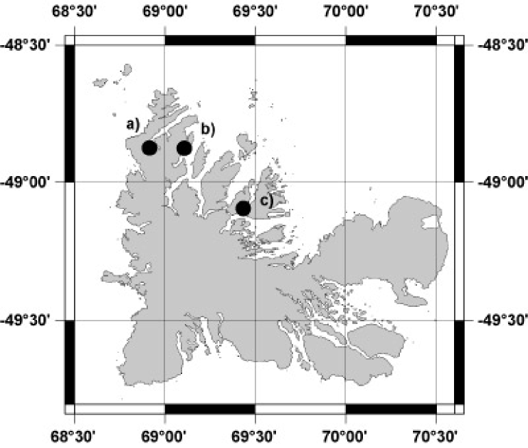
Figure 1: Location of the studied sections: a) Mont des Ruches : 18 flows (4852’18”S, 6854’48”E), b) Mont des Tempêtes : 20 flows (4852’50”S, 6906’37”E), c) Mont Rabouillère : 19 flows (4905’25”S, 6926’25”E).

The Kerguelen Archipelago lies on the northern part of the Kerguelen-Gaussberg Plateau (southern Indian Ocean). This archipelago is the subaerial continuation of Kerguelen hotspot volcanism for the last 30 Ma  [Yang et al., 1998, Weis et al., 1998, Nicolaysen et al., 2000]. The lava flows form the tabular reliefs (400 to 900 m high) observed today after glacial erosion, and represent more than 85% of the archipelago surface [Giret, 1990]. The rest of the archipelago is composed of intrusions (gabbro, granite, and syenite) issued from Kerguelen plume melts [Weis & Giret, 1994] and quaternary glacial sediments. We studied paleomagnetic cores collected along three vertical sections of Kerguelen basalt at Mont des Ruches, Mont des Tempêtes, and Mont Rabouillère sections (Fig. 1). For the reasons developed in Plenier et al. Plenier02, the palaeomagnetic sections do not correspond exactly to the previously-dated sections [Yang et al., 1998, Nicolaysen et al., 2000, Doucet et al., 2002], but they appear to be correlated. Usually, we drilled seven samples in each successive lava flow using a gas-powered drill and oriented them with both solar sightings and magnetic compass with a clinometer. We took care to sample the bottom part of the least altered flows, and as far away as possible from intrusions.

3 Rock magnetism and sample selection

For field intensities comparable to those of the Earth’s magnetic field (few tens of $\mu$T), there is a proportionality between the Thermo-Remanent Magnetization (TRM) intensity measured at 20C and the strength of the ancient magnetic field present during cooling through the blocking temperatures for almost all natural rocks. Thus, for some particular rocks cooling in the geomagnetic field during their formation, it is possible to estimate the palaeomagnetic field strength recorded by comparing their Natural Remanent Magnetization (NRM) with an artificial TRM acquired in the laboratory under a known ambient field. However, the coefficient of proportionality depends on grain size, shape distribution, and blocking temperatures as well as on the amount and type of ferromagnetic material the rock contains. In addition, this coefficient may have changed since the formation of the rock or during heating in the laboratory. For this last reason, a procedure using numerous successive heatings with increasing temperature steps has been developed [Thellier & Thellier, 1959] in order to limit the field strength estimates to the temperature range preceding the irreversible magnetic and/or chemical changes in the ferromagnetic minerals. The strict conditions to be respected by the samples for correct palaeointensity determination are the following:

1. The Characteristic Remanent Magnetization (ChRM) recorded by the studied specimen has to be a TRM, acquired at a known epoch in the geomagnetic field.

2. The ChRM should not be disturbed by significant secondary magnetizations.

3. The physical, chemical and crystallographical properties of the magnetic minerals must not have changed since the initial TRM was acquired nor changed during the successive heatings imposed by the experimental method.

4. The independence and additivity laws of partial-TRM (pTRM) enunciated by Thellier Thellier38 have to be satisfied. That is, the total TRM must be equivalent to a sum of pTRMs, each associated with its own blocking temperature interval and not dependent on the remanence carried in every other intervals. This generally means that the magnetic carriers have to be single domain (SD) or in favorable cases pseudo-single domain (PSD) grains.

It is obvious that numerous samples can not fulfill these conditions, thus extensive preliminary studies are necessary to avoid unnecessary work.

3.1 Viscosity indices and demagnetizations

We shown recently [Plenier et al., 2002] by means of a positive reversal test that the ChRM measured from Kerguelen lava are, generally speaking, not disturbed by unremoved secondary components and then that these ChRMs are primary TRMs. In order to assess the importance of the secondary component carried by each sample, we analyzed the results from demagnetization experiments performed previously on sister specimens [Plenier et al., 2002].
First, we rejected samples for which the angle between the NRM and the ChRM was greater than 15 and those contaminated by a resistant secondary component (e.g., unremoved beyond 20 mT alternating fields treatment or 300C when samples are demagnetized by heating in zero field). Likewise, we kept only those flows for which the NRMs of all samples were well grouped. 60% of the flows fulfilled these conditions. For these flows, only the samples with a demagnetization curve as undisturbed as possible and presenting unblocking temperatures as high as possible, or median-demagnetization field of at least 20 mT, were retained.
Second, we estimated the capacity of the specimens to gain a secondary Viscous Remanent Magnetization (VRM) by measuring them first after two weeks in the ambient magnetic field oriented along the z core axis and again, after two-week storage in a zero field. This enables determination of the viscosity index [Thellier & Thellier, 1944] for each sample, which are reported in Table 1. The viscosity index corresponds to about 25% of the VRM acquired in situ since the last reversal 780 ky ago [Prévot, 1981]. We choose the arbitrarily thresholds for the viscosity index of 10% as an upper limit for specimen from intermediate polarity flow and 5% for the others [Prévot et al., 1985].

3.2 Susceptibility at room temperature and k-T curves

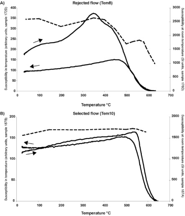
Figure 2: Low-field susceptibility versus temperature curves: continuous measurements at temperature k-T (solid line) and room temperature measurements k₀-T (dashed line) curves of a rejected (A) and a selected (B) flow.

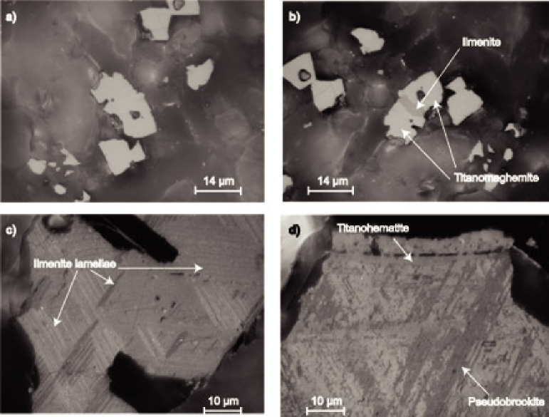
Figure 3: Reflected light microphotographs using an oil immersion objective. a),b): sample 269b (Tou2) in natural light shown in different orientations in order to illustrated the pleochroic ilmenite associated with a non pleochroic phase which could correspond to a titanomaghemite; c),d): two characteristic minerals from sample 234c (Tem16) in polarized light. The crossed nicols are at 90

To be sure of the thermal stability of the samples during successive heating in the laboratory, we used the low-field magnetic susceptibility (k₀) measured at room temperature after each thermal demagnetization step performed in air for the sister specimen previously studied in the palaeodirection determination [Plenier et al., 2002]. A favorable sample for palaeointensity determination should have a relatively constant k₀ value during most of the demagnetization procedure. However, this is not a sufficient criterion because thermally unstable samples may nonetheless display low variations in the susceptibility measured at room temperature. Thus to complete this approach, we measured continuously the low-field susceptibility of one sample from each flow usually during two successive heating-cooling cycles under vacuum, the first up to 350C and the second up to the Curie temperature (Tc). Fig. 2 presents two representative k-T curves (susceptibility as a function of temperature) encountered during this study. The first case (Fig. 2a) illustrates the irreversible and complex thermomagnetic behaviour observed for almost 60% of the samples. The magnetic carriers are interpreted as original titanomagnetite associated with titanomaghemite, a product of their low temperature oxidation. We rejected the flows yielding this behaviour because of their thermal instability. The second case (Fig. 2b) illustrates the reversible behaviour observed for the rest of the samples. The magnetic carriers are low-Ti titanomagnetites probably produced by high temperature oxyexsolution of the original titanomagnetites. We considered flows presenting this second reversible behaviour as suitable for palaeointensity determination experiments.
In order to complement this thermomagnetic investigation, we observed thin sections from each k-T curve type using an oil immersion objective. Fig. 3a and  3b show photomicrographs in natural light of sample 269b (flow Tou2), which displayed irreversible behaviour. We saw an isotropic phase sometimes associated with a pleochroic ilmenite, as illustrated here. Because titanomagnetite and titanomaghemite are difficult to distinguish under the microscope, it is hard to conclude about the nature of the isotropic phase. These two minerals are certainly both present, but the existence of cracks almost omnipresent in this phase suggest a larger amount of titanomaghemite. This interpretation agrees well with the irreversible k-T curve. Fig. 3c and  3d show two minerals from a thermally stable sample (234c, flow Tem16). They illustrate two different advanced stages of deuteric oxidation with ilmenite or titanohematite lamellae exsolved from a residual titanomagnetite almost entirely altered. Again this observation confirms the interpretation of the k-T curves.

3.3 Pilot analysis

We kept only flows for which at least three samples from different cores fit all the previously enumerated criteria for the palaeointensity experiments (32 out of the initial 57). We performed a pilot analysis with one or two samples from each of these flows in order to identify the most favorable flows for reliable determinations and to define the more appropriate demagnetization steps for the next series. After applying a posteriori criteria which will be presented later, 5 flows from the Mont des Ruches section, 9 from the Mont des Tempêtes section and 1 from the Mont de la Rabouillère section seemed suitable. Because a sample which did not pass all the a priori selection criteria may sometimes furnish a reliable determination [Coe, 1967b, Perrin, 1998], they should be regarded as serving only for selecting the most appropriate flows for palaeointensity determination. For this reason, the remaining samples from the suitable flows underscored by the pilot analysis have been incorporated in the following two determination series (68 specimens), including the samples which did not pass all the a priori criteria first.

4 palaeointensity experiments

4.1 Experimental procedure

We used the method of Thellier & Thellier Thellier59 in its classical form to estimate the palaeointensity of the geomagnetic field. We also followed a sliding pTRM checks procedure [Prévot et al., 1985] every two demagnetization steps in order to verify that the pTRM capacity remains unaltered when the heating temperature is progressively increased. Because of the nonlinearity of acquisition of TRM in multidomain grains [Levi, 1977], applying a laboratory field far from the recorded one may lead to underestimate the ancient field [Coe, 1967b, Tanaka & Kono, 1984]. Thus, to improve the quality of data, we took care to apply, along the vertical axis of the samples, a constant field of 50 $\mu$T (known with a precision of 0.1 $\mu$T), which corresponds approximately to the strength of the mean Oligocene field for Kerguelen latitude. We also carried out the heating-cooling cycles under a vacuum better than 10^-4 mbar to limit possible oxidation during experiments. We performed demagnetizations up to 580C, with 13 steps ranging from 50 to 10C, using a home made furnace (temperature reproduced within 2C) in the palaeomagnetic laboratory of the University of Montpellier. Before the treatment, and after each heating-cooling cycle, we measured the remanence with a JR5-A spinner magnetometer. To ensure the reproducibility of the procedure at the same demagnetization step (pair of heating-cooling cycles and pTRM check), we always kept the specimens in the same place in the oven.

4.2 Preliminary selection of palaeointensity data

Because the interpretation of palaeointensity experiments is subjective, as many other data interpretations, a posteriori criteria help to ensure the technical quality and objectivity of the results and their comparison from study to study. It is noteworthy to point out that except the number of data used for each individual determination, which has been fixed to four consecutive points, the other a posteriori criteria were not used directly to reject a determination. When only one or two a posteriori criteria failed, we kept the determination choosing the nearest temperature interval for which the corresponding criteria stay as close as possible from the exclusion bounds fixed. The data with more than three independent criteria unfulfilled have been considered as unable to furnish a reliable palaeointensity estimate and thus have been excluded.

1. $f$ criterion: A classical way of representing palaeointensity data is to use the Arai diagram [Arai, 1963, Nagata et al., 1963] in which the NRM_T remaining at each temperature step T is plotted against the pTRM_T acquired in the laboratory field from T to room temperature. The slope of the least squares fit line computed from the linear part of the NRM-pTRM diagram gives an estimate of the palaeofield strength. Thus criteria have to be defined to constrain the determination of this best fit line and to quantify its technical quality.
   We already fixed the minimum number of successive points used for the determinations to four. The other criteria used is the NRM fraction $f$ given by the ratio of the NRM lost over the selected temperature interval to the total NRM [Coe et al., 1978]. We consider that a value of 0.3 is the minimum NRM fraction for acceptable determination. Note that a quality factor $q$ [Coe et al., 1978, Prévot et al., 1985] less than 5 can also indicate a determination of the palaeofield strength of poor quality. However, because $q$ is not independent of $f$, this lead to reject the same samples in this study. Thus we did not use it as a rejection criterion.
   

2. Control on vector endpoint diagrams (Zijderveld’s plot): Because a straight line in the Arai plot can involve more than one component, we checked their existence on the Zijderveld’s projection of the NRM demagnetization computed from the palaeointensity experiments. To complete this qualitative approach, we quantified the dispersion of the points regarding to the best fit line by the maximum angular deviation (MAD) [Kirschvink, 1980] and chose a maximum value of 10 for this criterion.
   Another quality criterion is given by the angle $\alpha$ between the best fit line (anchored to the center of mass) and the vector average (anchored to the origin) of the selected data in the Zijderveld plot. If the data correspond to the primary remanence, $\alpha$ should be inferior to say 10, in the opposite, they are certainly biased by a spurious unknown component.
   

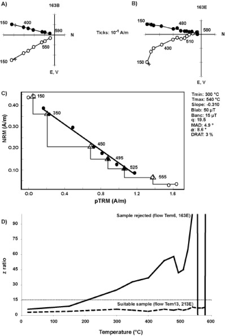
Figure 4: Illustration of the a posteriori criteria used to select sample. A) Orthogonal projection of the sister specimen demagnetization, B) Orthogonal projection of the studied sample demagnetization, calculated from the palaeointensity experiment, C) NRM-TRM diagram of the same specimen, and D) Evolution of its z ratio compared to the evolution of the suitable sample 213E.

3. $z$ ratio: The heating remanent magnetizations (HRM) [Calvo et al., 2002] acquired during the heating procedure under the application of a constant weak field in palaeointensity experiments, lead to erroneous data. Hopefully, the direction along which the laboratory field was applied corresponds to the axis of our cylindrical samples (Z axis). Therefore, in a Zijderveld plot in sample coordinates, the acquisition of HRM appears as a progressive deviation of the demagnetization curve in the vertical plane towards the vertical axis direction. This is illustrated in Fig. 4 in which we compare the Zijderveld’s plot inferred from the palaeointensity experiment for a rejected sample with the demagnetization curve of its sister specimen obtained during the palaeodirection analysis.
   An ”HRM check” is allowed using the ratio [Goguitchaichvili et al., 1999a]:

   $$\mathrm{z=\frac{HRM_{T}}{NRM_{T}}\times 100\%}$$ (1)

   where $\mathrm{HRM_{T}}$ and $\mathrm{NRM_{T}}$ are the HRM created in the sample and the NRM left in the ChRM direction, at a given temperature T, respectively. Similar ratios exist (e.g. R or R’ [Coe et al., 1984]) but the $z$ ratio allows to monitor the evolution of alterations during treatment. Calculating this ratio supposes that one knows the ChRM direction, which requires demagnetization of a sister specimen before the palaeointensity experiment.
   To help the interpretation, we defined the upper limit of the accepted temperature interval as the one preceding a $z$ >20%. However, we extended the interval over this limit when the ratio NRM left/TRM gained did not change in the new interval. In this case some magneto-chemical transformations are present but do not change the estimate. A limitation of the $z$ ratio is that it depends on the angle between the ChRM and the applied field direction (direction of the HRM). The more this angle tends to 90, the bigger is the deviation. Unfortunately, the tray we used to place the specimens in the oven did not permit us to orient their ChRM at 90 to the applied field. Hence, the $z$ we calculated is a minimum value, thus these steps had to be rejected. Another limitation of this criterion is that some unexpected fluctuations may appear at high temperature when the NRM left is too small. For this reason, we completed this approach by observing the evolution of the demagnetization on an equal area projection. In Fig. 4, the $z$-T curve of a rejected sample 163E (Tem06) is compared to the one obtained from an accepted sample (213E, flow Tem13).

4. Difference ratio (DRAT): We performed sliding pTRM checks in order to estimate the temperature at which alteration of the magnetic minerals begins. Commonly, many authors consider that repeated pTRM acquisition at the same temperature steps should agree to within 15% [Goguitchaichvili et al., 1999b]. However, pTRMs acquired within low-temperature interval, are rather small and thus a reproducibility within a given percentage is difficult to obtain. Therefore, we used the difference ratio (DRAT) [Selkin & Tauxe, 2000], which normalizes the maximum difference between repeated pTRM steps performed on the temperature interval selected for the determination by the length of the corresponding NRM-pTRM segment. We fixed a maximum acceptable value of 10% for this criterion. However, this ratio reveals possible alterations on the estimate interval only, whereas physical and chemical alterations of the heated samples can appear as soon as the first demagnetization steps [Kosterov & Prévot, 1998]. Therefore, we also monitored the lower temperature pTRM checks by determining the DRAT from ambient to maximum temperature of the interval used to estimate the palaeointensity. It is noteworthy that the sample 163E (Fig. 4), rejected because of its $z$ ratio, has a DRAT of only 3%. Also five samples which give an estimate in Table 4 possess a DRAT >10%, thus these two alteration criteria are complementary.
   

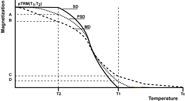
Figure 5: Continuous thermal demagnetization of pTRM(T₁,T₂). The low-temperature pTRM-tail for PSD (A) or MD (B) grains corresponds to the part of pTRM(T₁,T₂) removed at T₂, while the high-temperature pTRM-tail corresponds to the part of this pTRM unremoved at T₁, (C) for MD and (D) for PSD grains. The low and high-temperature pTRM-tails are measured at room temperature.

5. High temperature pTRM-tail test: Unfortunately, 56% of the samples present a more or less pronounced curvature in their NRM-TRM diagrams and some specimens provide two acceptable estimates regarding the selection criteria. Because independence and additivity laws of pTRM [Thellier, 1938] are violated for MD but maybe also for PSD grains, the determination of the domain structure could be a relevant tool to choose between the two acceptable palaeointensity estimates.
   In case of thermally stable samples, we used the thermomagnetic criterion that was first introduced by Bol’shakov & Shcherbakova  Bolshakov79 to get insight on the domain structure of ferrimagnetics. We calculated the parameter $\mathrm{A_{HT}}$ which is illustrated in Fig. 5 and defined by:

   $$\mathrm{A_{HT}(T_{1},T_{2})=\frac{tail_{HT}[pTRM(T_{1},T_{2})]}{pTRM(T_{1},T_{2})}\times 100\%}$$ (2)

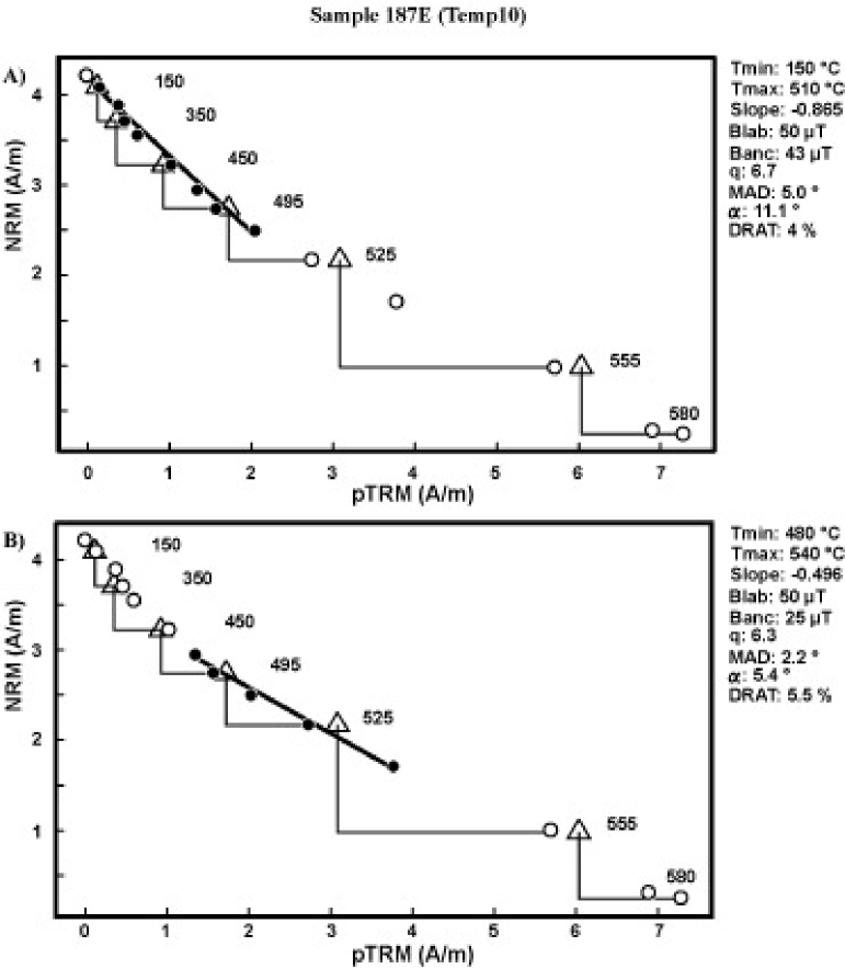
Figure 6: Arai diagram for sample 187E (flow Tem10) illustrating a case for which two acceptable interpretations are possible. A) The low-temperature interval is rejected regarding the pTRM-tail test (Table 2) which favours the high-temperature interval determination shown in B). Black (White) circles are the step used (not used) for the palaeointensity estimate, the triangles represent the pTRM checks.

   where $\mathrm{pTRM(T_{1},T_{2})}$ is the pTRM measured at room temperature gained between T₁ and T₂ ($\mathrm{T_{1}<T_{2}}$) during cooling from the Curie temperature (T_c) in a 100$\mu$T field, and the $\mathrm{tail_{HT}[pTRM(T_{1},T_{2})]}$ is the part of this pTRM not demagnetized when the sample is subsequently heated again to T₁ and cooled down is zero field. According to the criteria defined by Shcherbakova et al. Shcherbakova00 for $\mathrm{A_{HT}(T_{1},T_{2})}$ <4%, the remanent carrier are predominantly SD grains, for 4% <$\mathrm{A_{HT}(T_{1},T_{2})}$ <(15-20)%, they behave as pseudo-single domain (PSD) grains, and for $\mathrm{A_{HT}(T_{1},T_{2})}$ >20% they are predominantly MD grains.
   We measured the coefficients $\mathrm{A_{HT}(T_{1},T_{2})}$ at increasing temperature intervals for one thermally stable sample per flow in order to determine the best temperature interval to estimate the paleointensity. Because the heatings were performed in air, we repeated the determination of the coefficient $\mathrm{A_{HT}(300,T_{room})}$ two times, at the beginning and at the end of the treatment, in order to monitor alterations appearing during the successive heatings. Unfortunately, the vibrating thermal magnetometer (VTM) we used broke before we could measure all the representative samples of each selected flow. The results available are reported in Table 2. Even though all the flows have not been studied, the global trend observed confirms that with increasing temperature, the magnetic carrier behaviour is more SD-like [Carvallo et al., 2003, Shcherbakova et al., 2000]. Thus, when two coexisting palaeointensity estimates remain possible (5 samples), the high temperature pTRM-tail test favors acceptance of the higher temperature interval determination, as for sample 187E shown in Fig. 6.
   

6. Low temperature pTRM-tail test: According to Fabian Fabian01, the pTRM tail is not a direct measure for a sample’s tendency to yield a curved Arai plot. The common concave-up shape of MD Arai diagrams is rather well accounted for by the low temperature tail (Low-T tail) of each pTRM segment acquired during cooling from Tc ($\mathrm{pTRM_{LT}(T_{1},T_{2})}$). This Low-T tail is due to the grains with unblocking temperature less than blocking temperature. In order to compare the results obtained from the two tail tests and validate the choice of the temperature intervals for the interpretation, we decided to evaluate the Low-T tail of some characteristic samples used during the palaeointensity experiment. We define the coefficient:

   $$\mathrm{A_{LT}(T_{1},T_{2})=\frac{tail_{LT}[pTRM(T_{1},T_{2})]}{pTRM(T_{1},T_{2})}\times 100\%}$$ (3)

   where $\mathrm{pTRM(T_{1},T_{2})}$ is the pTRM measured at room temperature gained between T₁ and T₂ ($\mathrm{T_{1}<T_{2}}$) in a 50$\mu$T field during cooling from the Curie temperature and $\mathrm{tail_{LT}[pTRM(T_{1},T_{2})]}$ is the part of this pTRM removed when the sample is subsequently heated to T₂ and cooled down in zero field (Fig. 5). This coefficient is analogous to the $\mathrm{A_{HT}}$ coefficient defined by Shcherbakov et al. Shcherbakov01b but the relation between the magnitude of the two tails is not clear. We can expect from Dunlop & Özdemir Dunlop01 that $\mathrm{A_{LT}}$ is equal to $\mathrm{A_{HT}}$ because the unblocking temperature distributions are almost symmetric for a given blocking temperature, but this may be quite different for hundred-degree temperature intervals. In the absence of a quantitative study, only the evolution of the $\mathrm{A_{LT}}$ ratio for increasing temperature intervals will be considered.
   The $\mathrm{A_{LT}}$ coefficients for the (450,350) and (550,450) temperature intervals are reported in Table 3. The main result is that $\mathrm{A_{LT}(550,450)}$ is always smaller than $\mathrm{A_{LT}(450,350)}$; thus the Low-T tail test again favors the higher temperature interval in case of two acceptable determinations. In order to estimate the alteration which may occur during the required preliminary heating up to T_c, the untreated samples 187D and 201C have been incorporated in the experiment. Comparing their results with the data from the corresponding sister samples 187E and 201E, we can observe that, even though these samples appear thermally stable (reversible k-T curves), $\mathrm{A_{LT}(450,350)}$ is greater for the sample used in the palaeointensity estimate and on the contrary $\mathrm{A_{LT}(550,450)}$ is greater for the ”virgin” sample. Nonetheless, for the five samples that allowed two acceptable interpretations, we choose the higher temperature interval, which yields determination more coherent with the other samples from the same flow.

4.3 Palaeointensity results

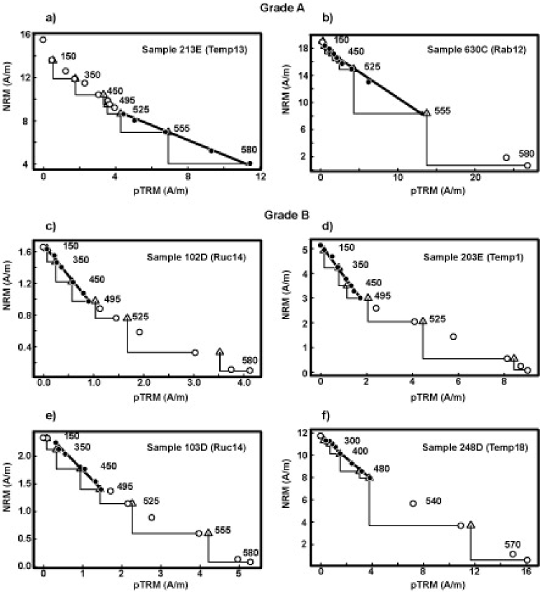
Figure 7: Characteristic examples of palaeointensity estimates from this study. a) and b) correspond to grade A estimates, c), d), e) and f) to grade B estimates. Black (White) circles are the step used (not used) for the palaeointensity estimate, the triangles represent the pTRM checks.

Out of the 402 samples from the Mont des Ruches, Mont des Tempêtes, and Mont Rabouillère sections, 102 have been chosen using a priori criteria. After selection following a posteriori criteria, 49 samples furnish a technically acceptable determination (Table 4).
The quality factor q varies from 1.6 to 54.3 with a mean value of 12.1 for estimates made on a mean of 7 points. However, some $\alpha$ angles are relatively large, which could be due to an overprint of viscous origin, even though the samples are not strongly viscous, or to a secondary component acquired during the treatment, as shown by the angle $\beta$ between the ChRMs of the sample and its sister specimen. Although secondary HRM exists, we consider its effect negligible on the determination, considering the $z$ criterion, the linearity of the Arai diagram and the evolution of the demagnetization in an equal area projection. Therefore, as evidenced by the MAD, which is the most widely satisfied a posteriori criterion, we are confident about these interpretations. Moreover, as is commonly done in palaeointensity studies, we distinguished two types of determination: class A for the samples which passed successfully all the criteria and class B for those in which one to three criteria were unfulfilled. However, as observed with flows Rab12 or Tem6, there is no single relation between the field estimate and its classification. Thus, the interpretations made with a few unsatisfied a posteriori criteria can be also considered as reliable. Fig. 7 shows some characteristic examples of palaeointensity determinations.
We present, in Table 4, the mean palaeofield strength with its associated standard deviation for each individual flow. Three consecutive Mont des Ruches flows (Ruc14, 15, and 16) yield a well defined palaeointensity in the range 35-40 $\mu$T. This value is comparable with the only reliable flow from the Mont Rabouillère section (Rab12) and with the flows Tem13 and Tem15 from the Mont des Tempêtes. For this last section we also observe three significantly higher values around 50-60 $\mu$T (Tem1,17 and 18) and two well defined lower field strengths of only 20.1 and 25.0$\pm$1.7 $\mu$T (Tem6 and 10). Because, the within flow standard deviation represent at the maximum 15% of the palaeointensity value (flow Tem13), we are quite confident about the reliability of these estimations.
We performed in a previous study [Plenier et al., 2002], a quantitative bootstrap test for a common mean on successive magnetic directions in order to identify non-independent records. We concluded in particular that the Ruc14 and Ruc15 flows may represent two contemporaneous records of the palaeofield (Table 1). The palaeointensity estimates obtained for these two successive flows overlap within their uncertainties and thus strengthen our former interpretation. However, because the palaeomagnetic field may remain constant for a relatively long time [Love, 2000] we will nevertheless consider in the present study each of the 12 reliable palaeointensity estimates as distinct records.
Concerning the samples 101F, 111F, 201E, 160E, 161F and 229C, for which pTRM-tail tests were performed, we decided to keep the lower rather than the higher temperature interval estimates because the latter was sometimes impossible to define owing to alteration of the pTRM blocking temperature spectra (101F, 160E, 201E and 229C) or meaningless compared to the other determinations from the same flow (111F, 161F).

5 Discussion

5.1 Toward an improvement of palaeointensity determination

Because of the strict conditions imposed by the commonly used palaeointensity determination method of Thellier & Thellier Thellier59, numerous checks are needed to ensure reliable estimates. For this reason, palaeointensity experiments are time consuming and at the end many samples do not furnish reliable determinations. Consequently, the number of reliable estimates is very low and studies dealing with palaeointensity determinations are relatively rare. Then, effective selection followed by careful palaeointensity determination method are desirable to increase the productivity of the experiments and largely implement the number of palaeointensity estimates in the databases.
However, no ideal selection criteria exist to select suitable specimens and flows for palaeointensity experiments. For example, Sherbakov et al. Shcherbakov01b proposed to use a pTRM-tail check as a systematic procedure before the experiments to discriminate the samples with MD grains. The few determinations of the low and high temperature pTRM-tail performed in the present study are not convincing since many samples yielding a paleointensity estimate with good technical quality (Table 4) will not have been kept if we followed Shcherbakov et al.’s Shcherbakov01b recommendation. Thus, we do not recommend to use the thermomagnetic criterion for selection but rather in a case to case basis to define the best temperature interval for thermally stable specimens exhibiting two slopes in the NRM/TRM diagram. For the selection based on k-T curve shapes, the temperature intervals used for the estimates (c.f. Table 4) can change at the flow scale (flow Tem13 or Tem15) without important deviation in the palaeofield strength. Therefore, the thermal behaviour of the samples varies within a flow and this criterion applied to a supposedly representative sample is not totally effective.
A study of each successful sample, at the end of the palaeofield strength determination procedure, up to the maximum temperature reached for the palaeointensity estimate would be more interesting. Whatever the numerous a priori precautions we took in this study, only 48% of the selected samples gave a reliable estimate. Thus, in the absence of relevant a priori criteria, it is preferable to reduce the preliminary experiments to the determination of the viscosity index, which is an already rapid and reliable way to discriminate the specimens disturbed by a viscous secondary component, followed by a directional analysis, needed for careful palaeointensity estimates and giving enough information to discard possibly problematic flows because of large NRM scatter, poor technical quality of demagnetization curves and so on.
As regard to the determination procedure itself, some modifications of the Thellier’s method have been proposed recently  [Calvo et al., 2002, Riisager & Riisager, 2001]. They include an additional heating at each demagnetization step in order to control the HRM creation and/or a “pTRM tail check”. However, the lack of suitable selection criteria lead to more failure of the palaeointensity experiment and these more time consuming procedures are consequently not helpful for systematic studies. Orienting the samples so that their ChRM is perpendicular to the direction of the applied field is less time consuming and sufficient to check for possible HRM creation. Likewise, at the end of the treatment, complementary experiments like k-T curve shape determination, extended Thellier’s method [Fabian, 2001] for thermally stable samples or ”pTRM tail checks” can be performed to ensure the quality and sharpen the reliable estimates, but such supplementary processes must concern the acceptable samples only. Thus, good determinations do not necessarily need supplementary heatings nor burdensome procedures to be performed; this should be limited only to the problematic samples. Reducing the selection and placing the control procedures at the end of the treatment is thus a way to perform reliable palaeointensity estimates more quickly, without lowering the quality of the determinations.

5.2 Comparison with previous palaeointensity results

Five Oligocene flows from the Ile Haute section (49.4S, 69.9E) have been processed for palaeointensity study  [Derder et al., 1990]. Of the 24 samples analyzed, 11 yielded a determination, but only one flow provided more than three estimates of the palaeofield strength. Moreover, the uncertainty of the mean palaeointensity is equal to 36% and consequently, these data cannot be considered as reliable. The 12 distinct mean flow estimates presented in this paper are thus the only reliable determinations available for the Kerguelen Archipelago.
However, data well distributed on the Earth’s surface are needed to provide a correct idea of the palaeomagnetic field behaviour. It is then important to pool the Oligocene Kerguelen results with other reliable determinations already achieved. For this aim, we used the updated IAGA 2002 palaeointensity database available at the following address:

ftp://ftp.dstu.univ-montp2.fr/pub/paleointdb/

This database presents estimates obtained with different quality determinations. However, inclusion of lower quality data leads to higher average values of the geomagnetic field [Juarez & Tauxe, 2000, Goguitchaichvili et al., 1999b], thus a selection using identical criteria to those used in this study is needed before we can combine them meaningfully with the Kerguelen results. For this reason we discarded estimates based on intermediate polarity flows, obtained with other methods than the Thellier & Thellier’s  Thellier59 associated with pTRM checks, presenting less than 3 individual samples from the same unit (except for basaltic submarine glasses) and a standard deviation of the mean $\geq$20%. Application of these drastic selection criteria led to the rejection of 660 determinations out of the 910 estimates contained in the database between 0.3 and 50 Ma (Fig. 8a). Then we sharpened the selection to a time window between 20 and 40 Ma, which resulted in 11 suitable estimates among the 74 initial extended Oligocene records of the data base (Fig. 8a).
In order to compare the Kerguelen determinations with the selected estimates issued from various locations and recording different time, we calculated the virtual dipole moment (VDM) given by:

$$\mathrm{VDM=\frac{4\pi R^{3}}{\mu_{0}}F_{ancient}(1+3\cos^{2}\theta)^{-1/2}}$$ (4)

which corresponds to the moment of a dipole field producing the estimated palaeointensity $\mathrm{F_{ancient}}$ at the magnetic colatitude $\theta$. R is the Earth radius. Results of the calculations are reported in Table 4 and the 12 suitable determinations are plotted in Fig. 8.
Even though we performed careful estimates in order to avoid any possible MD effects in the interpretations, which could lead to systematic higher determinations, the arithmetic mean obtained with the Kerguelen data, 6.15$\pm$2.1 10${}^{22}Am^{2}$, is definitely higher than the other Oligocene estimates already achieved  [Goguitchaichvili et al., 2001, Riisager, 1999, Juarez et al., 1998]. Including Kerguelen determinations leads to an increase of the Oligocene mean VDM from 4.1$\pm$0.5 to 5.4$\pm$2.3 10${}^{22}Am^{2}$. The new Oligocene mean VDM is closer to the mean VDM estimated for the 0.3 and 5 Ma interval [Juarez & Tauxe, 2000] and higher than the mean VDM defined between 0.3 and 300 Ma (Fig. 8). Thus these selected Oligocene estimates favor a relatively stable field between 0.3 and 40 Ma and reinforce the idea of an exceptionally high recent geomagnetic field strength. However, the lack of good palaeointensity data didn’t allow us to go further in our interpretation. As illustrated in Fig. 8c, the Oligocene data do not uniformly cover the Earth’s surface even though the Kerguelen results equalize the number of estimates available for each hemisphere. More reliable determinations are needed to better constrain the evolution of the palaeofield with geological time. It is important to note that the Kerguelen results represent half of the reliable palaeointensity estimates available for the Oligocene, which could lead to a bias towards higher values. Moreover, only 3 extended Oligocene determinations are from normal polarity flows. Thus even if the 12 new estimates are supposed to be independent, the Oligocene palaeomagnetic field may not be sufficiently time-averaged.

6 Conclusion

We carried out a palaeointensity study on three Oligocene (28-30 Ma) volcanic sections from the Kerguelen Archipelago (southern Indian Ocean). It complements the palaeosecular variation directional study already achieved on the same sections: Mont des Ruches, Mont des Tempêtes, and Mont Rabouillère  [Plenier et al., 2002]. Out of the 57 studied units, we considered 32 suitable for palaeofield strength determination experiments when at least three of their samples pass the following selection criteria: angle between NRM and ChRM $\leq 15\degr$ (or secondary component quickly demagnetized), NRM dispersion not too large, viscosity index <5 %, stable susceptibility at room temperature after each demagnetization step of a sister sample and reversible susceptibility in temperature curves. After preliminary experiments, we studied all samples from 12 favorable flows. We considered only the determinations made with at least 4 successive steps, a $z$ ratio [Goguitchaichvili et al., 1999a] $\leq 20$%, a DRAT [Selkin & Tauxe, 2000] $\leq 10$%, f factors [Coe et al., 1978] $\geq 0.3$, a MAD $\leq 10\degr$ [Kirschvink, 1980] and an angle $\alpha$ between the best fit line and the vector average $\leq 10\degr$ to be of good technical quality. In cases of two acceptable estimates, pTRM tail tests were used to choose the temperature interval corresponding to the more SD like behaviour. This careful interpretation of the data leads to 49 reliable estimates. The VDMs calculated for the 12 flows vary from 2.78 to 9.47 with an arithmetic mean value of 6.15$\pm$2.1 10${}^{22}Am^{2}$. This study gives the first reliable palaeointensity estimates from the Kerguelen Archipelago and significantly increases the number of Oligocene data of comparable quality. The new Oligocene mean VDM calculated, 5.4$\pm$2.3 10${}^{22}Am^{2}$, is very close to the 0.3-5 Ma value of Juarez & Tauxe Juarez00 (5.5$\pm$2.4 10${}^{22}Am^{2}$), and suggests little evolution of the geomagnetic field between 0.3 and at least 40 Ma. Thus the present moment of the field (8 10${}^{22}Am^{2}$) is confirmed to be exceptionally high. However, the lack of reliable data limits the interpretation and we discuss practical solutions to speed the selection of suitable samples for careful determination procedures in order to facilitate systematic studies and increase existing palaeointensity databases with high-quality estimates.

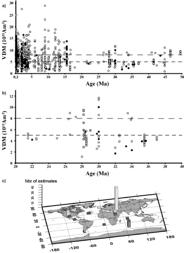
Figure 8: a) black(open) circles are selected(unselected) VDMs from the IAGA 2002 updated data-set between 0.3 and 50 Ma. Gray squares are the data from this study which pass the selection criteria. Long (short) dashed line indicates the 0-0.3 Ma (0.3-300 Ma) mean VDM value. b) same as a) but for the extended Oligocene (20-40 Ma) time window. c) Location of the palaeointensity records between 20 and 40 Ma. Dark(light) gray column are selected(unselected) estimates from the IAGA 2002 updated data-set for the time window considered.

Table 1: Cleaned average directions of magnetization of lava flows retained for paleointensity experiments from Plenier et al. (2002).

Flow	Chron	n/N	Inc		Dec		$\alpha_{95}$		$\kappa$		Plat		Plong		$\nu$%		Alt
Mont des Ruches section (48.87$\degr$S, 68.91$\degr$E)
Ruc16	C9r	4/4	79.	9	183.	3	6.	5	201.	6	-68.	4	65.	9	2.	48	180
Ruc15(1)	C9r	7/7	74.	5	159.	2	3.	9	244.	8	-73.	1	105.	3	4.	60	160
Ruc14(1)	C9r	7/7	76.	4	149.	5	4.	5	183.	8	-67.	7	104.	5	5.	80	150
Mont des Tempêtes section (48.88$\degr$S, 69.11$\degr$E)
Tem18	C9r	8/8	60.	7	177.	0	3.	5	248.	7	-82.	5	231.	6	2.	73	172
Tem17	C9r	7/7	62.	0	186.	0	4.	0	224.	8	-83.	0	287.	7	3.	36	160
Tem16	C9r	5/7	64.	2	178.	1	4.	2	328.	6	-86.	8	224.	6	5.	57	152
Tem15	C9r	4/4	64.	5	188.	1	2.	8	1109.	8	-84.	0	317.	3	4.	04	145
Tem13	C9r	7/7	55.	5	180.	5	5.	0	146.	0	-77.	2	250.	9	2.	99	130
Tem10	C9r	7/7	60.	6	188.	0	7.	0	75.	6	-80.	8	289.	7	2.	56	105
Tem6	C9r	5/5	77.	1	221.	2	2.	4	979.	6	-63.	0	31.	9	4.	94	75
Tem1	C10n.1n	7/7	-67.	3	356.	6	2.	8	464.	7	87.	5	309.	2	5.	87	5
Mont Rabouillère section (49.09$\degr$S, 69.44$\degr$E)
Rab12	C10r	7/7	68.	2	140.	2	4.	2	207.	0	-64.	8	138.	7	1.	80	150
${}^{(\textit{1})}$ indicates flows which have been grouped together in Plenier et al.’s (2002) directional analysis. Flows are listed in stratigraphic order with the youngest on top, oldest on the bottom. Chron correspond to the polarity chrons inferred from Plenier et al.’s (2002) analysis. n/N is the number of samples analyzed/total number of samples collected. Inc and Dec are the mean inclination, positive downward, and the declination east of north, respectively. $\alpha_{95}$ is the 95% confidence envelope for the average direction. $\kappa$ is the precision parameter of Fisher distribution. Plat/Plong is the latitude/longitude of VGP position, respectively. $\nu$% is the geometric mean viscosity index [Thellier & Thellier, 1944]. Alt is the altitude of the flow in meter.

Table 2: High-temperature pTRM-tail test

Flow	Sample	300-Troom	400-300C	500-400C	550-500C	300-T${}_{room}^{*}$
		AHT (B)	AHT (B)	AHT (B)	AHT (B)	AHT
Ruc16	117B	17.0	34.6	n.d.	n.d.	n.d.
Ruc15	111C	48.8 (9.7)	48.1 (11.5)	30.6 (23.3)	13.9 (55.5)	50.7
Ruc14	101C	20.8 (11.7)	29.8 (7.5)	13.3 (27.9)	4.0 (52.9)	17.3
Ruc10	076B	25.2 (40.6)	33.1 (18.1)	32.7 (12.9)	6.8 (28.4)	20.3
Tem13	216C	14.4 (11.4)	30.1 (9.9)	9.5 (32.4)	10.3 (46.3)	21.1
Tem10	187B	23.9 (10.4)	25.5 (10.7)	11.6 (31.8)	5.0 (47.1)	21.3
	189B	29.8 (10.1)	34.1 (7.3)	21.7 (19.1)	5.3 (63.5)	26.4
Tem6	160B	32.8 (14.9)	17.4 (16.6)	28.6 (20.1)	11.5 (48.4)	30.7
Tem1	201B	12.4 (17.5)	15.5 (3.0)	16.6 (21.3)	3.7 (58.2)	8.8
Rab10	620D	15.2 (17.1)	35.0 (6.7)	11.4 (34.8)	7.6 (41.4)	16.8
AHT values are the relative intensities measured at room temperature of the high temperature pTRM-tail expressed in percent $\mathrm{A(T_{1},T_{2})=tail[pTRM(T_{1},T_{2})]/pTRM(T_{1},T_{2})}$. B values shown in parentheses correspond to the percent of the total pTRM (e.g., $\mathrm{\sum_{i}pTRM_{i}}$) each pTRM(T1,T2) represents; nd means not determined. ∗ is a pTRM-tail test (300-Troom) repeated at the end of the treatment to control the thermal stability of the sample. For $\mathrm{A_{HT}(T_{1},T_{2})}$ <4%, the remanent carriers are predominantly SD grains, for 4% <$\mathrm{A_{HT}(T_{1},T_{2})}$ <(15-20)%, they present a PSD behaviour, and for $\mathrm{A_{HT}(T_{1},T_{2})}$ >20% they are predominantly MD grains.

Table 3: Low-temperature pTRM-tail test

Flow	Sample	450-350C	550-450C
		ALT (B)	ALT (B)
Tem18	251C	15.7 (9.0)	2.9 (64.6)
Tem16	237E	8.2 (9.3)	2.0 (74.1)
Tem15	229C	12.3 (9.4)	5.1 (59.8)
	230D	7.3 (8.2)	3.1 (43.2)
Tem13	213E	6.9 (7.6)	2.3 (31.8)
	214D	23.5 (7.7)	3.9 (18.8)
	215F	3.6 (8.1)	3.4 (22.6)
	217D	5.7 (6.5)	2.9 (43.4)
Tem10	187E	13.0 (7.0)	2.3 (65.1)
	187D	8.8 (7.2)	2.4 (54.8)
	189E	12.9 (5.1)	2.3 (57.9)
Tem6	161F	3.8 (11.7)	1.5 (42.9)
Tem1	201E	18.3 (3.3)	2.2 (72.0)
	201C	10.1 (6.3)	2.4 (73.9)
$\mathrm{A_{LT}(T_{1},T_{2})}$ are the relative intensities measured at room temperature of the part of the pTRM(T1,T2) removed after heating to T2 in zero field. B values shown in parentheses correspond to the percent of the total TRM (pTRM(580,$T_{room}$)) each pTRM(T1,T2) represents.

Table 4: Palaeointensity determinations

Flow	Spl	Grade	Fe$\pm$$\sigma$Fe		$\Delta$T	n	f	g	q	MAD	$\alpha$	$\beta$	DRAT	F̄e$\pm$s.d.		VDM
Ruc16	115C	B	34.0 $\pm$	1.4	20-400	5	0.32	0.72	5.5	6.2	(11.7)	7.9	0.7	34.8 $\pm$	0.9	4.69
	116C	B	34.2 $\pm$	2.6	150-400	4	(0.22)	0.58	1.6	3.5	7.9	5.7	0.4
	117F	B	34.8 $\pm$	2.2	150-400	5	(0.23)	0.62	2.2	2.2	7.5	3.0	4.1
	118F	B	36.3 $\pm$	1.3	20-400	5	0.32	0.68	6.2	1.7	(16.6)	14.8	3.5
Ruc15	108C	B	43.0 $\pm$	2.9	20-400	5	(0.25)	0.73	2.7	4.2	8.8	7.8	0.4	40.0 $\pm$	4.3	5.69
	110E	B	37.8 $\pm$	1.1	350-540	8	0.37	0.81	10.2	4.4	(19.8)	16.7	4.1
	111F	B	45.0 $\pm$	1.1	20-400	6	(0.23)	0.79	4.9	4.6	11.2	10.8	1.7
	114D	B	34.2 $\pm$	0.9	150-480	6	0.53	0.79	15.9	1.8	(16.4)	11.0	5.2
Ruc14	101F	B	38.6 $\pm$	1.1	20-480	8	0.37	0.81	10.8	4.1	(15.7)	12.9	2.7	37.2 $\pm$	2.7	5.18
	102D	B	39.6 $\pm$	1.0	150-495	7	0.39	0.80	12.6	2.5	(12.2)	10.5	2.4
	103D	B	33.5 $\pm$	1.8	300-495	6	0.33	0.75	4.5	2.2	(12.1)	5.9	8.1
Tem18	245D	A	65.4 $\pm$	2.1	20-510	9	0.44	0.86	11.8	4.2	8.2	2.6	5.5	55.0 $\pm$	6.9	9.30
	246C	B	43.9 $\pm$	0.8	300-495	6	(0.27)	0.78	11.5	2.7	(18.2)	10.1	7.6
	248D	B	51.6 $\pm$	1.8	150-500	8	(0.29)	0.82	7.2	5.7	(13.0)	10.0	4.2
	249D	A	53.0 $\pm$	4.2	20-400	5	0.36	0.71	3.2	2.6	7.3	1.9	0.1
	251C	A	54.8 $\pm$	1.5	150-525	9	0.51	0.85	15.8	3.2	4.9	3.9	4.1
	252D	B	61.2 $\pm$	1.6	20-495	8	0.52	0.81	16.0	3.0	(10.1)	6.4	(13.8)
Tem17	238D	B	48.4 $\pm$	2.5	150-495	7	(0.28)	0.82	4.5	3.4	(14.7)	11.5	5.7	51.8 $\pm$	6.8	8.62
	239D	B	58.8 $\pm$	2.1	150-480	6	(0.25)	0.78	5.4	5.1	(19.4)	14.0	(10.1)
	240E	B	39.2 $\pm$	0.9	150-500	8	0.40	0.79	13.1	5.1	(11.1)	5.7	5.3
	241D	B	56.6 $\pm$	1.1	150-495	7	0.36	0.82	15.1	3.3	(12.5)	7.2	6.3
	243E	B	57.3 $\pm$	3.5	150-450	5	(0.23)	0.73	2.7	4.9	(26.3)	27.5	6.6
	244E	B	50.3 $\pm$	0.9	150-510	8	0.35	0.84	16.0	5.0	(10.1)	5.2	2.2
Tem16	232D	A	35.2 $\pm$	0.8	20-540	11	0.54	0.87	20.8	2.8	8.0	1.0	4.2	30.5 $\pm$	3.8	4.95
	233C	B	30.4 $\pm$	0.4	350-540	8	0.69	0.84	40.5	2.3	2.5	1.9	(10.7)
	234E	B	24.6 $\pm$	0.4	300-540	9	0.73	0.84	35.3	3.4	1.3	3.0	(15.1)
	237E	A	31.6 $\pm$	0.6	350-540	6	0.54	0.66	18.1	2.5	1.5	4.3	2.3
Tem15	228D	A	34.3 $\pm$	0.8	480-580	8	0.76	0.76	25.3	3.1	1.8	2.6	7.7	36.6 $\pm$	1.6	5.89
	229C	B	38.2 $\pm$	1.7	150-495	7	0.30	0.82	5.4	7.2	(17.5)	13.4	2.1
	230D	A	37.1 $\pm$	0.4	480-580	6	0.78	0.71	54.3	1.6	0.3	5.1	5.8
Tem13	213E	A	32.8 $\pm$	1.0	525-580	5	0.41	0.72	9.8	2.2	0.9	2.8	2.0	39.7 $\pm$	5.7	7.18
	214D	A	34.7 $\pm$	1.7	20-555	12	0.48	0.85	8.1	3.5	5.8	6.5	2.5
	215F	A	36.6 $\pm$	1.5	20-555	12	0.58	0.85	12.4	5.1	2.2	4.6	2.4
	216F	A	40.0 $\pm$	1.9	20-500	9	0.52	0.85	9.1	7.8	8.5	4.0	5.4
	217D	A	45.9 $\pm$	3.3	20-555	12	0.74	0.85	8.7	1.9	3.3	2.7	3.2
	218C	A	48.3 $\pm$	3.1	20-555	12	0.50	0.82	6.3	3.5	6.4	7.3	5.2
Tem10	187E	A	24.8 $\pm$	1.0	480-540	5	0.35	0.71	6.3	2.2	5.4	2.5	5.5	25.0 $\pm$	1.7	4.23
	188E	A	27.2 $\pm$	1.4	510-555	4	0.47	0.53	4.8	4.1	4.7	3.2	5.1
	189E	A	23.0 $\pm$	0.5	525-570	4	0.66	0.62	17.5	3.4	1.1	6.3	6.1
Tem6	160E	B	21.4 $\pm$	0.5	20-500	9	0.57	0.83	21.4	9.4	(14.9)	6.7	6.0	20.1 $\pm$	1.7	2.78
	161F	A	21.2 $\pm$	0.9	150-525	9	0.53	0.85	10.6	3.6	6.0	2.8	4.0
	162E	B	17.8 $\pm$	0.5	20-525	10	0.52	0.80	16.7	(10.6)	(14.0)	6.1	5.5
Tem1	201E	B	55.9 $\pm$	4.9	150-480	7	0.31	0.82	2.9	6.1	(16.9)	13.2	1.8	61.0 $\pm$	3.6	9.47
	203E	B	62.9 $\pm$	2.6	20-495	8	0.42	0.84	8.6	3.8	(11.0)	9.8	7.3
	205E	B	64.1 $\pm$	3.2	150-510	8	0.35	0.82	5.7	4.7	9.9	6.6	(13.1)
Rab12	628B	A	35.5 $\pm$	0.6	225-500	7	0.53	0.77	24.4	3.3	5.7	4.3	5.2	37.7 $\pm$	2.4	5.76
	629B	A	38.0 $\pm$	2.0	150-480	7	0.54	0.75	7.7	2.1	8.1	5.2	7.1
	630C	A	41.4 $\pm$	1.1	150-555	11	0.57	0.72	7.8	2.2	5.8	6.7	1.5
	631C	B	35.8 $\pm$	1.6	150-450	5	0.30	0.68	4.5	5.3	(16.1)	11.9	3.3
Grade: classification based on the number of a posteriori criteria checked (A all, B except at least one evidenced with parenthesis); Fe$\pm$$\sigma$Fe: individual palaeofield strength determination (in $\mu$T) and standard error associated [Prévot et al., 1985]; $\Delta$T: temperature interval of determination; n: number of consecutive points used for the determination; f, g and q: fraction of NRM, gap factor and quality factor, respectively [Coe et al., 1978, Prévot et al., 1985]; MAD: maximum angular deviation; $\alpha$: angle between ChRM and origin; $\beta$: angle between ChRMs of the sample and its sister specimen [Plenier et al., 2002]; DRAT: difference ratio  [Selkin & Tauxe, 2000]; F̄e$\pm$s.d.: mean palaeofield strength of the flow and the standard deviation associated; VDM: virtual dipole moment (*$10^{22}Am^{2}$).