Evaluation of the two-photon exchange diagrams for the $\bf(1s)^{2}2p_{3/2}$ electron configuration in Li-like ions

Abstract

We present ab initio calculations of the complete gauge-invariant set of two-photon exchange graphs for the $(1s)^{2}2p_{3/2}$ electron configuration in Li-like ions. These calculations are an important step towards the precise theoretical determination of the $2p_{3/2}$-$2s$ transition energy in the framework of QED.

I Introduction

At present the lowest-lying states in heavy Li-like ions can be investigated very precisely both theoretically and experimentally. One of the most precise experimental results in these systems has been obtained by Beiersdorfer and co-workers beiersdorfer98 for the $2p_{3/2}$-$2s$ transition energy in Li-like bismuth, which was determined with an accuracy of $0.04$ eV. Accurate experimental data are available at present for a number of other elements as well. For the latest high-precision measurements we refer to Refs. bosselmann99 ; feili00 ; brandau00 ; the outline of earlier investigations can be found in Ref. bosselmann99 .

The accuracy reached in experimental investigations provides a promising tool for probing QED corrections in the strong Coulomb field of the nucleus up to second order in the fine structure constant $\alpha$. For the $2p_{1/2}$-$2s$ transition, this project has been carried out in a series of our previous investigation artemyev99 ; yerokhin99 ; yerokhin00 ; yerokhin01pra2p . In Ref. yerokhin01pra2p we completed the evaluation of all two-electron QED corrections of second order in $\alpha$ and obtained most accurate theoretical predictions for the $2p_{1/2}$-$2s$ splitting within a wide range of nuclear charge numbers $Z$. Based on a careful estimate of the uncertainty of the theoretical values, we concluded that already now the comparison of theory and experiment for Li-like uranium provides a test of QED effects of second order in $\alpha$ at the level of accuracy of about 17%. For the $2p_{3/2}$-$2s$ and $2p_{1/2}$-$2s$ transitions in Li-like bismuth, analogous calculations have been performed recently by Sapirstein and Cheng sapirstein01 . However, in order to match with the experimental accuracy for the $2p_{3/2}$-$2s$ splitting, rigorous evaluations of second-order QED corrections are required also for other ions than bismuth. The first step in this direction has been performed in our earlier investigation artemyev99 where we have evaluated the vacuum-polarization screening correction for several energy levels of Li-like ions, including the $(1s)^{2}2p_{3/2}$ state. The aim of the present work is to calculate the two-photon exchange correction for this state (for extensive calculations of these corrections for the lower states in Li-like ions and for non-mixed low-lying states in He-like ions we refer the reader to Refs. yerokhin00 ; yerokhin01pra2p ; blundell93b ; lindgren95pra ; moh00 ; and01 ; and02 ). After all that, the self-energy screening correction remains the last uncalculated two-electron second-order QED contribution for this state.

This paper is organized as follows. In the next section we present the basic formulas for the two-photon exchange correction for the $(1s)^{2}2p_{3/2}$ state. The description of our numerical procedure is given in Sec. III, and the results obtained are discussed in Sec. IV.

Relativistic units ($\hbar=c=1$) are used throughout this paper.

II Basic formulas

The detailed derivation of the two-photon exchange corrections to the $(1s)^{2}2s$ and $(1s)^{2}2p_{1/2}$ states of Li-like ions can be found in our previous paper yerokhin01pra2p . For the $(1s)^{2}2p_{3/2}$ state the derivation is performed along the same lines. Thus, we present mainly the final formulas here. Our derivation is based on the two-time Green function (TTGF) method shabaev90ivf ; shabaev94ttg2 . For the detailed description of the method we refer to the recent review shabaev02rep .

The two-photon exchange corrections to the $(1s)^{2}2p_{3/2}$ state of the Li-like ions can be conveniently separated in three parts: the two-photon exchange contribution due to the interaction between two $1s$ electrons, the two-photon exchange contribution due to the interaction between the valence electron and one of the $1s$ electrons, and the three-electron contribution. The first part coincides with the two-photon exchange correction to the ground-state energy of He-like ions. Its calculation was carried out in blundell93b ; lindgren95pra . This correction does not contribute to the $2p$-$2s$ splitting in Li-like ions and is not considered here. The remaining two-electron and three-electron corrections are diagrammatically depicted in Fig. 1.

We start from the expression for the second-order correction to the energy shift of the level $k$ shabaev02rep ,

$$\Delta E^{(2)}_{k} = \frac{1}{2\pi i}\oint_{\Gamma}dE\,\Delta E\,\Delta g^{(2)}_{kk}(E)$$ (1)

$$- \frac{1}{2\pi i}\oint_{\Gamma}dE\,\Delta E\Delta g^{(1)}_{kk}(E)\frac{1}{2\pi i}\oint_{\Gamma}dE^{\prime}\,\Delta g^{(1)}_{kk}(E^{\prime})\,,$$

where $\Delta g_{kk}(E)=g_{kk}(E)-g_{kk}^{(0)}(E)$, $g_{kk}(E)=\langle u_{k}|g(E)|u_{k}\rangle$, $u_{k}$ is the unperturbed wave function, $\Delta E=E-E_{k}^{(0)}$, $E_{k}^{(0)}$ is the unperturbed energy of the state $k$, and $g_{kk}^{(0)}(E)=(\Delta E)^{-1}$ is the function $g_{kk}(E)$ in the zeroth-order approximation. The function $g(E)\equiv g(E,{\bf x}_{1}^{\prime},\cdots,{\bf x}_{N}^{\prime};{\bf x}_{1},\cdots,{\bf x}_{N})$ is the temporal Fourier transform of the N-electron two-time Green function. Its definition and the corresponding Feynman rules can be found in shabaev02rep . The superscripts in Eq. (1) indicate the order of the contribution in $\alpha$.

For the two-photon exchange correction, Feynman diagrams contributing to $\Delta g^{(2)}(E)$ are presented in Fig. 1. We refer to the corresponding contributions as the ladder (a), the crossed (b), and the three-electron (c) terms. The second term in Eq. (1) is known as the disconnected contribution. It vanishes completely when considered together with the reducible contribution (for details, see yerokhin01pra2p ). In our case, the unperturbed wave function is

$$u_{k}=\frac{1}{\sqrt{3!}}\sum_{P}(-1)^{P}\psi_{Pa}({\bf x}_{1})\psi_{Pb}({\bf x}_{2})\psi_{Pv}({\bf x}_{3})\,,$$ (2)

where $v$ denotes the valence electron, $a$ and $b$ are the electrons in $(1s)^{2}$ shell, and $P$ is the permutation operator (in the factor $(-1)^{P}$, the parity of the permutation is implied by $P$). For brevity we will use also the following notations:

$$I(\omega) = e^{2}\alpha^{\mu}\alpha^{\nu}D_{\mu\nu}(\omega)\,,$$ (3)

$$I_{abcd}(\omega) = \langle ab|I(\omega)|cd\rangle\,,$$ (4)

$$I_{ab;cd} = I_{abcd}(\Delta_{bd})-I_{bacd}(\Delta_{ad})\,,$$ (5)

$$I^{\prime}(\omega) = \frac{dI(\omega)}{d\omega}\,,$$ (6)

where $\Delta_{ab}=\varepsilon_{a}-\varepsilon_{b}$, $\alpha^{\mu}=(1,{\mbox{\boldmath$\alpha$}})$ are the Dirac matrices, and $D_{\mu\nu}(\omega)$ is the photon propagator.

We separate the contributions of the diagrams under consideration into two parts: the reducible, with the energy of the intermediate state coinciding with the energy of the initial (final) state, and the irreducible, for the remainder, respectively. Omitting the derivation similar to that in Ref. yerokhin01pra2p , we present here only the final expressions for the energy shift. The reducible (”red”) and irreducible (”ir”) three-electron contributions read

$$\Delta E_{\rm ir}^{\rm 3el} = \sum_{PQ}(-1)^{P+Q}$$ (7)

$$\times \sum_{n}\,^{\prime}\frac{I_{P2P3nQ3}(\Delta_{P3Q3})\,I_{P1nQ1Q2}(\Delta_{Q1P1})}{\varepsilon_{Q1}+\varepsilon_{Q2}-\varepsilon_{P1}-\varepsilon_{n}}\,,\,\,\,\,\,\,\,\,\,\,$$

$$\Delta E_{\rm red}^{\rm 3el} = \sum_{\mu_{a}}\biggl{[}I^{\prime}_{vaav}(\Delta_{va})(I_{ab;ab}-I_{bv;bv})$$ (8)

$$+ \frac{1}{2}I^{\prime}_{av\tilde{v}b}(\Delta_{va})I_{b\tilde{v};av}+\frac{1}{2}I^{\prime}_{b\tilde{v}va}(\Delta_{va})I_{va;\tilde{v}b}\biggr{]}\,,$$

where $P$ and $Q$ are the permutation operators, and the prime in the sum in Eq. (7) indicates that terms with the vanishing denominator should be omitted in the summation. In Eq. (8) $a$ and $b$ denote $1s$ electrons with opposite angular-momentum projections $\mu_{a}=-\mu_{b}$, $v$ stands for the valence state with the angular-momentum projection $\mu_{v}$, and $\tilde{v}$ is the valence state with $\mu_{\tilde{v}}=2\mu_{a}+\mu_{v}$ (the corresponding contribution is assumed to be zero when $\mu_{\tilde{v}}$ is out of the range $-j_{v},\ldots,j_{v}$).

The irreducible two-electron contribution is

$$\Delta E^{\rm 2el}_{\rm"ir"} = \Delta E^{\rm lad}_{\rm dir}+\Delta E^{\rm lad}_{\rm exch}+\Delta E^{\rm cr}_{\rm dir}+\Delta E^{\rm cr}_{\rm exch}\,,$$ (9)

$$\Delta E^{\rm lad}_{\rm dir} = \sum_{n_{1}n_{2}}\!{}^{\prime}\frac{i}{2\pi}\int_{-\infty}^{\infty}d\omega$$ (10)

$$\times \frac{F^{\rm lad}_{\rm dir}(\omega,n_{1}n_{2})}{(\varepsilon_{c}-\omega-\varepsilon_{n_{1}}u)(\varepsilon_{v}+\omega-\varepsilon_{n_{2}}u)}\,,$$

$$\Delta E^{\rm lad}_{\rm exch} = -\sum_{n_{1}n_{2}}\!{}^{\prime}\frac{i}{2\pi}\int_{-\infty}^{\infty}d\omega$$ (11)

$$\times \frac{F^{\rm lad}_{\rm exch}(\omega,n_{1}n_{2})}{(\varepsilon_{v}-\omega-\varepsilon_{n_{1}}u)(\varepsilon_{c}+\omega-\varepsilon_{n_{2}}u)}\,,$$

$$\Delta E^{\rm cr}_{\rm dir} = \sum_{n_{1}n_{2}}\!{}^{\prime}\frac{i}{2\pi}\int_{-\infty}^{\infty}d\omega$$ (12)

$$\times \frac{F^{\rm cr}_{\rm dir}(\omega,n_{1}n_{2})}{(\varepsilon_{c}-\omega-\varepsilon_{n_{1}}u)(\varepsilon_{v}-\omega-\varepsilon_{n_{2}}u)}\,,$$

$$\Delta E^{\rm cr}_{\rm exch} = -\sum_{n_{1}n_{2}}\!{}^{\prime}\frac{i}{2\pi}\int_{-\infty}^{\infty}d\omega$$ (13)

$$\times \frac{F^{\rm cr}_{\rm exch}(\omega,n_{1}n_{2})}{(\varepsilon_{v}-\omega-\varepsilon_{n_{1}}u)(\varepsilon_{v}-\omega-\varepsilon_{n_{2}}u)}\,.$$

Here we introduced the labels ”lad” and ”cr” for the ladder and the crossed diagram, and ”dir” and ”exch” for the direct and the exchange parts. The other notations are:

$$F^{\rm lad}_{\rm dir}(\omega,n_{1}n_{2}) = \sum_{\mu_{c}\mu_{n_{1}}\mu_{n_{2}}}I_{cvn_{1}n_{2}}(\omega)I_{n_{1}n_{2}cv}(\omega)\,,$$ (14)

$$F^{\rm lad}_{\rm exch}(\omega,n_{1}n_{2}) = \sum_{\mu_{c}\mu_{n_{1}}\mu_{n_{2}}}I_{vcn_{1}n_{2}}(\omega)I_{n_{1}n_{2}cv}(\omega-\Delta_{vc})\,,$$ (15)

$$F^{\rm cr}_{\rm dir}(\omega,n_{1}n_{2}) = \sum_{\mu_{c}\mu_{n_{1}}\mu_{n_{2}}}I_{cn_{2}n_{1}v}(\omega)I_{n_{1}vcn_{2}}(\omega)\,,$$ (16)

$$F^{\rm cr}_{\rm exch}(\omega,n_{1}n_{2}) = \sum_{\mu_{c}\mu_{n_{1}}\mu_{n_{2}}}I_{vn_{2}n_{1}v}(\omega)I_{n_{1}ccn_{2}}(\omega-\Delta_{vc})\,,$$ (17)

$u=(1-i0)$, and the prime on the sum indicates that some terms are excluded from the summation. First of all, we omit the reducible contribution, i.e. the terms for which the intermediate two-electron energy $\varepsilon_{n_{1}}+\varepsilon_{n_{2}}$ equals the energy of the initial two-electron state $\varepsilon_{v}+\varepsilon_{c}$. Those are: $(\varepsilon_{n_{1}}\varepsilon_{n_{2}})=(\varepsilon_{c}\varepsilon_{v})$ and $(\varepsilon_{v}\varepsilon_{c})$. In addition, we exclude also the infrared-divergent terms (see ShabaevFokeeva94 ; yerokhin01pra2p for details), namely those with $(\varepsilon_{n_{1}}\varepsilon_{n_{2}})=(\varepsilon_{c}\varepsilon_{v})$ in the direct crossed part and with $(\varepsilon_{n_{1}}\varepsilon_{n_{2}})=(\varepsilon_{c}\varepsilon_{c})$ and $(\varepsilon_{v}\varepsilon_{v})$ in the exchange crossed part. These terms should be considered together with the reducible contribution. Their sum can be shown to be infrared finite. We employ the notations $\Delta E^{\rm 2el}_{\rm"ir"}$ and $\Delta E^{\rm 2el}_{\rm"red"}$ in order to emphasize that the corresponding terms are not ”pure” irreducible and reducible contributions.

We mention that the case under consideration differs from the cases of the $2s$ or $2p_{1/2}$ valence electrons considered previously in yerokhin01pra2p by the fact that for the $2p_{3/2}$ Dirac state there is no adjoining state separated only by the finite-nuclear-size effect. Consequently, there is no need to exclude any further terms from the crossed contribution, as we had to proceed in Ref. yerokhin01pra2p in the case of the $2s$ and the $2p_{1/2}$ valence electron.

Finally, we note the ”reducible” contribution

$$\Delta E^{\rm 2el}_{\rm"red"} = \frac{i}{4\pi}\int_{-\infty}^{\infty}d\omega\,\frac{1}{(\omega+i0)^{2}}\,\Bigl{[}2F^{\rm cr}_{\rm exch}(-\omega+\Delta_{vc},cc)$$ (18)

$$+ 2F^{\rm cr}_{\rm exch}(-\omega,vv)$$

$$- F^{\rm lad}_{\rm exch}(\omega+\Delta_{vc},cv)-F^{\rm lad}_{\rm exch}(-\omega+\Delta_{vc},cv)$$

$$- F^{\rm lad}_{\rm dir}(\omega-\Delta_{vc},vc)-F^{\rm lad}_{\rm dir}(-\omega-\Delta_{vc},vc)$$

$$- F^{\rm lad}_{\rm exch}(\omega,vc)-F^{\rm lad}_{\rm exch}(-\omega,vc)\Bigr{]}\,.$$

III Numerical evaluation

The three-electron contribution to the energy of $(1s)^{2}2s$, $(1s)^{2}2p_{1/2}$, and $(1s)^{2}2p_{3/2}$ levels of Li-like ions has been calculated in our recent investigation sysak02 . This evaluation appears as relatively simple since the corresponding expressions (7), (8) contain at most one summation over the Dirac spectrum and no integrations over the virtual-photon energy. Thus we focus here on the calculation of the two-electron contribution.

The summation over magnetic substates in Eqs. (10)-(13), (18) was performed by means of standard techniques. The resulting expressions can be found in yerokhin01pra2p . As an independent check we employed also the direct numerical summation of Clebsch-Gordan coefficients.

To calculate infinite summations over the spectrum of the Dirac equation in Eqs. (10)-(13), we employed the method of the B-spline basis set for the Dirac equation johnson88 . Typical basis sets contained 50 positive and 50 negative-energy eigenstates for each value of the angular-momentum quantum number $\kappa$. The finite size of the nucleus has been taken into account employing the homogeneously-charged sphere model for the nuclear-charge distribution. The values of the rms radii used in this work are the same as in yerokhin01pra2p . Infinite summations over $\kappa$ were truncated typically at $|\kappa|=10$. Partial sums of the expansion over $|\kappa|$ were fitted to the form

$$S_{|\kappa|}=a_{0}+\sum_{n=2}^{N}\frac{a_{n}}{|\kappa|^{n}}\,$$ (19)

using the least squares method. The coefficient $a_{0}$ yields the extrapolated value for the sum of the expansion. We found that different fits with $N=$ 4-6 yield the same result with an accuracy of at least 5 digits.

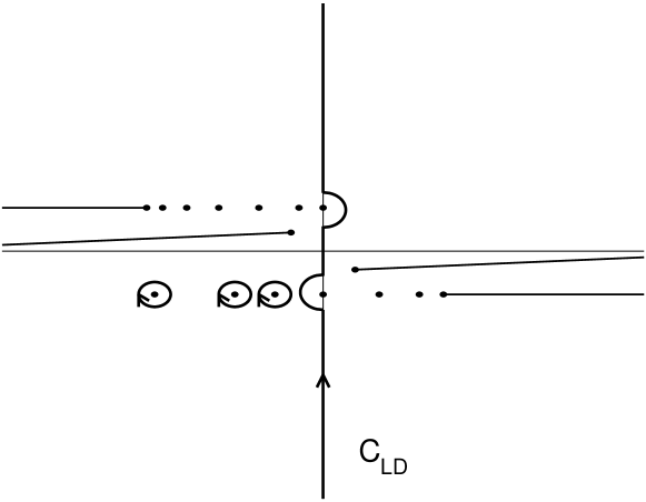
Figure 2: The poles and the branch cuts of the integrand for the direct part of the ladder contribution, and the integration contour $C_{\rm LD}$.

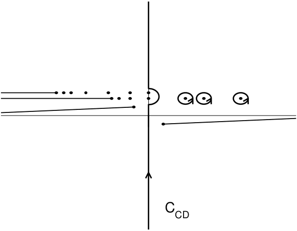
Figure 3: The poles and the branch cuts of the integrand for the direct part of the crossed contribution, and the integration contour $C_{\rm CD}$.

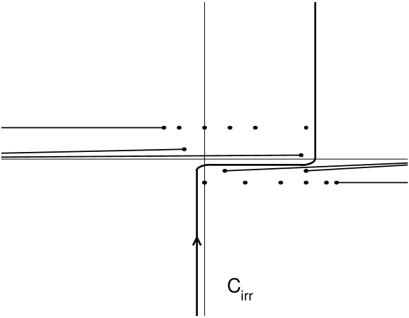
Figure 4: The poles and the branch cuts of the integrand for the exchange part of the ladder contribution, and the integration contour $C_{\rm irr}$.

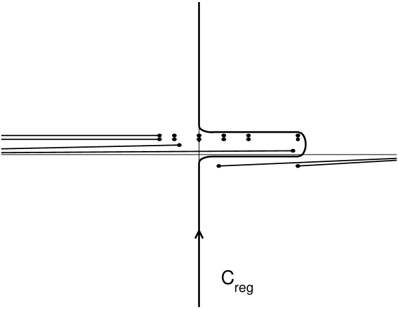
Figure 5: The poles and the branch cuts of the integrand for the exchange part of the crossed contribution, and the integration contour $C_{\rm reg}$.

The integration over the energy of the virtual photon $\omega$ in Eqs. (10)-(13) represents the most difficult part of the calculation. To avoid strong oscillations for large values of $\omega$, we performed the Wick rotation of the integration contour. Deforming the contour, one should take care about the poles and the branch cuts of the integrand. The analytic structure of the integrand for Eqs. (11)-(13) is shown in Figs. 2-5. These graphs are very similar to those for the $2s$- and $2p_{1/2}$-valence electrons in Ref. yerokhin01pra2p . The only difference is that now three Dirac energy levels occur which are more deeply bound than the valence state: $1s$, $2s$, and $2p_{1/2}$. The terms in Eqs. (11) and (13) containing these states and the valence state as intermediate were treated in a different way than the remainder, as is discussed below.

For the evaluation of the direct parts of the ladder and crossed contributions, we perform the Wick rotation of the integration contours separating the corresponding pole contributions, as shown in Figs. 2 and 3. In the direct part of the reducible contribution, we also perform a Wick rotation and then integrate by parts. This yields the following expression which can be evaluated directly,

$$\Delta E^{\rm 2el}_{\rm"red",dir} = \frac{1}{2}\left[F^{\rm lad}_{\rm dir}(\Delta_{vc},vc)\right]^{\prime}$$ (20)

$$- \frac{1}{\pi}\int_{0}^{\infty}d\omega\frac{\omega}{\Delta_{vc}^{2}+\omega^{2}}\frac{d}{d\omega}F^{\rm lad}_{\rm dir}(i\omega,vc)\,,$$

where $F^{\prime}(\Delta)=(dF/d\omega)_{\omega=\Delta}$.

Let us now turn to the exchange contribution. As one can see from Figs. 4 or 5, in this case the integration contour is squeezed between two branch cuts of the photon propagators on the interval $[0,\Delta_{vc}]$. Therefore, the standard Wick rotation of the contour is not possible. It is convenient to divide the contributions of Eqs. (11) and (13) into two parts. The first one accounts for the poles of the integrand on the interval $[0,\Delta_{vc}]$ and is referred to as the irregular part. The remainder is denoted as the regular part. This contribution does not possess any poles close to the squeezed part of the contour, which simplifies its numerical evaluation. However, it turns out as is the most time-consuming part of the calculation. One of the integration contours $C_{\rm reg}$ used for the evaluation of the regular part is depicted in Fig. 5.

The evaluation of the irregular part is less time consuming, but its structure is more difficult. In this case we need to take care of single and double poles of the integrand that are located close to the integration contour. The potential occurrences of one or two single poles and one double pole within the interval $[0,\Delta_{vc}]$ were treated by means of the following identities:

$$\int_{\omega_{1}}^{\omega_{2}}d\omega\frac{f(\omega)}{x_{0}-\omega\pm i0} = P\int_{\omega_{1}}^{\omega_{2}}d\omega\frac{f(\omega)}{x_{0}-\omega}\mp i\pi f(x_{0})\,,$$ (21)

$$\int_{\omega_{1}}^{\omega_{2}}d\omega\frac{f(\omega)}{(x_{0}-\omega\pm i0)^{2}} = \pm i\pi f^{\prime}(x_{0})+\frac{f(\omega_{2})}{x_{0}-\omega_{2}}$$ (22)

$$-\frac{f(\omega_{1})}{x_{0}-\omega_{1}}-P\int_{\omega_{1}}^{\omega_{2}}d\omega\frac{f^{\prime}(\omega)}{x_{0}-\omega}\,,$$

$$\int_{\omega_{1}}^{\omega_{2}}d\omega\frac{f(\omega)}{(x_{0}-\omega\pm i0)(x_{1}-\omega\pm i0)} = \frac{1}{x_{1}-x_{0}}\Biggl{[}P\int_{\omega_{1}}^{\omega_{2}}d\omega\frac{f(\omega)}{x_{0}-\omega}$$ (23)

$$-P\int_{\omega_{1}}^{\omega_{2}}d\omega\frac{f(\omega)}{x_{1}-\omega}\mp i\pi f(x_{0})\pm i\pi f(x_{1})\Biggr{]}\,,$$

where $P$ indicates the principal value of the integral. In Eq. (23) the choice of the sign before $i\pi f(x_{0})$ and $i\pi f(x_{1})$ is determined by the sign of the infinitesimal addition $\pm i0$ in the first and the second denominator, respectively. For the numerical evaluation of the irregular contribution we employed the integration contour $C_{\rm irr}$ shown in Fig. 4. It consists of 3 parts: $[-i\infty-\epsilon,-\epsilon]$, $[-\epsilon,\Delta_{vc}+\epsilon]$, and $[\Delta_{vc}+\epsilon,\Delta_{vc}+\epsilon+i\infty]$. A small positive constant $\epsilon$ was introduced in order to facilitate the numerical evaluation of the principal-value integrals.

After integration by parts, the exchange contribution of the reducible part can be written as

$$\Delta E^{\rm 2el}_{\rm"red",exch} = -\frac{1}{2}\Bigl{[}F^{\rm cr}_{\rm exch}(\Delta_{v}c,cc)+F^{\rm cr}_{\rm exch}(0,vv)\Bigr{]}^{\prime}$$ (24)

$$+\frac{1}{2\pi i}P\int_{-\infty}^{\infty}\frac{d\omega}{\omega}\frac{d}{d\omega}\Bigl{[}F^{\rm cr}_{\rm exch}(\Delta_{v}c+\omega,cc)$$

$$+F^{\rm cr}_{\rm exch}(\omega,vv)-2F^{\rm lad}_{\rm exch}(\omega,vc)\Bigr{]}\,.$$

It is again worth mentioning that the integral in Eq. (24) exists only if the sum of all 3 terms in the brackets is considered. For the each single term, the integral is infrared divergent.

IV Numerical results and discussion

The results of our calculations are presented in Table 1, where the direct, the exchange, and the three-electron contribution to the two-photon exchange correction of the valence $2p_{3/2}$ electron with the $(1s)^{2}$ shell are listed separately. The evaluation was performed within the Feynman gauge. We estimate the numerical uncertainty of our results to be less than $5\times 10^{-5}$ a.u. For bismuth, our results can be compared with the calculation by Sapirstein and Cheng sapirstein01 . They report $-6.529$ and $-6.670$ eV for the two-electron and the three-electron contribution, respectively. This agrees well with our corresponding results of $-6.5330$ and $-6.6698$ eV, respectively.

It is interesting to compare the results of the rigorous QED treatment with approximations evaluations based on relativistic many-body perturbation theory (MBPT). The difference between the QED and MBPT results can be conventionally regarded as a ”nontrivial” QED contribution. In order to deduce the two-photon exchange correction within the framework of MBPT, we should introduce the following changes in our basic formulas: all summations over intermediate states should be restricted to positive-energy states only, the calculation should be performed within Coulomb gauge, and the virtual-photon energy in the photon propagator should be set equal to zero. Within this approximation, all reducible parts vanish, and the integration over the energy of the virtual photon can be carried out employing Cauchy’s theorem. This yields zero for the crossed contribution, and finally we are left with the following expression for the total two-photon exchange correction within the MBPT approximation:

$$\Delta E_{\rm MBPT}^{\rm 3el} = \sum_{PQ}(-1)^{P+Q}\sum_{\varepsilon_{n}>0}\!^{\prime}\;\frac{I_{P2P3nQ3}(0)I_{P1nQ1Q2}(0)}{\varepsilon_{Q1}+\varepsilon_{Q2}-\varepsilon_{P1}-\varepsilon_{n}}\,,$$ (25)

$$\Delta E_{\rm MBPT}^{\rm 2el} = \sum_{\mu_{c}}\sum_{\varepsilon_{n_{1}}\varepsilon_{n_{2}}>0}\!\!\!^{\prime}\;\frac{\bigl{[}I_{cvn_{1}n_{2}}(0)-I_{vcn_{1}n_{2}}(0)\bigr{]}I_{n_{1}n_{2}cv}(0)}{\varepsilon_{c}+\varepsilon_{v}-\varepsilon_{n_{1}}-\varepsilon_{n_{2}}}\,,$$ (26)

where the photon propagators should be taken in the Coulomb gauge and the prime indicates that terms with vanishing denominator should be omitted. We mention that Eqs. (25) and (26) include the contribution due to the exchange by two Breit photons (the $B\times B$ term). Strictly speaking, this term is of higher order than the level of validity of the Breit approximation, and, therefore, it appears to be inconsistent to include it within the MBPT scheme.

In Table 2 and in Fig. 6 we compare the results of the rigorous QED treatment of the two-photon exchange correction to the $2p_{3/2}$-$2s$ splitting with the complete MBPT result [Eqs. (25) and (26)], and the MBPT result dropping the $B\times B$ term. A similar analysis for the $2p_{1/2}$-$2s$ splitting has been presented in our previous investigation yerokhin01pra2p . Our results show that in the case under consideration the nontrivial QED contribution is essentially larger than that for the $2p_{1/2}$-$2s$ transition. E.g., for uranium it yields $-0.011$ a.u., while the corresponding contribution to the $2p_{1/2}$-$2s$ splitting is two times smaller, of about $-0.006$ a.u. Moreover, we see that in our case the total correction changes its sign in the region between $Z=92$ and 100. As a result, the MBPT result becomes incorrect by more than 50% at very high values of $Z$. A further conclusion that can be drawn from our comparison is that for the $2p_{3/2}$-$2s$ splitting the $B\times B$ term is of the same sign and magnitude as the nontrivial QED contribution. Thus, its inclusion improves the agreement between the MBPT and the QED result. This situation is contrary to the one for the $2p_{1/2}$-$2s$ splitting, where the $B\times B$ term turns out to be of the same order of magnitude, but of different sign than the nontrivial QED contribution.

To summarize this investigation we presented a rigorous QED evaluation of the two-photon exchange correction for the $(1s)^{2}2p_{3/2}$ state of Li-like ions. Combining these results with the data for the $(1s)^{2}2s$ state from our previous study yerokhin01pra2p , we obtained the two-photon exchange correction for the $2p_{3/2}$-$2s$ splitting. This is an important step towards the final goal consisting in the evaluation of all two-electron second-order QED corrections to the $2p_{3/2}$-$2s$ transition energy for the Li isoelectronic sequence.

V Acknowledgments

This work was supported by the Russian Foundation for Basic Research (Grant No. 01-02-17248), by the Russian Ministry of Education (Grant No. E02-3.1-49), and by the program ”Russian Universities” (Grant No. UR.01.01.072). The work of A.N.A. and V.M.S. was supported by the joint grant of the Russian Ministry of Education and the Administration of Saint Petersburg (Grant No. PD02-1.2-79). V.A.Y. acknowledges the support of the foundation ”Dynasty” and the International Center for Fundamental Physics. The work of V.M.S. was supported by the Alexander von Humboldt Stiftung. We also acknowledge support from BMBF, DFG, DAAD, and GSI.

Table 1: Various contributions to the two-photon exchange correction for the $(1s)^{2}2p_{3/2}$ state of Li-like ions, in atomic units. The subscripts ”dir” and ”exch” label the direct and the exchange parts, respectively; the superscripts ”2el” and ”3el” refer to the two-electron and the three-electron contributions, respectively.

Z	$\Delta E^{\rm 2el}_{\rm dir}$	$\Delta E^{\rm 2el}_{\rm exch}$	$\Delta E^{\rm 3el}$	Total
20	0.03876	0.03902	$-$0.45509	$-$0.37731
28	$-$0.10511	0.03760	$-$0.31608	$-$0.38359
30	$-$0.12453	0.03715	$-$0.29807	$-$0.38545
32	$-$0.14058	0.03673	$-$0.28363	$-$0.38748
40	$-$0.18304	0.03465	$-$0.24844	$-$0.39683
47	$-$0.20486	0.03257	$-$0.23449	$-$0.40677
50	$-$0.21185	0.03156	$-$0.23126	$-$0.41156
54	$-$0.21978	0.03019	$-$0.22878	$-$0.41836
60	$-$0.22960	0.02795	$-$0.22801	$-$0.42967
66	$-$0.23789	0.02560	$-$0.22991	$-$0.44220
70	$-$0.24292	0.02392	$-$0.23233	$-$0.45133
74	$-$0.24772	0.02223	$-$0.23553	$-$0.46102
79	$-$0.25360	0.02001	$-$0.24047	$-$0.47406
80	$-$0.25477	0.01958	$-$0.24158	$-$0.47677
82	$-$0.25712	0.01867	$-$0.24390	$-$0.48236
83	$-$0.25831	0.01822	$-$0.24511	$-$0.48519
90	$-$0.26682	0.01499	$-$0.25454	$-$0.50636
92	$-$0.26936	0.01406	$-$0.25752	$-$0.51281
100	$-$0.28022	0.01030	$-$0.27070	$-$0.54061

Table 2: Comparison of the rigorous QED treatment of the two-photon exchange correction to the $2p_{3/2}$-$2s$ splitting in Li-like ions with the approximate MBPT treatment, in atomic units. ${B\times B}$ denotes the term corresponding to the exchange by two Breit photons.

Z	QED	MBPT	MBPT$-$(${B\times B}$)
20	$-$0.11912	$-$0.11917	$-$0.11920
28	$-$0.11778	$-$0.11784	$-$0.11794
30	$-$0.11731	$-$0.11741	$-$0.11754
32	$-$0.11681	$-$0.11693	$-$0.11709
40	$-$0.11414	$-$0.11449	$-$0.11483
47	$-$0.11078	$-$0.11147	$-$0.11205
50	$-$0.10897	$-$0.10985	$-$0.11056
54	$-$0.10606	$-$0.10732	$-$0.10825
60	$-$0.10064	$-$0.10258	$-$0.10391
66	$-$0.09355	$-$0.09640	$-$0.09824
70	$-$0.08756	$-$0.09125	$-$0.09352
74	$-$0.08044	$-$0.08508	$-$0.08786
79	$-$0.06960	$-$0.07562	$-$0.07915
80	$-$0.06711	$-$0.07345	$-$0.07715
82	$-$0.06183	$-$0.06879	$-$0.07286
83	$-$0.05898	$-$0.06630	$-$0.07056
90	$-$0.03514	$-$0.04509	$-$0.05096
92	$-$0.02676	$-$0.03759	$-$0.04401
100	0.01597	0.00138	$-$0.00781

Figure 1: Feynman diagrams for the two-photon exchange corrections.

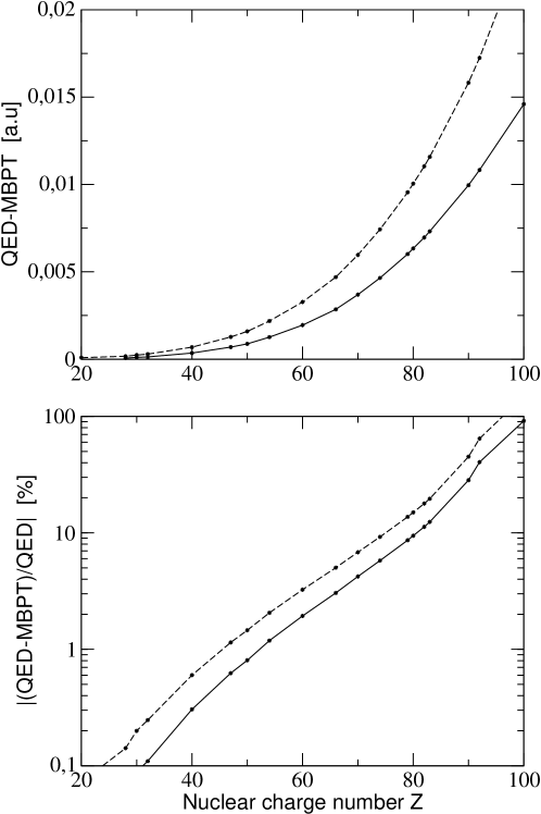
Figure 6: The difference of the QED result for the two-photon exchange correction to the $2p_{3/2}$-$2s$ transition and the corresponding MBPT results, with the $B\times B$ term included (solid line) and without this term (dashed line). The upper graph presents this difference in atomic units, and the lower one in units of per cent of the total QED contribution.

References

• (1) P.ย Beiersdorfer, A.ย L. Osterheld, J.ย H. Scofield, J.ย R. Crespo Lรณpez-Urrutia, and K.ย Widmann, Phys. Rev. Lett. 80, 3022 (1998).
• (2) P.ย Bosselmann, U.ย Staude, D.ย Horn, K.-H. Schartner, F.ย Folkmann, A.ย E. Livingston, and P.ย H. Mokler, Phys. Rev. A 59, 1874 (1999).
• (3) D.ย Feili, P.ย Bosselmann, K.-H. Schartner, F.ย Folkmann, A.ย E. Livingston, and P.ย H. Mokler, Phys. Rev. A 62, 022501 (2000).
• (4) C.ย Brandau, PhD thesis, University of GieรŸen, 2000.
• (5) A.ย N. Artemyev, T.ย Beier, G.ย Plunien, V.ย M. Shabaev, G.ย Soff, and V.ย A. Yerokhin, Phys. Rev. A 60, 45 (1999).
• (6) V.A. Yerokhin, A.N. Artemyev, T. Beier, G. Plunien, V.M. Shabaev, and G. Soff, Phys. Rev. A 60, 3522 (1999).
• (7) V.A. Yerokhin, A.N. Artemyev, V.M. Shabaev, M.M. Sysak, O.M. Zherebtsov, and G. Soff, Phys. Rev. Lett. 85, 4699 (2000).
• (8) V.ย A. Yerokhin, A.ย N. Artemyev, V.ย M. Shabaev, M.ย M. Sysak, O.ย M. Zherebtsov, and G.ย Soff, Phys. Rev. A 64, 032109 (2001).
• (9) J.ย Sapirstein and K.ย T. Cheng, Phys. Rev. A 64, 022502 (2001).
• (10) S.ย A. Blundell, P.ย J. Mohr, W.ย R. Johnson, and J.ย Sapirstein, Phys. Rev. A 48, 2615 (1993).
• (11) I.ย Lindgren, H.ย Persson, S.ย Salomonson, and L. Labzowsky, Phys. Rev. A 51, 1167 (1995).
• (12) P. J. Mohr and J. Sapirstein, Phys. Rev. A 62, 052501 (2000).
• (13) O. Yu. Andreev, L. N. Labzowsky, G. Plunien, and G. Soff, Phys. Rev. A 64, 042513 (2001).
• (14) O. Yu. Andreev, L. N. Labzowsky, G. Plunien, and G. Soff, Phys. Rev. A 67, 012503 (2003).
• (15) V.ย M. Shabaev, Izv. Vyssh. Uchebn. Zaved., Fiz. 33, 43 (1990), [Sov. Phys. J. 33, 660 (1990)].
• (16) V.ย M. Shabaev, Phys. Rev. A 50, 4521 (1994).
• (17) V.ย M. Shabaev, Physics Reports 356, 119 (2002).
• (18) V. M. Shabaev and I. G. Fokeeva, Phys. Rev. A 49, 4489 (1994).
• (19) M.ย M. Sysak, V.ย A. Erokhin, and V.ย M. Shabaev, Opt. Spektrosk. 92, 332 (2002), [Opt. Spectrosc. 92, 375 (2002)].
• (20) W.ย R. Johnson, S.ย A. Blundell, and J.ย Sapirstein, Phys. Rev. A 37, 307 (1988).