Asymptotic properties of self-energy coefficients

Abstract

We investigate the asymptotic properties of higher-order binding corrections to the one-loop self-energy of excited states in atomic hydrogen. We evaluate the historically problematic $A_{60}$ coefficient for all P states with principal quantum numbers $n\leq 7$ and D states with $n\leq 8$ and find that a satisfactory representation of the $n$-dependence of the coefficients requires a three-parameter fit. For the high-energy contribution to $A_{60}$, we find exact formulas. The results obtained are relevant for the interpretation of high-precision laser spectrocopic measurements.

Bound-state quantum electrodynamics (QED) occupies a unique position in theoretical physics in that it combines all conceptual intricacies of modern quantum field theories, augmented by the peculiarities of bound states, with the experimental possibilities of ultra-high resolution laser spectroscopy. Calculations in this area have a long history, and the current status of theoretical predictions is the result of continuous effort. The purpose of this Letter is twofold: first, to present improved evaluations of higher-order binding corrections to the bound-state self-energy for a large number of atomic states, including highly excited states with a principal quantum number as high as $n=8$, and second, to analyze the asymptotic dependence of the analytic results on the bound-state quantum numbers. Highly-excited states (e.g, with $n=4$ to $12$) are of particular importance for high-precision spectroscopy experiments in hydrogen (for a summary, see for instance (MoTa2000, , p. 371)).

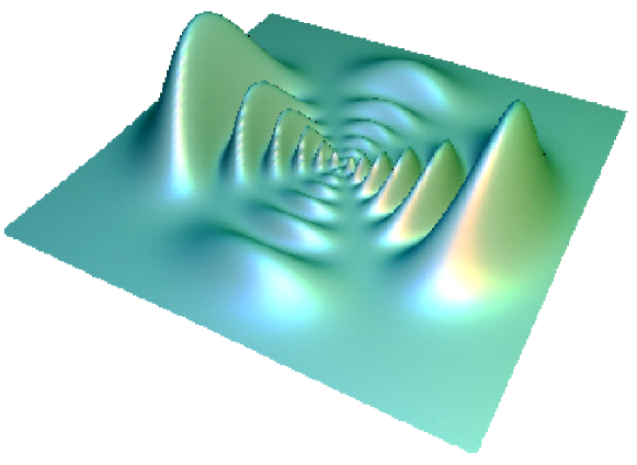
Figure 1: Plot of the radial probability density $r^{2}|\psi(r,\theta,\phi)|^{2}$ of the nonrelativistic 8D wave function (angular momentum projection $m=0$) in the plane of constant azimuth $\phi=0$. The calculation of the relativistic Bethe logarithm $A_{60}$ starts from this nonrelativistic wave function, with relativistic corrections being taken into account via generalized Foldy-Wouthuysen transformations JePa1996 ; JeSoMo1997 .

In the analytic calculations, we focus on a specific higher-order binding correction, known as the $A_{60}$ coefficient or “relativistic Bethe logarithm.” We write the (real part of the) one-loop self-energy shift of an electron in the field of a nucleus of charge number $Z$ as

$$\Delta E_{\rm SE}=\frac{\alpha}{\pi}\,\frac{(Z\alpha)^{4}}{n^{3}}\,F(nl_{j},Z\alpha)\,m\,c^{2}\,,$$ (1)

where $F(nl_{j},Z\alpha)$ is a dimensionless quantity. In this Letter, we use natural units with $\hbar=c=m=1$ and $e^{2}=4\pi\alpha$ ($m$ is the electron mass). The notation $nl_{j}$ is inspired by the usual spectroscopic nomenclature: $n$ is the level number, $j$ is the total angular momentum and $l$ is the orbital angular momentum.

The semi-analytic expansion of $F(nl_{j},Z\alpha)$ about $Z\alpha=0$ for a general atomic state with quantum numbers $n$, $l\geq 1$ and $j$ gives rise to the expression,

$$F(nl_{j},Z\alpha) = A_{40}(nl_{j})+(Z\alpha)^{2}\,\left[A_{61}(nl_{j})\,\ln(Z\alpha)^{-2}\right.$$ (2)

$$\left.+G_{\rm SE}(nl_{j},Z\alpha)\right]\qquad(l\geq 0)\,,$$

where $G_{\rm SE}(nl_{j},Z\alpha)\to{\rm constant}$ as $Z\alpha\to 0$. The limit as $Z\alpha\to 0$ of $G_{\rm SE}(nl_{j},Z\alpha)$ is referred to as the $A_{60}$ coefficient, i.e.

$$A_{60}(nl_{j})=\lim_{Z\alpha\to 0}G_{\rm SE}(nl_{j},Z\alpha)\,.$$ (3)

It is this coefficient which has proven to be by far the most difficult to evaluate ErYe1965a ; ErYe1965b ; Er1971 ; Sa1981 ; Pa1993 ; JeMoSo1999 . Furthermore, the complexity of the calculation increases sharply with increasing principal quantum number $n$, both due to the more involved structure of the bound-state wave function (see also Fig. 1), and due to the necessity of subtracting bound-state poles that lie infinitesimally close to the photon integration contour. The atomic states with the highest $n$ for which analytic results are available today are the 4P states JeSoMo1997 . In this Letter, we present analytic data for the $A_{60}$ coefficient of P states with $n\leq 7$ and all D states with $n\leq 8$. For a given $n$, the calculation is more involved for $n{\rm P}$ than for $n{\rm D}$, because there is one more term in the nonrelativistic radial $n{\rm P}$ wave function than in the corresponding $n{\rm D}$ wave function (when they are expressed as a function of the electron–nucleus distance). Essentially, the number of terms in the radial wave function determines the complexity of the calculation.

One of the most demanding specific calculations in the evaluation of $A_{60}$ is necessitated by a Bethe-logarithm type contribution given by the relativistic wave-function correction $F_{\delta\phi}$; this contribution is defined in Eqs. (43) and (53) of JePa1996 . For 7P and 8D states, we use up to 200,000 terms in intermediate steps in the evaluation of this correction. Because $A_{60}$ involves relativistic corrections to the coefficient $A_{40}$, which in turn is given mainly by the Bethe logarithm, it is natural to refer to the entire $A_{60}$ coefficient as a “relativistic Bethe logarithm.”

Table 1: $A_{60}$ coefficients for ${\rm P}_{1/2}$, ${\rm P}_{3/2}$, ${\rm D}_{3/2}$ and ${\rm D}_{5/2}$ states ($n=2,\dots,7$ for P states, and $n=3,\dots,8$ for D). The quantity ${\cal L}$ is implicitly defined in Eq. (Asymptotic properties of self-energy coefficients) and represents the low-energy contribution to $A_{60}$.

$n$	$A_{60}(n{\rm P}_{1/2})$	${\cal L}(n{\rm P}_{1/2})$	$A_{60}(n{\rm P}_{3/2})$	${\cal L}(n{\rm P}_{3/2})$
2	$-0.998~{}904~{}402(1)$	$-0.795~{}649~{}812(1)$	$-0.503~{}373~{}464(1)$	$-0.584~{}516~{}780(1)$
3	$-1.148~{}189~{}956(1)$	$-0.944~{}288~{}447(1)$	$-0.597~{}569~{}388(1)$	$-0.693~{}566~{}427(1)$
4	$-1.195~{}688~{}142(1)$	$-0.997~{}810~{}211(1)$	$-0.630~{}945~{}796(1)$	$-0.730~{}579~{}137(1)$
5	$-1.216~{}224~{}512(1)$	$-1.023~{}991~{}781(1)$	$-0.647~{}013~{}509(1)$	$-0.747~{}615~{}653(1)$
6	$-1.226~{}702~{}391(1)$	$-1.039~{}079~{}399(1)$	$-0.656~{}154~{}893(1)$	$-0.756~{}897~{}499(1)$
7	$-1.232~{}715~{}957(1)$	$-1.048~{}800~{}134(1)$	$-0.662~{}027~{}568(1)$	$-0.762~{}622~{}956(1)$
$n$	$A_{60}(n{\rm D}_{3/2})$	${\cal L}(n{\rm D}_{3/2})$	$A_{60}(n{\rm D}_{5/2})$	${\cal L}(n{\rm D}_{5/2})$
3	$0.005~{}551~{}575(1)$	$0.021~{}250~{}354(1)$	$0.027~{}609~{}989(1)$	$0.019~{}188~{}397(1)$
4	$0.005~{}585~{}985(1)$	$0.022~{}882~{}528(1)$	$0.031~{}411~{}862(1)$	$0.020~{}710~{}720(1)$
5	$0.006~{}152~{}175(1)$	$0.023~{}759~{}683(1)$	$0.033~{}077~{}571(1)$	$0.021~{}511~{}798(1)$
6	$0.006~{}749~{}745(1)$	$0.024~{}294~{}690(1)$	$0.033~{}908~{}493(1)$	$0.021~{}975~{}925(1)$
7	$0.007~{}277~{}403(1)$	$0.024~{}645~{}479(1)$	$0.034~{}355~{}926(1)$	$0.022~{}264~{}036(1)$
8	$0.007~{}723~{}850(1)$	$0.024~{}886~{}986(1)$	$0.034~{}607~{}492(1)$	$0.022~{}452~{}259(1)$

The “normal Bethe logarithm” $\ln k_{0}(nl)$ forms part of the coefficient $A_{40}$ for which a well-known general formula (see, e.g., Ref. (MoTa2000, , p. 468)) reads

$$A_{40}(nl_{j})=-\frac{1}{2\kappa\,(2l+1)}-\frac{4}{3}\,\ln k_{0}(nl)\,,$$ (4)

where $\kappa=2\,(l-j)\,(j+1/2)$. Formulas for $A_{61}$ valid for P and D states read as follows (see, e.g., Ref. (MoTa2000, , p. 468))

$$A_{61}(nP_{1/2}) = \frac{1}{45}\,\left(33-\frac{29}{n^{2}}\right)\,,$$ (5)

$$A_{61}(nP_{3/2}) = \frac{2}{45}\,\left(9-\frac{7}{n^{2}}\right)\,,$$ (6)

$$A_{61}(nl_{j}) = \frac{32\,\left(3-\frac{\displaystyle l\,(l+1)}{\displaystyle n^{2}}\right)}{3\prod\limits_{m=-1}^{3}(2\,l+m)}\quad(l\geq 2)\,.$$ (7)

Note that $A_{61}(nl_{j})\to{\rm constant}$ for $n\to\infty$ at constant $l$ and $j$. It is the purpose of this Letter to present new results for the $A_{60}$ coefficients. Details of our calculations will be presented in a forthcoming article lebigot2003c . It has been observed previously by Karshenboim Ka1997priv that the $n$-dependence of the $A_{60}(n{\rm P})$ coefficients can be fitted to a satisfactory accuracy by an $(n^{2}-1)/n^{2}$-type model, and a two-parameter fit has been employed for the $n$-dependence of the S-state coefficients $A_{60}(n{\rm S}_{1/2})$ Ka1997 . Our data for P states in Tab. 1 are roughly consistent with this $(n^{2}-1)/n^{2}$ model.

For the atomic states under investigation, the self-energy contribution due to hard virtual photons (high-energy part) obtained by the $\epsilon$ method Pa1993 ; JePa1996 ; JeSoMo1997 ; lebigot2003c is

$$F_{H}(nl_{j},Z\alpha)=-\frac{1}{2\kappa\,(2l+1)}$$

$$\quad{}+(Z\alpha)^{2}\,\left[{\cal K}-\frac{{\cal C}}{\epsilon}-A_{61}\,\ln(2\epsilon)+{\mathcal{O}}(\epsilon)\right]+\ldots$$

The ellipsis denotes higher-order terms, which are irrelevant for the current investigation. In Eq. (Asymptotic properties of self-energy coefficients), $\cal K$ and ${\cal C}$, as well as $A_{61}$, are state-dependent coefficients. For concrete evaluations of the high-energy part concerning specific atomic states, see (JePa1996, , Eqs. (18) and (19)) and (JeSoMo1997, , Eqs. (55)–(58)). The low-energy part assumes the form

$$F_{L}(nl_{j},Z\alpha)=-\frac{4}{3}\ln k_{0}(nl)$$

$${}+(Z\alpha)^{2}\,\left[{\cal L}+\frac{{\cal C}}{\epsilon}+A_{61}\,\ln\left(\frac{\epsilon}{(Z\alpha)^{2}}\right)+{\mathcal{O}}(\epsilon)\right]\,,$$

where we omit terms that are irrelevant at relative order $(Z\alpha)^{2}$ in the evaluation of $F(nl_{j},Z\alpha)$. A detailed explanation of the $\epsilon$ method will be given in lebigot2003c . The dependence on ${\cal C}$ cancels when the high- and low-energy parts are added. Specifically, we have

$$A_{60}={\cal K}-A_{61}\,\ln 2+{\cal L}\,.$$ (10)

Upon inspection of (Asymptotic properties of self-energy coefficients) and (Asymptotic properties of self-energy coefficients), we identify

$$A_{60,H}={\cal K}-A_{61}\,\ln 2$$ (11)

as the high-energy contribution to $A_{60}$, and $A_{60,L}={\cal L}$ as the low-energy contribution (see Figs. 2 and 3).

Table 2: Coefficients $L_{1}$, $L_{2}$ and $L_{3}$ that result from a least-squares fit of the $n$-dependence of our data for ${\cal L}$ in Tab. 1 (see also Figs. 2 and 3). The value of $L_{1}$ from this global fit should approximate the limit $\lim_{n\rightarrow\infty}{\cal L}(nl_{j})$ in Eq. (13), although it is not necessarily the best estimate.

state	$L_{1}$	$L_{2}$	$L_{3}$
${\rm P}_{1/2}$	$-1.082$	$0.0966$	$0.950$
${\rm P}_{3/2}$	$-0.775$	$-0.0232$	$0.811$
${\rm D}_{3/2}$	$0.0264$	$-0.00952$	$-0.0175$
${\rm D}_{5/2}$	$0.0235$	$-0.00568$	$-0.0220$

 

 

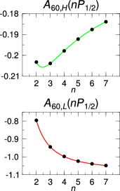
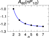
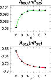
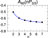
Figure 2: The plots show the dependence on the principal quantum number $n$ of the high- and low-energy part of the $A_{60}$ self-energy coefficient, as well as their sum ($A_{60}$). The curves for the high-energy contribution $A_{60,H}$ represent the exact results (5)–(7), (11), and (12), with $n$ being generalized to a continuous variable (only integer $n$ values have physical significance). The smooth curves for the low-energy parts $A_{60,L}={\cal L}$ result from a three-parameter fit of the data in Tab. 1 to the function in (13); the fit parameters are given in Tab. 2. The curves in the lower row represent the total result for $A_{60}=A_{60,H}+A_{60,L}$.

We obtain the following general formulas for ${\cal K}$:

$${\cal K}(n{\rm P}_{1/2}) = \frac{637}{1800}-\frac{1}{4n}-\frac{767}{5400\,n^{2}}\,,$$ (12a)

$${\cal K}(n{\rm P}_{3/2}) = \frac{2683}{7200}+\frac{1}{16n}-\frac{2147}{5400\,n^{2}}\,,$$ (12b)

$${\cal K}(n{\rm D}_{3/2}) = -\frac{157}{30240}-\frac{3}{80n}+\frac{3007}{37800\,n^{2}}\,,$$ (12c)

$${\cal K}(n{\rm D}_{5/2}) = \frac{379}{18900}+\frac{1}{60n}-\frac{1759}{18900\,n^{2}}\,.$$ (12d)

All of these formulas are consistent with a limit ${\cal K}\to{\rm constant}$ as $n\to\infty$ for constant $l$ and $j$. The $n$-dependence of the nonrelativistic ${\cal L}(nl_{j})$ contributions as listed in Tab. 1 can be approximated very well using a three-parameter fit inspired by the above structure found for the high-energy ${\cal K}$ contributions. We find

$${\cal L}(nl_{j})\approx L_{1}(l_{j})+\frac{L_{2}(l_{j})}{n}+\frac{L_{3}(l_{j})}{n^{2}}\,,$$ (13)

where $L_{1}$, $L_{2}$, and $L_{3}$ assume values as listed in Tab. 2 for the series of states under investigation. The $n$-dependence of the low-energy contributions ${\cal L}$ is smoother than the corresponding curves for the high-energy part (see Figs. 2 and 3). The excellent agreement of the fits with the numerical values of $A_{60,L}$, together with our exact results for the high-energy part as given by Eqs. (5)–(7), (11), and (12), could suggest a constant limit of $A_{60}(nl_{j})$ as $n\to\infty$ for constant $l$ and $j$.

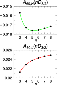
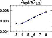
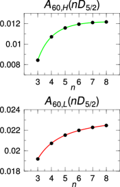
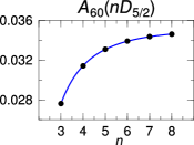
Figure 3: The analog of Fig. 2 for ${\rm D}_{3/2}$ and ${\rm D}_{5/2}$ states. The minimum in $A_{60,H}(n{\rm D}_{3/2})$ near $n=5$ is determined by the exact formulas (7) and (12c).

For Rydberg states with the highest $l$ possible for given $n$ (i.e., $l=\bar{l}=n-1$), our results are consistent with

$$\lim_{n\to\infty}A_{60}(n\bar{l}_{j})=0\text{ for }\bar{l}=n-1,\,j=n-1\pm 1/2\,,$$ (14)

which is plausible to suggest as a conjecture. The conjecture is indicated by the trend in the numbers ($j=\bar{l}-1/2$)

• $A_{60}(3{\rm D}_{3/2})=0.005~{}551~{}573(1)$,

• $A_{60}(4{\rm F}_{5/2})=0.002~{}326~{}988(1)$,

• $A_{60}(5{\rm G}_{7/2})=0.000~{}814~{}415(1)$,

as well as in the results ($j=\bar{l}+1/2$)

• $A_{60}(3{\rm D}_{5/2})=0.027~{}609~{}989(1)$,

• $A_{60}(4{\rm F}_{7/2})=0.007~{}074~{}961(1)$,

• $A_{60}(5{\rm G}_{9/2})=0.002~{}412~{}929(1)$.

The magnitude of $A_{60}(n\bar{l}_{j})$ appears to decrease faster than $1/n$. In general, relativistic corrections acquire at least one more inverse power of $n$ when $n=l+1$, $j=n-1\pm 1/2$, and $n$ large, than S or P states of the same $n$. This can for example be seen in the relativistic correction of order $(Z\alpha)^{4}$ to the Schrödinger-Coulomb electron energy [Eq. (2-87) of ItZu1980 ],

$$E_{nj} = m-\frac{(Z\alpha)^{2}\,m}{2n^{2}}$$

$${}-\frac{(Z\alpha)^{4}\,m}{n^{3}}\,\left[\frac{1}{2j+1}+\frac{3}{8\,n}\right]+{{\mathcal{O}}}[(Z\alpha)^{6}].$$

For $j=n-1\pm 1/2$, this relativistic term acquires an additional inverse power of $n$. Our results suggest that analogous statements hold for radiative corrections given by relativistic Bethe logarithms.

We have presented results of a calculation of higher-order binding corrections to the one-loop self-energy for highly excited hydrogenic atomic levels (see Tab. 1). Calculational difficulties induced by the more complex analytic structure of the wave functions have been a severe obstacle for evaluations of relativistic Bethe logarithms at high $n$, and no prior results are available for $A_{60}$ for any state with $n>4$ (see Ref. JeSoMo1997 ). Intermediate expressions contained up to 200,000 terms; without a computer, this work would have been impractical. Our calculation is split into a high- and a low-energy part. We find that the dependence of the low-energy contribution to $A_{60}$ on the principal quantum number of the atomic state under investigation can in many cases be represented accurately using a three-parameter fit [see Eq. (13) and the data in Tab. 2]. As suggested by the exact formulas for the high-energy part given in Eq. (12) and the curves in Figs. 2 and 3, a fit with less than three parameters cannot be assumed to lead to a satisfactory representation of $A_{60}$. Our final results for $A_{60}$ are given in Tab. 1. We establish that the magnitude of $A_{60}$ decreases rapidly for Rydberg states with the highest possible angular momentum for each principal quantum number. Our calculations improve the knowledge of the self-energy of an electron bound to a nucleus [see Eqs. (1)–(3) and Tab. 1]. They are motivated by the dramatically increasing precision of laser spectrocopy BeEtAl1997 ; ScEtAl1999 ; ReEtAl2000 ; NiEtAl2000 , which is rapidly approaching the $1~{}{\rm Hz}$ level of accuracy. For the determination of fundamental constants from high-resolution spectroscopy, frequency measurements of at least two different transitions have to be performed. Highly excited, slowly decaying D states are attractive because they can be excited out of S states via two-photon resonance BeEtAl1997 ; MoTa2000 .

The authors would like to acknowledge helpful discussions with K. Pachucki, S. Jentschura and J. Sims. U.D.J. acknowledges support from the Deutscher Akademischer Austauschdienst (DAAD). E.O.L. acknowledges support from a Lavoisier fellowship of the French Ministry of Foreign Affairs, support by NIST, and a grant of computer time at the CINES (Montpellier, France). G.S. acknowledges support from BMBF, DFG and from GSI. The Kastler Brossel laboratory is Unité Mixte de Recherche 8552 of the CNRS.

References

- (1) P. J. Mohr and B. N. Taylor, Rev. Mod. Phys. 72, 351 (2000).
- (2) G. W. Erickson and D. R. Yennie, Ann. Phys. (N. Y.) 35, 271 (1965).
- (3) G. W. Erickson and D. R. Yennie, Ann. Phys. (N. Y.) 35, 447 (1965).
- (4) G. W. Erickson, Phys. Rev. Lett. 27, 780 (1971).
- (5) J. Sapirstein, Phys. Rev. Lett. 47, 1723 (1981).
- (6) K. Pachucki, Ann. Phys. (N. Y.) 226, 1 (1993).
- (7) U. D. Jentschura, P. J. Mohr, and G. Soff, Phys. Rev. Lett. 82, 53 (1999).
- (8) U. Jentschura and K. Pachucki, Phys. Rev. A 54, 1853 (1996).
- (9) U. D. Jentschura, G. Soff, and P. J. Mohr, Phys. Rev. A 56, 1739 (1997).
- (10) E.-O. Le Bigot, U. D. Jentschura, P. J. Mohr, P. Indelicato, and G. Soff, The Bound-Electron Perturbative Self Energy of non-S States, submitted (2003).
- (11) S. G. Karshenboim, private communication (1997).
- (12) S. G. Karshenboim, Z. Phys. D 39, 109 (1997).
- (13) C. Itzykson and J. B. Zuber, Quantum Field Theory (McGraw-Hill, New York, NY, 1980).
- (14) B. de Beauvoir, F. Nez, L. Julien, B. Cagnac, F. Biraben, D. Touahri, L. Hilico, O. Acef, A. Clairon, and J. J. Zondy, Phys. Rev. Lett. 78, 440 (1997).
- (15) C. Schwob, L. Jozefowski, B. de Beauvoir, L. Hilico, F. Nez, L. Julien, F. Biraben, O. Acef, A. Clairon, Phys. Rev. Lett. 82, 4960 (1999).
- (16) J. Reichert, M. Niering, R. Holzwarth, M. Weitz, T. Udem, and T. W. Hänsch, Phys. Rev. Lett. 84, 3232 (2000).
- (17) M. Niering, R. Holzwarth, J. Reichert, P. Pokasov, T. Udem, M. Weitz, T. W. Hänsch, P. Lemonde, G. Santarelli, M. Abgrall, P. Laurent, C. Salomon, and A. Clairon, Phys. Rev. Lett. 84, 5496 (2000).