Noise sensitivity of sub- and supercritically bifurcating patterns with group velocities close to the convective-absolute instability

Abstract

The influence of small additive noise on structure formation near a forwards and near an inverted bifurcation as described by a cubic and quintic Ginzburg Landau amplitude equation, respectively, is studied numerically for group velocities in the vicinity of the convective-absolute instability where the deterministic front dynamics would empty the system.

I Introduction

The formation of macroscopic structures CH93 in systems that are driven out of thermal equilibrium by an externally imposed generalized stress are usually investigated by deterministic field equations. However, under specific circumstances the influence of external deterministic or stochastic perturbations and of internal thermal noise on the pattern formation process should be taken into account to achieve a more realistic and quantitative description of experiments. One prominent example are the so-called noise sustained structures D85 ; BAC ; Steinberg ; MLK92 ; SR92 ; LR93 ; SBH94 ; Deissler94 ; NWS96 ; LS97 ; T97 ; SCMW97 ; CWS99 in the convectively unstable parameter regime BersBriggs ; Huerre in, e.g., the Taylor-Couette BAC ; Steinberg ; LR93 ; SBH94 ; Deissler94 , the Rayleigh-Bénard MLK92 ; SR92 ; T97 system, or nonlinear optics SCMW97 . Further examples are certain open-flow instabilities , e.g., in wakes and jets that are reviewed in Huerre .

The noise sustained structures D85 ; BAC ; Steinberg ; MLK92 ; SR92 ; LR93 ; SBH94 ; Deissler94 ; NWS96 ; LS97 ; T97 ; SCMW97 ; CWS99 arise when an externally imposed through-flow or an internally generated group velocity $v$ is large enough to ”blow” the pattern out of the system according to the deterministic field equations. In this driving regime one observes in experiments BAC ; Steinberg ; SR92 ; T97 ; SCMW97 structures that are sustained by sources that generate perturbations in the band of modes that are amplified according to the supercritical deterministic growth dynamics in downstream direction sufficiently far away from the inlet.

The criterion BersBriggs ; Huerre at which $v$ the pattern is blown out of the system under deterministic laws which gave the threshold for the appearance of the noise sustained, supercritically bifurcating patterns in the above described experiments is a linear one. It was nonlinearly extended by Chomaz Chomaz92 to the question of the propagation direction of nonlinear deterministic fronts in infinite systems that connect the unstructured state to the finite-amplitude structured one.

Here we study and compare the noise sensitivity of pattern forming systems in which the above described fronts are linear or nonlinear ones. To that end we investigate the cubic Ginzburg-Landau amplitude equation (GLE) for a supercritical forwards bifurcation and the quintic GLE for a subcritical inverted bifurcation, respectively, in one spatial dimension.

We solve the GLE with additive stochastic forcing numerically. Our systems are finite but sufficiently long to allow the establishment of a statistically stationary large-amplitude bulk part – provided the latter is possible with the boundary condition of vanishing amplitude at the ends. We focus our attention to parameters in the vicinity of the convective-absolute threshold at which the fronts of the deterministic GLE cease to propagate. And we investigate in particular the statistical dynamics of phase and amplitude fluctuations in the front region.

II SYSTEM

We consider the stochastic, 1D Ginzburg-Landau equation

$$(\partial_{t}+v\partial_{x})A\;=\;(\mu+\partial_{x}^{2}+g_{3}|A|^{2}+g_{5}|A|^{4})A+\sigma\eta$$ (1)

for the complex amplitude

$$A\;=\;\Re A+{\rm i}\,\Im A\;=\;Re^{{\rm i}\,\Phi}$$ (2)

depending on $x,t$. Here $\Re(\Im)$ denotes the real (imaginary) part and $R=|A|$ is the modulus and $\Phi$ the phase of $A$. The coefficients in (1) are taken as real for simplicity. We checked however that taking into account the (small) imaginary parts, that appear e.g. in the case of transverse Rayleigh-Bénard convection rolls propagating downstream in a small externally imposed lateral through-flow MLK92 or in the case of downstream propagating Taylor vortices BAC ; RLM93 does not change the major findings presented in this paper significantly. We consider the group- or mean flow velocity $v\geq 0$ in positive $x$-direction and the linear growth rate $\mu$ of $A$ as control parameters.

We investigate two fixed combinations of the nonlinear coefficients ($g_{3},g_{5}$) that we refer to in this paper as follows

$$g_{3}\;=\;-1\;,\;g_{5}\;=\;0\; :$$ cubic GLE (3a)

$$g_{3}\;=\;1\;,\;g_{5}\;=\;-1\; : \quad\mbox{quintic GLE}\,.$$ (3b)

The quantity $\sigma$ in (1) measures the real strength of the complex stochastic force

$$\eta(x,t)\;=\;\Re\eta(x,t)+{\rm i}\,\Im\eta(x,t)$$ (4)

with statistically independent real and imaginary parts $\Re\eta$ and $\Im\eta$, respectively. Both are Gaussian distributed with zero mean and $\delta$-correlated such that

$$<\eta(x_{1},t_{1})[\eta(x_{2},t_{2})]^{*}>\;=\;2\delta(x_{1}-x_{2})\delta(t_{1}-t_{2})\;.$$ (5)

II.1 Unforced homogeneous solution

We are interested in the effect of small additive noise on the spatio-temporal structure formation in large but finite or semiinfinite systems. Nevertheless it is useful to briefly recall first the properties of the most simple solutions of the unforced GLE in an infinite system. This shows what one might expect to see in the bulk of a very large system far away from the boundaries — ignoring for the moment questions related to boundary induced pattern selection processes.

The GLE (1) shows for $\sigma$=0 a continuous family of traveling wave (TW) solutions

$$A(x,t)=Re^{iq(x-vt)}$$ (6)

with constant wave number $q$, frequency $\Omega=-qv$, and modulus $R$ given by

$$\mu-q^{2}+g_{3}R^{2}+g_{5}R^{4}=0\,.$$ (7)

This TW solution family bifurcates at the marginal stability curve, $\mu=q^{2}$, of the $A$=0 solution out of the latter while the former becomes unstable there. The critical values are $\mu_{c}=q_{c}=\Omega_{c}$=0. The bifurcation is nonhysteretic and forwards in the cubic case

$$R^{2}=\mu-q^{2}$$ (8)

and hysteretic, backwards in the quintic case

$$R^{2}=\frac{1}{2}\pm\sqrt{\mu-q^{2}+\frac{1}{4}}\,.$$ (9)

Here the lower sign refers to the lower unstable TW solution branch that exists for $-\frac{1}{4}\leq\mu-q^{2}\leq 0$. The upper TW solution branch identified by the + sign in Eq. (9) exists beyond the saddle-node bifurcation value $\mu=q^{2}-\frac{1}{4}$. These TW solutions are stable for wave numbers outside the Eckhaus unstable band BD92 .

II.2 Convective-absolute instability

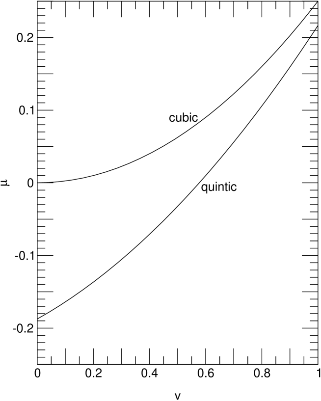
Figure 1: Convective-absolute instability boundaries (12) for the unforced cubic and quintic GLE, respectively. For parameters below the respective curve front propagation is such that in the absence of noise the $A$=0 state invades the $A\neq$0 state. In the absolutely unstable parameter regime above the respective curve the $A$=0 state recedes and the $A\neq$0 state expands (as long as the front is not hindered by a boundary).

The noise susceptibility of the pattern formation process described by the GLE (1) changes significantly D85 ; Huerre when crossing the parameter combination of $\mu,v$ shown in Fig. 1 for the so called convective-absolute instability BersBriggs . This combination

$$\mu_{c-a}=\left\{\begin{array}[]{ll}\frac{1}{4}v^{2}&\mbox{cubic GLE}\\ \frac{3}{16}\left(v^{2}+\frac{2}{\sqrt{3}}v-1\right)&\mbox{quintic GLE}\end{array}\right.$$ (12)

is marked by the front solution of the deterministic GLE with $\sigma=0$ undergoing a reversal of the front propagating direction in an infinite system. Consider a front that connects the basic state $A=0$ being realized at $x\to-\infty$ to a homogeneous solution with $A\neq 0$ at $x\to\infty$. For parameter values below (above) the respective curves in Fig. 1 this front moves to the right (left). Thus the basic state $A=0$ (the homogeneous solution $A\neq 0$) expands to the right (left). The region below (above) the respective curves in Fig. 1 where the basic state $A=0$ (the homogeneous state $A\neq 0$) invades the whole system is called the convectively (absolutely) unstable region of the $A=0$ solution D85 ; Huerre . Thus, the boundary (12) is also called the convective-absolute instability boundary.

For the cubic GLE the boundary $\mu_{c-a}=v^{2}/4$ results from a linear analysis D85 . For the backwards bifurcating solution arising in the quintic GLE the respective front that reverts its propagation direction is a nonlinear one SH92 . Note that in the latter case the convective-absolute instability boundary Chomaz92 connects for $v\to 0$ to the so-called Maxwell point $\mu_{c-a}=\mu_{M}=-3/16$: For this value the minima of the potential $V(A)=-\frac{\mu}{2}A^{2}-\frac{1}{4}A^{4}+\frac{1}{6}A^{6}$ have equal height $V=0$.

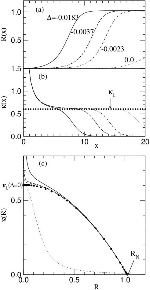
Figure 2: Deformation of the front solution $R(x)$ (a) of the deterministic quintic GLE by the boundary condition $A(x=0,t)=0$ in the absolutely unstable regime for $\mu=0.05$ and $v=(1+\Delta)v_{c-a}$ as indicated. The spatial growth rate $\kappa(x)=\partial_{x}ln{R(x)}$ (b) deviates from a freely propagating front with wave number $q=0$ that would show SH92 $\kappa_{L}=\frac{v}{2}+\sqrt{\frac{v^{2}}{4}-\mu}$ [thick dots in (b)] in the small-amplitude ”linear” part of the front. (c) shows $\kappa$ versus $R$ in comparison with the prediction SH92 $\kappa=\frac{1}{\sqrt{3}}\left(R_{N}^{2}-R^{2}\right)$ for a stationary front in an infinite system at $\Delta=0,\,\mu=0.05$ for which $R_{N}^{2}$=1.048. Thin dotted curves in (a)-(c) refer to a numerically obtained solution for $\Delta=0$ at time $5\cdot 10^{4}$ which is not yet stationary. Here the profile is still moving to the right and in the absence of numerical ”noise” we would expect this transient to approach the $R\equiv 0$ basic state [c.f. also Fig. (c)].

The boundary condition $A(x=0,t)=0$ that we apply in our simulations stops any front propagating to the left and it changes, i.e., it deforms the front profile when the front is sufficiently close to the boundary at $x=0$. This can be seen in Fig. 2 for the example of the deterministic quintic GLE. There the lines show the modulus profile $R$ and the spatial growth rate $\kappa=R^{\prime}/R$ versus $x$ together with $\kappa$ versus $R$ obtained numerically for several parameter values above the convective-absolute instability boundary. To facilitate comparison of different cases we introduce the reduced horizontal ”distance”

$$\Delta\;=\;\frac{v}{v_{c-a}}-1$$ (13)

from the boundaries shown in Fig. 1. Here

$$v_{c-a}(\mu)\;=\;\left\{\begin{array}[]{ll}2\sqrt{\mu}&\mbox{cubic GLE}\\ \sqrt{\frac{4}{3}\left(1+4\mu\right)}-\sqrt{\frac{1}{3}}&\mbox{quintic GLE}\end{array}\right.$$ (16)

denotes the convective-absolute instability boundary (12).

The results that we present here were obtained for $\mu>0$, i.e., in a situation where the basic state $A=0$ is unstable. For the backwards bifurcation in the quintic GLE with negative growth rates $-\frac{3}{16}<\mu<0$ for which the above cited potential has a minimum at $A=0$ the situation is more complicated CWS99 : Not only does the establishment of the final front connecting the inlet condition $A=0$ with a statistically stationary saturated bulk with $|A|={\cal O}(1)$ depend sensitively on the initial condition [say, $A(x,t=0)=0$ versus $|A|={\cal O}(1)$] in the absolutely unstable regime, $\Delta<0$. But more importantly, in the convectively unstable regime, $\Delta>0$, we found that small noise does not seem to be able to generate with the boundary condition $A(x=0)=0$ a noise sustained finite-amplitude structure with $\langle|A|^{2}\rangle$ of order one when $\mu<0$: The deterministic front dynamics drives the large-amplitude part downstream and eventually any finite system is filled only with small-amplitude fluctuations of $A$ around the stable fixed point $A=0$ of the unforced system.

II.3 Noise strength

For the quintic GLE we choose the noise strength $\sigma=10^{-3}$. The noise intensity $\sigma^{2}$ should be compared with the minimum of the potential

$$V(A)=-\frac{\mu}{2}A^{2}-g_{3}\frac{1}{4}A^{4}-g_{5}\frac{1}{6}A^{6}\,.$$ (17)

For our quintic case ($g_{3}=1,g_{5}=-1$) the minimum at $A^{2}=R_{N}^{2}=\frac{1}{2}+\sqrt{\frac{1}{4}+\mu}$ is $V(R_{N})=-\frac{1}{24}[1+6\mu+(1+4\mu)^{3/2}]$. Thus, the noise ”temperature” $\sigma^{2}$ measured in units of $V(R_{N})$ is $\sigma^{2}/|V(R_{N})|=9.2\,10^{-6}$ for the control parameter $\mu=0.05$ that we have used in most of our calculations.

A rough estimate for an equivalent noise strength for the cubic GLE would be to demand that the reduced noise ”temperature” $\sigma^{2}/V(R_{N})$ is in both cases the same. This would require for the cubic GLE at a common $\mu$ of, say, 0.05 that $\sigma$ is by about a factor of 13 smaller than for the quintic GLE.

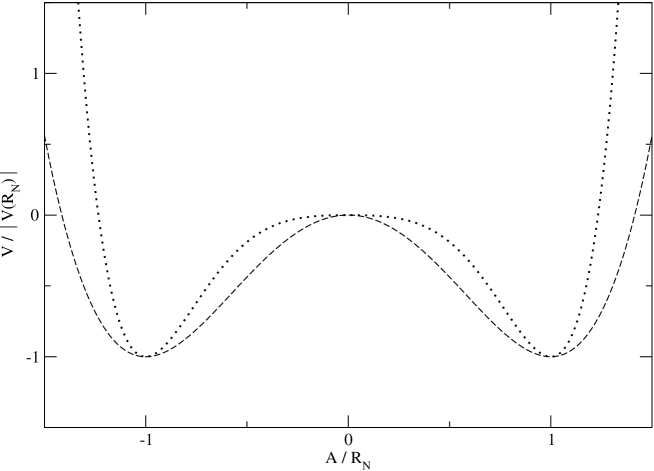
Figure 3: Reduced potentials V (17) corresponding to the real cubic (dashed line) and quintic (dotted line) GLE. For the cubic case the plot is independent of $\mu,g_{3}$. For the quintic case it depends on the combination $\tilde{\mu}=-g_{5}\mu/g_{3}^{2}$. Here $\tilde{\mu}=0.05$.

However, basing the comparison on the requirement that $\sigma^{2}/V(R_{N})$ is the same for the cubic and quintic case one has to keep in mind that the curvatures of $V$ around the states $A=0$ and $A=R_{N}$ which are connected by the fronts remain different – cf. Fig. 3. Since these curvatures around $A=0$ ($A=R_{N}$) measure the growth (decay) rates of fluctuations around the respective states it is useful to compare their ratios via a kind of Ginzburg number $G=|V^{{}^{\prime\prime}}(0)|/V^{{}^{\prime\prime}}(R_{N})$. One has $G_{cubic}=1/2$ independent of $\mu$ and $g_{3}$ while $G_{quintic}=\tilde{\mu}\left[1+4\tilde{\mu}+\sqrt{1+4\tilde{\mu}}\right]^{-1}$ with $\tilde{\mu}=-g_{5}\mu/g_{3}^{2}$. Thus for $\mu=0.05$ and $g_{3}=1,g_{5}=-1$ one has $G_{cubic}\simeq 23~{}G_{quintic}$. This largely explains the stronger noise sensitivity of the cubic GLE for our parameters. In view of it we investigated the whole range of $\sigma$ between $10^{-9}$ and $10^{-2}$ for the cubic GLE.

The cubic GLE with additional (but very small) complex coefficients has previously been investigated, e.g., for noise strengths of about $\sigma=1.9\cdot 10^{-6}$ in our units of eqs. (1-5). The corresponding noise ”temperature” $\sigma^{2}/V(R_{N})$ is about $10^{-8}$ for a typical value of, say, $\mu=0.035$ BAC . This noise was found to fit the experimental results on the noise sustained traveling Taylor vortices under statistically stationary fronts in the convectively unstable regime of open Taylor-Couette systems with axial through-flow BAC .

II.4 Numerical methods

Equation (1) was solved numerically with a forward-time, centered-space method Pre94 subject to the boundary conditions

$$A(x=0,t)\;=\;0\;=\;A(x=L,t)$$ (18)

on the complex amplitude. System sizes $L$ were chosen to be sufficiently large to allow for the establishment of a saturated bulk amplitude. Typically, a spatial step $dx=0.4$ was used with a time step of $dt=0.072$. Calculations were performed for sequences of the paramater $v$ at several values of the control parameter $\mu$. Most of them were done at $\mu=0.05$. The noise source $\eta$ was realized by Gaussian distributed random numbers of unit variance that were divided by $\sqrt{dtdx}$ to ensure independence of the correlation functions of the discretization. A test of different pseudo random number generators, namely, L’Ecuyer’s method with Bays-Durham shuffle Pre94 , ran3 Pre94 , and the R250 shift-register random number generator R250 gave similar results.

After the simulations were started, a sufficiently long time depending on the parameters, e.g., on the closeness to the convective-absolute threshold had to be waited until the system relaxed into a statistically stationary state with time independent averages. Thereafter time averages were evaluated over several consecutive time intervals and finally averaged. Within the forward-time integration method $A(x,t)$ remains uncorrelated with $\eta(x^{\prime},t)$ at the same time, $<f(\eta)g(A)>\;=\;<f(\eta)><g(A)>$, so that, e.g., $<A\eta>\;=\;0$ as well as $<q\eta>\;=\;0$. But $<\Omega\eta>\;\neq\;0$. Here the frequency $\Omega$ (wave number $q$) is defined as a forward-time (centered-space) difference of the phase (20).

III Results

The influence of additive noise on the pattern formation process described by the GLE (1) is described in this section.

III.1 Growth length $\ell$

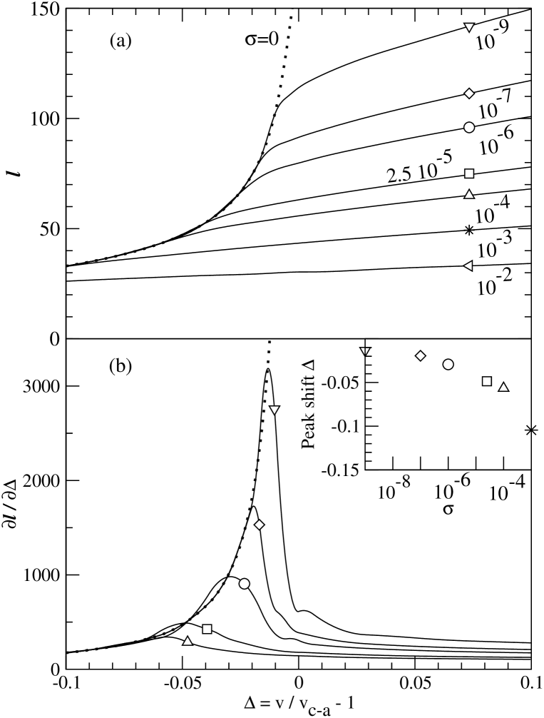
Figure 4: Growth length $\ell$ (a) and its derivative $\partial\ell/\partial\Delta$ (b) versus $\Delta$ near the convective-absolute threshold for the cubic GLE at $\mu=0.05$ for various noise strengths $\sigma$. Inset in (b) shows the variation of the peak of $\partial\ell/\partial\Delta$ with $\sigma$.

In Fig. 4 we show how the growth length $\ell$ of the downstream pattern occurring in the forced cubic GLE varies with noise strength $\sigma$. Here $\ell$ is defined by the distance from $x=0$ at which the root-mean square $\sqrt{<|A|^{2}>}$ of the fluctuating complex amplitude $A$ reaches half its bulk value. In the absence of noise $\ell$ diverges at the convective-absolute threshold $v=v_{c-a}$ since there the deterministic pattern is blown out of the system.

For finite $\sigma$ the solution with finite $A$ is noise-sustained in the convectively unstable regime $\Delta>0$ D85 . In this regime $\ell$ is far from the convective-absolute threshold well described by the relation $\ell\sim-(1+\sqrt{2\Delta})\ln{\sigma}$ following from a quasilinear analysis of the cubic GLE LS97 presented here in an appendix. However in the vicinity of the threshold $\Delta\,=\,0$ the growth length $\ell$ obtained from the nonlinear GLE shows a characteristic crossover to the behavior at $\Delta<0$.

The noise influences also in this absolutely unstable regime, $\Delta<0$, the finite amplitude solution at least close to threshold: The curves $\ell(\Delta,\sigma)$ in Fig. 4(a) break away from the dotted $\ell(\Delta,\sigma=0)$ reference growth length curve at negative $\Delta$ values that decrease with increasing $\sigma$, i.e., further and further away from the convective-absolute threshold. The associated inflection points can be most easily identified by the maxima in $\partial\ell(\Delta,\sigma)/\partial\Delta$ shown in Fig. 4(b). These peak positions of $\partial\ell/\partial\Delta$ vary with $\sigma$ as shown in the inset of Fig. 4(b). So the growth length shows for the cubic GLE a definite noise sensitivity also in the absolutely unstable regime.

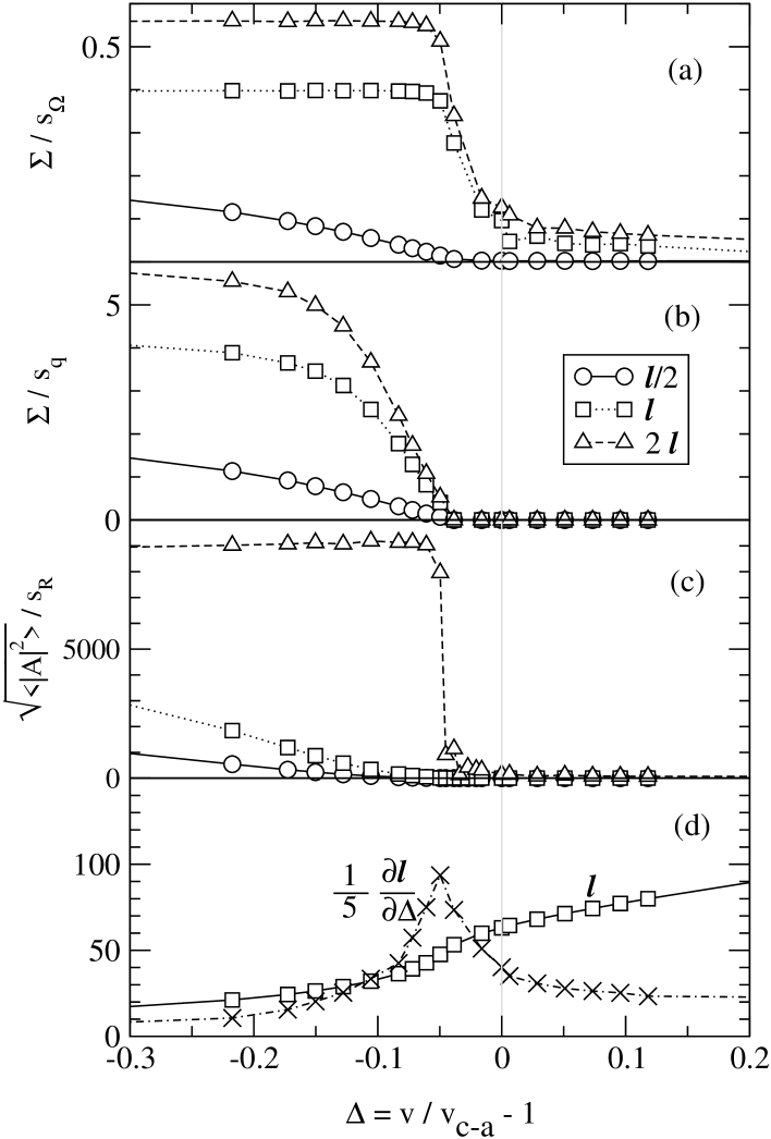
Figure 5: Inverse of the standard deviations of frequency $s_{\Omega}$ (a), wave number $s_{q}$ (b), and amplitude modulus $s_{R}$ (c) for the stochastic cubic GLE. Results are reduced by $\Sigma$ (26) or $\sqrt{<|A|^{2}>}$, respectively, and plotted as functions of $\Delta$ for three downstream locations $x=\ell/2$, $\ell$, and $2\ell$. (d) shows the growth length $\ell$ of $\sqrt{<|A|^{2}>}$ together with its derivative $\partial\ell/\partial\Delta$. Piecewise straight lines are guides to the eye. Parameters are $\mu=0.05$ and $\sigma=2.5\cdot 10^{-5}$.

This sensitivity is significantly smaller in the quintic GLE. This can be seen by comparing the behavior of the growth length with the fluctuations of the modulus $R=|A|$, of the frequency, and of the wave-number (cf, Sec. III.2). To that end we show in Figs. 5 and  6 $\ell$ and $\partial\ell/\partial\Delta$ together with the inverse of the standard deviations of the modulus

$$s_{R}=\sqrt{<R^{2}>-<R>^{2}}\,,$$ (19)

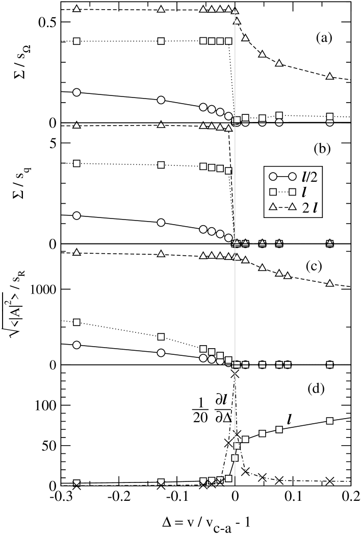
Figure 6: Inverse of the standard deviations of frequency $s_{\Omega}$ (a), wave number $s_{q}$ (b), and amplitude modulus $s_{R}$ (c) for the stochastic quintic GLE. Results are reduced by $\Sigma$ (26) or $\sqrt{<|A|^{2}>}$, respectively, and plotted as functions of $\Delta$ for three downstream locations $x=\ell/2$, $\ell$, and $2\ell$. (d) shows the growth length $\ell$ of $\sqrt{<|A|^{2}>}$ together with its derivative $\partial\ell/\partial\Delta$. Piecewise straight lines are guides to the eye. Parameters are $\mu=0.05$ and $\sigma=10^{-3}$.

of the frequency $s_{\Omega}$ (29), and of the wave-number $s_{q}$ (29) at $\mu$=0.05 as functions of $\Delta$ for the cubic and quintic GLE, respectively. The noise strengths $\sigma=2.5\cdot 10^{-5}$ and $10^{-3}$, respectively, used for these figures are roughly equivalent based on the criterion described in Sec. II.3. However, the potential minima in the cubic case are broader than in the quintic case – cf. Fig. 3 – and therefore the modulus fluctuations in the former are larger than those in the latter one. This can be seen by comparing the reduced inverse $\sqrt{<R^{2}>}/s_{R}$ in the absolutely unstable regime, $\Delta<0$, of Figs. 5(c) and 6(c).

The peak position of $\partial\ell/\partial\Delta$ coincides with the drop-off in the inverse standard deviations $1/s$. For the cubic GLE (Fig. 5) it occurs at $\Delta$=-0.049, thus being shifted significantly into the absolutely unstable regime while that of the quintic GLE (Fig. 6) remains at $\Delta$=0.

As an aside we mention that for the quintic GLE at a subcritical growth parameter of, say, $\mu$=-0.05 the behavior of the growth length $\ell$ and of $\partial\ell/\partial\Delta$ is for $\Delta<0$ similar to the one shown in Fig. 6(d) for $\mu$=0.05. For $\mu<0,\Delta>0$ we did not find a noise sustained large-amplitude solution.

III.2 Frequency and wave-number correlations

Previous investigations of the forced cubic GLE in the bulk part of the solution at far downstream locations $x\gg\ell$ showed for different but small noise strengths that frequency fluctuations are in the absolutely unstable regime much smaller than in the convectively unstable regime BAC . In order to study this question of the noise sensitivity in both regimes we have investigated in more detail the frequency and wave-number fluctuations at $x=\ell/2,\ell$, and $2\ell$. The results are shown in Fig. 5 for the cubic GLE and in Fig. 6 for the quintic GLE. Before we discuss them we first present some basic properties of the phase fluctuations as described by the forced GLE (1).

The phase fluctuations $\Phi$ of the complex amplitude (2) define the frequency $\Omega$ and the wave number $q$

$$\Omega\;=\;\dot{\Phi}\;=\;\Im\left(\frac{\dot{A}}{A}\right)\;,\qquad q\;=\;\Phi^{\prime}\;=\;\Im\left(\frac{A^{\prime}}{A}\right)\;,$$ (20)

respectively. Here dot (prime) denotes temporal (spatial) derivative. The growth rate $\kappa$ of the modulus is given by

$$\kappa\;=\;\frac{R^{\prime}}{R}\;=\;\Re\left(\frac{A^{\prime}}{A}\right)\;.$$ (21)

By means of Eq. (1) the frequency can be expressed as

$$\Omega\;=\;(2\kappa-v)q+q^{\prime}+\frac{\sigma}{R^{2}}\Im\left(\eta A^{*}\right)\;.$$ (22)

This relation holds for the cubic as well as for the quintic GLE with real coefficients. By squaring and averaging Eq. (22) one gets the correlation functions

$$<\Omega^{2}> + v^{2}<q^{2}>+2v<\Omega q>+<q^{\prime\;2}>-2<\Omega q^{\prime}>-2v<qq^{\prime}>$$

$$- 4v<\kappa q^{2}>+4<\kappa^{2}q^{2}>-4<\kappa\Omega q>+4<\kappa qq^{\prime}>$$

$$\simeq \;\frac{\sigma^{2}<|\eta|^{2}>}{2<R^{2}>}\;.$$ (23)

On the r.h.s. we have used the fact that within our forward-time integration method $A$ remains uncorrelated with $\eta$ at the same time and we have approximated $<1/R^{2}>$ by $1/<R^{2}>$.

Given that $<|\eta(t,x)|^{2}>=2/dxdt$ in our finite difference simulation it is convenient to scale all correlations in Eq. (23) by the quantity

$$\Sigma^{2}\;=\;\frac{\sigma^{2}}{R_{N}^{2}}\,\frac{1}{dxdt}\;,\qquad R_{N}^{2}=\left\{\begin{array}[]{ll}\mu&\mbox{cubic GLE}\\ \frac{1}{2}+\sqrt{\mu+\frac{1}{4}}&\mbox{quintic GLE}\end{array}\right.$$ (26)

thereby removing the singularities from the reduced correlation functions. For example one finds that

$$\frac{<(\Omega+vq-q^{\prime})^{2}>}{\Sigma^{2}}\simeq\frac{R_{N}^{2}}{<R^{2}>}\;.$$ (27)

Here we have neglected the second line in Eq. (23) since all correlations in Eq. (23) involving the growth rate $\kappa$ are very small.

$<\Omega^{2}>$ is typically two orders of magnitude larger than $<q^{2}>$ in the absolutely unstable regime, $\Delta<0$, – cf. Figs. 5 and 6 discussed further below. There the only contributions to Eqs. (23,27) of the same order as $<\Omega^{2}>$ are $<\Omega q^{\prime}>$ and $<q^{\prime 2}>$ – all the other correlations can be neglected – and furthermore $<\Omega q^{\prime}>\simeq<q^{\prime 2}>$. Thus,

$$<\Omega^{2}>\;\simeq\;\Sigma^{2}+<q^{\prime 2}>$$ (28)

in the bulk part of the system with saturated amplitude where $<R^{2}>\simeq R_{N}^{2}$. However, in the convectively unstable regime, $\Delta>0$, with much larger phase fluctuations the situation is more complex. Here $<q^{2}>$ is larger than $<\Omega^{2}>$ except for the upstream region where the reverse holds.

In Fig. 5 and Fig. 6 we show the inverse of the standard deviations

$$s_{\Omega}\; = \;\sqrt{<\Omega^{2}>-<\Omega>^{2}}\;,\qquad s_{q}\;=\;\sqrt{<q^{2}>-<q>^{2}}\;,$$ (29)

reduced by $\Sigma$ (26) for the cubic and quintic GLE, respectively, as functions of $\Delta$ for $x=\ell/2,\ell$, and $2\ell$. For the parameters shown in Fig. 5 and Fig. 6 the mean frequency $<\Omega>$ as well as the mean wave number $<q>$ are negligible. Plotting the inverse of $s_{\Omega}$, $s_{q}$, and $s_{R}$ allows to visualize the small fluctuations in the absolutely unstable regime better than in a direct plot of, say, $s_{\Omega}^{2}$. Such plots for $s_{\Omega}^{2}$ have been presented previously for the small noise strengths occurring in Taylor-Couette experiments BAC . On the lower level of resolution inherent in this data presentation these results show similar behavior as ours. However, plotting $1/s_{\Omega}$ instead allows to identify more clearly the crossover behavior from the parameter regime with small fluctuations to the one with large ones.

The $\Delta$-variations of $1/s_{\Omega}$, $1/s_{q}$, $1/s_{R}$, and of $\partial\ell/\partial\Delta$ indicate that this transition is shifted to negative $\Delta$, i.e. into the absolutely unstable regime. A similar result for the transition between deterministic and noise sustained standing wave solutions of complex coupled cubic GLE’s was deduced from the behavior of the second moments of the frequency and wave-number power spectra of the fluctuating amplitudes NWS96 : With decreasing $\mu$ the correlation length defined via the time average of the second moment of the Fourier spectrum of $A(k,t)$ begins to decrease towards values characteristic for noise-sustained structures in the convectively unstable regime clearly before $\mu_{c-a}$ is reached when noise is present. Similarly the width of the frequency power spectrum starts to increase with decreasing $\mu$ already above the convective-absolute threshold $\mu_{c-a}$ NWS96 .

However, the variation of $1/s_{\Omega}$ with $\Delta$ shows for the cubic case in Fig. 5 a broader crossover interval between large frequency fluctuations in the convectively unstable regime at $\Delta>0$ and small frequency fluctuations in the absolutely unstable regime at $\Delta<0$ than the curves $1/s_{q}$ and $1/s_{R}$ for wave-number and modulus fluctuations. The $\Delta$-value at which $1/s_{q}$ and $1/s_{R}$ drop down towards zero agrees quite well with the peak location of $\partial\ell/\partial\Delta$. The latter moves with increasing noise strength further into the absolutely unstable regime as shown, e.g., for the cubic GLE in the inset of Fig. 4(b).

The variations of $s(\Delta)$ with $\Delta$ at different downstream locations $x=\ell/2,\ell$, and $2\ell$ are similar to each other: with $\Delta$ becoming more negative, i.e., further and further into the absolutely unstable regime the fluctuations $s_{\Omega}$ and $s_{q}$ become constant at levels that depend on the measuring location – the closer to the inlet where $R$ becomes smaller the larger are the fluctuations. This behavior is reflecting the relation $s_{\Omega}\sim s_{q}\propto R^{-1}$ that can be read off directly from Eq. (23).

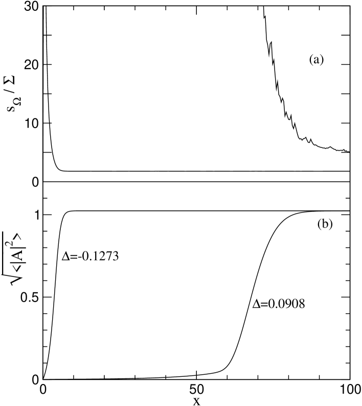
Figure 7: Spatial variation of the standard deviation $s_{\Omega}$ of the frequency reduced by $\Sigma$ (a) and of $\sqrt{<|A|^{2}>}$ (b) for the quintic GLE in the absolutely and convectively regime at $\Delta=-0.1273$ and $\Delta=0.0908$, respectively. After the integration time of $T=5\cdot 10^{5}$ used in this plot $s_{\Omega}$ was for $\Delta=0.0908$ not yet fully stationary in the growth region of $\sqrt{<|A|^{2}>}$. Parameters are $\mu=0.05$ and $\sigma=10^{-3}$.

The downstream reduction of the variance $s_{\Omega}$ of the frequency fluctuations with increasing distance from the inlet and with increasing amplitude along the front is shown in Fig. 7 for the quintic GLE. There we compare the behavior of $s_{\Omega}$ together with the front profiles of $\sqrt{\langle|A|^{2}\rangle}$ in the absolutely and in the convectively unstable regime close to the threshold $\Delta\,=\,0$ for $\mu=0.05$.

IV Conclusion

We have studied numerically the influence of small additive noise on pattern formation near a forwards and near an inverted bifurcation as described by a cubic and quintic GLE, respectively, when a finite group velocity $v$ can blow the finite-amplitude part out of the system, i.e., in the vicinity of the so-called convective-absolute instability at $\Delta=v/v_{c-a}(\mu)-1=0$. The front that connects the inlet condition $A(x=0)=0$ to the finite-amplitude downstream bulk part $\langle|A|^{2}\rangle\simeq R_{N}^{2}$ is for the cubic GLE more sensitive to the applied noise strength than for the quintic case. This is partly related to the different magnitudes of the curvatures of the deterministic GLE potentials around the states $A=0$ and $A=R_{N}$: the resulting growth enhancement of fluctuations near $A=0$ is larger in the cubic than in the quintic case and in addition the damping of fluctuations near $A=R_{N}$ is smaller in the cubic than in the quintic case.

In the cubic case the transition between the regimes of small and large fluctuations of amplitude, frequency, and wave number is shifted to a negative $\Delta$ into the absolutely unstable regime. Simultaneously the pattern growth length $\ell(\Delta)$ has there a characteristic inflection point that shows up as a peak in $\partial\ell/\partial\Delta$. In the quintic case all this occurs at the unshifted convective-absolute threshold $\Delta=0$. Common to both cases is that the fluctuations decrease along the front in both regimes with growing pattern amplitude $\sqrt{<|A|^{2}>}$.

For negative subcritical amplitude growth rates, $\mu<0$, we did not find noise-sustained, large-amplitude, backwards bifurcating patterns when $\Delta$ is positive: the nonlinear deterministic front dynamics of the quintic GLE blows any large-amplitude part downstream away from the inlet where $A=0$ and eventually any finite system is filled only with small-amplitude fluctuations of $A$ around the stable fixed point $A=0$ of the unforced system.

Appendix A

Here we estimate the noise dependence of the downstream growth length $\ell$ of the nonlinear structure in the convectively unstable regime of the cubic GLE where this structure is noise sustained. To that end we approximate $\ell$ by the length where the mean squared amplitude $C_{lin}(x)=\langle|A_{lin}(x)|^{2}\rangle$ of the linear GLE has grown from the inlet value $A(x=0)=0$ to, say, one half of the nonlinearly saturated bulk value $\langle|A|^{2}\rangle\simeq\mu/2$. So we solve the equation

$$C_{lin}(x=\ell)\;=\;\frac{1}{2}\mu\$$ (30)

for $\ell$. Actually the linear solution may not hold there anymore. But as it will become obvious below the result is roughly independent of the coefficient chosen in Eq. (30) so also smaller numbers than $\frac{1}{2}$ could be chosen here for a characteristic growth length.

We evaluate the equal-time correlation $C_{lin}(x)$ via the frequency integral of the spectrum $C_{lin}(x,\omega)$ of the time-displaced autocorrelation function of fluctuations of $A_{lin}$ at the same downstream position $x$. For large downstream distances $x$ from the inlet this spectrum is given by LS97

$$C_{lin}(x,\omega)\;=\;\frac{-\sigma^{2}}{2|K_{1}^{*}-K_{2}|^{2}}\left(\frac{1}{\Im K_{1}}+\frac{1}{\Im K_{2}}\right)e^{-2\Im K_{1}x}$$ (31)

with

$$K_{\binom{1}{2}}\;=\;\pm i\sqrt{\mu_{c-a}-\mu-i\omega}-i\sqrt{\mu_{c-a}}\;.$$ (32)

This spectrum (31) is strongly peaked at the center, $\omega=0$, of the band of modes, $-2\sqrt{\mu\mu_{c-a}}<\omega<2\sqrt{\mu\mu_{c-a}}$, that are amplified in the convectively unstable regime. Thus, the aforementioned frequency integral may be approximated by

$$C_{lin}(x)=\int_{-\infty}^{\infty}\frac{d\omega}{2\pi}C_{lin}(x,\omega)\sim\sqrt{\mu\mu_{c-a}}C_{lin}(x,\omega=0)=\frac{\sigma^{2}}{4\sqrt{\mu}}\exp^{2iK_{1}\left(\omega=0\right)x}\;.$$ (33)

The last equality follows from Eq. (31) at $\omega=0$. Applying now the condition (30) one obtains

$$\ell\;\sim\;\frac{1}{iK_{1}(\omega=0)}\ln{\frac{2^{1/2}\mu^{3/4}}{\sigma}}\;.$$ (34)

Using $\mu_{c-a}/\mu=(1+\Delta)^{2}$ in Eq. (32) one sees that $iK_{1}(\omega=0)=\sqrt{\mu}\left[1-\sqrt{2\Delta}+{\cal O}(\Delta)\right]$ for $\Delta\ll 1$ so that finally at fixed $\mu$

$$\ell\;\sim\;-\left[1+\sqrt{2\Delta}+{\cal O}(\Delta)\right]\left(\ln{\sigma}+const\right)\;.$$ (35)

References

- (1)
- (2) M. C. Cross and P. C. Hohenberg, Rev. Mod. Phys. 65, 851 (1993).
- (3) R. J. Deissler, J. Stat. Phys. 40, 371 (1985).
- (4) K. L. Babcock, G. Ahlers, and D. S. Cannell, Phys. Rev. Lett. 67, 3388 (1991); Phys. Rev. E 50, 3670 (1994); K. L. Babcock, D. S. Cannell, and G. Ahlers, Physica D 61, 40 (1992).
- (5) A. Tsameret and V. Steinberg, Europhys. Lett. 14, 331 (1991); Phys. Rev. Lett. 67, 3392 (1991); Phys. Rev. E 49, 1291 (1994); A. Tsameret, G. Goldner, and V. Steinberg, Phys. Rev. E 49, 1309 (1994).
- (6) H. W. Müller, M. Lücke, and M. Kamps, Phys. Rev. A 45, 3714 (1992).
- (7) W. Schöpf and I. Rehberg, Europhys. Lett. 17, 321 (1992); J. Fluid Mech. 271, 235 (1994).
- (8) M. Lücke and A. Recktenwald, Europhys. Lett. 22, 559 (1993).
- (9) J. B. Swift, K. L. Babcock, and P. C. Hohenberg, Physica A 204, 625 (1994).
- (10) R. J. Deissler, Phys. Rev. E 49, R31 (1994).
- (11) M.Neufeld, D. Walgraef, and M. San Miguel, Phys. Rev. E 54, 6344 (1996).
- (12) M. Lücke and A. Szprynger, Phys. Rev. E 55, 5509 (1997).
- (13) S. P. Trainoff, PhD thesis, UCSB, 1997.
- (14) M. Santagiustina, P. Colet, M. San Miguel, and D. Walgraef, Phys. Rev. Lett. 79, 3633 (1997).
- (15) P. Colet, D. Walgraef, and M. San Miguel, Eur. Phys. J. B 11, 517 (1999).
- (16) A. Bers, in Basic Plasma Physics I, edited by A. A. Galeev and R. N. Sudan (North-Holland, New York, 1983); R. J. Briggs, Electron Stream Interaction with Plasmas (MIT Press, Cambridge, MA, 1964).
- (17) P. Huerre and P. A. Monkewitz, Annu. Rev. Fluid Mech. 22, 473 (1990); J. Fluid Mech. 159, 151 (1985); P. Huerre, in Instabilities and Nonequilibrium Structures, edited by E. Tirapegui and D. Villarroel (Reidel, Dordrecht, 1987), p. 141.
- (18) J. M. Chomaz, Phys. Rev. Lett. 69, 1931 (1992).
- (19) A. Recktenwald, M. Lücke, and H. W. Müller, Phys. Rev. E 48, 4444 (1993).
- (20) H. Brand and R. J. Deissler, Phys. Rev. A 45, 3732 (1992).
- (21) W. van Saarloos and P. C. Hohenberg, Physica D 56, 303 (1992).
- (22) W. H. Press, S. A. Teukolsky, W. T. Vetterling and B. P. Flannery, Numerical Recipes in C, Cambridge: Cambridge University Press (1994).
- (23) S. Kirkpatrick and E. P. Stoll, J. Comput. Phys. 40, 517 (1981); R. C. Tausworth, Math. Comput. 19 201 (1965).