Is it possible to obtain polarized positrons during multiple Compton backscattering process?

A.P. Potylitsyn

Tomsk Polytechnic University
Lenin Ave. 2a, Tomsk, 634050, Russia
E-mail:pap@interact.phtd.tpu.edu.ru

1. In existing projects of electron-positron colliders, the option of polarized electron and positron beams is considered [1,2]. While one can consider the problem of producing the polarized electron beams with required characteristics as having been solved [3], the existing approaches to polarized positrons generation [4-7] do not provide required parameters. In quoted papers the schemes were offered, in which by means of various methods a beam of circularly-polarized (CP) photons with energy of $\sim$ 10¹ MeV is generated to be subsequently used for producing the longitudinally polarized positrons during the process of pair creation in the amorphous converter.

In this paper an alternate approach is discussed - at the first stage the unpolarized positrons are generated by the conventional scheme (interaction of an electron beam with energy of $\sim$10¹ GeV with an amorphous or crystalline converter), which are accelerated up to energy $\sim$ 5 $\div$ 10 GeV and then interact with intense CP laser radiation.

In the scheme of ”laser cooling” of an electron beam suggested in the paper [8], electrons with energy of 5 GeV in head-on collisions with laser photons lose their energy practically without scattering. Thus, as a result of a multiple Compton scattering (MCS), the electron beam ”is decelerated” resulting in some energy distribution, which variance is determined by the electron energy and laser flash parameters. It is clear that the laser cooling process will accompany also the interaction of positrons with laser photons.

If we consider unpolarized positron beam as a sum of two fractions of the identical intensity with opposite signes of 100% longitudinal polarization, its interaction with CP laser radiation results in different Compton effect cross-sections for positrons with opposite helicity. In other words, positrons polarized in opposite directions lose a various part of the initial energy, therefore, by means of momentum selection of the resulting beam, it is possible to get a polarized positron beam with some intensity loss.

2. Let us write the Compton effect cross-section of CP photons on relativistic positrons after summing over scattered photon polarization [9] (the system of units being used hereinafter is $\hbar=m=c=1$):

$$\frac{d\sigma}{dy}=\frac{\pi r^{2}_{0}}{x}\Big{\{}\frac{1}{1-y}+1-y-s^{2}-\xi_{0z}\ P_{c}\ cy\ \frac{2-y}{1-y}\ -$$

$$-\ \xi_{z}P_{c}\Big{[}s_{z}scy+c_{z}\Big{(}\frac{y}{1-y}+yc^{2}\Big{)}\Big{]}+$$ (1)

$$+\xi_{0z}\xi_{z}\Big{[}s_{z}s(1+c^{2}-yc^{2})+c_{z}c\Big{(}\frac{1}{1-y}+(1-y)c^{2}\Big{)}\Big{]}\Big{\}}=$$

$$\frac{d\sigma_{0}}{dy}+P_{c}\ \xi_{0z}\ \frac{d\sigma_{2}}{dy}+P_{c}\ \xi_{z}\frac{d\sigma_{2}}{dy}+\xi_{0z}\ \xi_{z}\frac{d\sigma_{3}}{dy}\;.$$

Here $P_{c}$ is the degree of circular polarization of laser photons, $\xi_{0z}(\xi_{z})$ is the spin projection of an initial (final) positron on the axis $z$ coincident with the direction of the initial positron momentum, $r_{0}$ is the classical electron radius. In (1) standard symbols are used [9]:

$$x=2pk\approx 4\gamma_{0}\omega_{0}\;,\ y=1-\frac{pk^{{}^{\prime}}}{pk}\approx\frac{\omega}{\gamma_{0}}\;,$$

$\gamma_{0}$ is Lorentz factor of an initial positron; $\omega_{0}(\omega)$ is energy of an initial (scattered) photon. The factors $s,c$ are determined in the known way [10]:

$$s=2\sqrt{r(1-r)}\;,\ c=1-2r,\ r=\displaystyle{\frac{y}{x(1-y)}}\;,$$

where as factors $s_{z},c_{z}$ are obtained in going from the coordinate frame related to the momentum of positron scattered through the angle $\theta_{e}$ and used in [9] to the initial one:

$$s_{z}=s-c\ \theta_{e}\;,\ \ \ c_{z}=c+s\ \theta_{e}\;.$$

For an ultrarelativistic case $\theta_{e}=\frac{1}{\gamma_{0}}\ \frac{\sqrt{y(x-y-xy)}}{1-y}$, so with an accuracy of $\sim\gamma_{0}^{-1},\\ s_{z}=s,\ c_{z}=c$.

With the same accuracy, the cross-sections of spin-flip transitions $d\sigma_{+-},\ d\sigma_{-+}$ from states with opposite polarization signs ($\xi_{0z}=+1\to\xi_{z}=-1$ and $\xi_{0z}=-1\to\xi_{z}=+1$) are equal. It means that the Compton scattering process does not result in considerable polarization of an unpolarized beam. It should be remarked that the formula (1) is not the exact invariant expression (as well as formula (12) in paper [9]). Both expressions may be written in the invariant form with an accuracy of $\sim\gamma_{0}^{-1}$. The author’s conclusion [11] concerning the possibility of polarization of a positron beam as a whole through MCS process was incorrect (it was based on the assumption that the magnitude $\int dy\Big{[}\frac{d\sigma_{+-}}{dy}-\frac{d\sigma_{-+}}{dy}\Big{]}$ presents an exact invariant which was calculated in the rest frame of an initial positron, see also [12]).

3. As follows from (1), the total cross-section of positron interaction with CP photons depends on spin projection ($\xi_{0z}$):

$$\sigma=\frac{8}{3}\pi r_{0}^{2}\ [(1-x)-P_{c}\ \xi_{0z}\ \frac{x}{4}]\;.$$ (2)

In many cases of interest (laser cooling, for example) the relation $x\ll$ 1 is satisfied, therefore in (2) the terms $\sim x^{2}$ and higher are discarded. Let’s write the cross-section (2) for 100 % right circular polarization of laser radiation ( $P_{c}$=+1) and for positrons polarized along the photon momentum and in the opposite direction:

$$\sigma_{\pm}=\int\limits_{0}^{x/1+x}\frac{d\sigma_{\pm}}{dy}\ dy\approx\frac{2\pi r^{2}_{0}}{x}\int\limits_{0}^{x/1+x}\Big{[}2-4\frac{y}{x}(1+y)+4\frac{y^{2}}{x^{2}}\big{(}1+2y\big{)}\pm\big{(}2y-4\frac{y^{2}}{x}\big{)}\Big{]}dy\;,$$

$$\sigma_{+}=\sigma(P_{c}=+1,\ \xi_{0z}=+1)=\frac{8}{3}\pi r^{2}_{0}(1-\frac{5}{4}x)=\sigma_{T}\big{(}1-\frac{5}{4}x\big{)},$$ (3)

$$\sigma_{-}=\sigma(P_{c}=+1,\ \xi_{0z}=-1)=\sigma_{T}\big{(}1-\frac{3}{4}x\big{)}\;.$$

Here $\sigma_{T}=\frac{8}{3}\pi r^{2}_{0}$ is the classical Thomson cross-section. It is clear that due to inequality of cross-sections (3), the positrons with various helicities undergo the various number of collisions, that eventually results in difference of average energies $\bar{\gamma}_{\pm}$ of both fractions of the initial unpolarized beam. With this distinction being sufficiently great, and the variance of energy distribution for each fraction being enough small, the polarized positron beam can be generated by means of momentum selection.

4. In paper [13], in considering the MCS process by analogy with passage of charged particles through a condensed medium, the partial equations are derived that describe evolution of average energy $\bar{\gamma}$ and energy straggling (distributions variance) $\Delta$ for unpolarized electron beam passing through an intense laser flash. The approximate analytical solution was derived there as well:

$$\bar{\gamma}=\frac{\gamma_{0}}{1+\displaystyle\frac{\sum^{(1)}l}{\gamma_{0}}}\;,$$

$$\Delta=\frac{\sum^{(2)}l}{\Big{(}1+\displaystyle\frac{\sum^{(1)}l}{\gamma_{0}}\Big{)}^{4}}\;.$$ (4)

In (4) $l$ is the laser flash length (”the thickness” of light target), $\sum^{(n)}$ is the n-order moment of ”macroscopic” interaction cross-section:

$$\sum\nolimits^{(n)}=2n_{L}\ \int\limits_{0}^{\omega_{max}}\omega^{n}\frac{d\sigma}{d\omega}\ d\omega=2n_{L}\gamma_{0}^{n}\int\limits_{0}^{x/1+x}y^{n}\frac{d\sigma}{dy}\ dy\;.$$ (5)

Here $n_{L}$ is the concentration of laser photons, that for ”short” laser flash [8] is estimated as follows:

$$n_{L}=\frac{A}{\omega_{0}}\ \frac{1}{\pi r^{2}_{ph}l}\;,$$ (6)

$A$ is the laser flash energy; $r_{ph}$ is the minimum radius of the laser beam.

Developing (1) as a series in powers of $x$ and retaining two first summands, we get:

$$\sum\nolimits^{(1)}=n_{L}\sigma_{T}\gamma_{0}x\Big{(}1-\frac{21}{10}x\Big{)}\;,$$

$$\sum\nolimits^{(2)}=\frac{7}{10}n_{L}\sigma_{T}\gamma_{0}^{2}x^{2}\Big{(}1-\frac{22}{7}x\Big{)}\;.$$ (7)

After substitution of the found values for $\sum^{(n)}$ in (4) we have:

$$\bar{\gamma}=\frac{\gamma_{0}}{1+n_{L}\sigma_{T}lx\Big{(}1-{\frac{21}{10}}x\Big{)}}\;,$$ (8)

$$\Delta=\gamma_{0}^{2}\ \frac{{\frac{7}{10}}n_{L}\ \sigma_{T}\ l\ x^{2}\Big{(}1-{\frac{22}{7}}x\Big{)}}{\Big{[}1+n_{L}\sigma_{T}lx\Big{(}1-{\frac{21}{10}x}\Big{)}\Big{]}^{4}}\;.$$ (9)

Let’s write the equation (9) in more evident form:

$$\frac{\gamma_{0}}{\bar{\gamma}}=1+n_{L}\sigma_{T}lx\Big{(}1-{\frac{21}{10}x}\Big{)}=1+\frac{1}{2}k_{0}\ x\Big{(}1-{\frac{21}{10}x}\Big{)}\;.$$ (10)

In approximation $x\ll$ 1 the quantity $k_{0}=2n_{L}\ \sigma_{T}\ l$ corresponds to the mean number of scattered photons per an electron of the initial beam (in other words, the average number of collisions of an electron in passing through the ”light” target). When expressing the photon concentration $n_{L}$ in Gaussian laser beam in terms of Rayleigh length $z_{R}$ and the photon wavelength $\lambda_{0}$, defining minimum radius of the ”light” target

$$r_{ph}^{2}=\frac{\lambda_{0}\ Z_{R}}{2\pi}\;,$$

one can readily see that the number of collisions is independent of the laser wavelength directly:

$$k_{0}=\frac{16}{3}\ \alpha\ \frac{A}{mc^{2}}\frac{r_{0}}{Z_{R}}\;,$$

here $\alpha$ is the fine structure constant.

The condition of the approximation applicability (4) (and, therefore, (8) and (9) as well) is written as follows:

$$k_{0}x^{2}\ll 1\;.$$ (11)

The second addend in brackets in (10) can be considered as a correction related to the recoil effect of an initial electron. This correction being neglected, from (10) one can derive the classical result [14]:

$$\frac{\gamma_{0}}{\gamma_{f}}=1+\frac{l}{L_{R}}\;,$$ (12)

$$L_{R}=\Big{(}\frac{8}{3}\ r_{0}\ \gamma_{0}\frac{4\pi^{2}}{\lambda_{0}^{2}}\ a_{0}^{2}\Big{)}^{-1}\;.$$ (13)

In the relationship (12), $\gamma_{f}$ is the electron energy after passing a laser flash; the parameter $a_{0}^{2}$ is determined by the formula (2) in the paper [14]:

$$a_{0}^{2}=3,66\cdot 10^{-19}\ \lambda_{0}^{2}(\mu)\ I(W/cm^{2})\;.$$ (14)

Rewriting (14) in terms of previously derived quantities, we have (for simplicity, here and in the formula (15) dimensional quantities are used)

$$a_{0}^{2}=\frac{1}{\pi}\ \frac{r_{0}}{mc^{3}}\ I\lambda_{0}^{2}=\frac{1}{\pi}\ \frac{r_{0}}{mc^{3}}\ n_{L}\ \omega_{0}\ c\ \lambda_{0}^{2}=2\alpha\ \bar{\lambda}_{e}^{2}\ \lambda_{0}\ n_{L}\;,$$ (15)

$\bar{\lambda}_{e}$ is the Compton wavelength of an electron.

After substitution (14) in (12), the classical expression for characteristic ”thickness” of the light target will be written in terms of quantum characteristics of the laser flash

$$\frac{1}{L_{R}}=\frac{32}{3}\ \pi r_{0}^{2}\ \frac{\gamma_{0}\omega_{0}}{mc^{2}}n_{L}=\sigma_{T}n_{L}x\;.$$ (16)

Thus, the relationship (10) in classical approximation coincides the formula (12), if one compares the average electron energy $\overline{\gamma}$ after the quantum process MCS with the final energy of a particle continuously losing its energy by radiation in travelling along a spiral trajectory in the field of plane electromagnetic wave [15]. For electrons with initial energy $E_{0}$ = 5 GeV having passed through a laser flash of following parameters (see[8]): $\omega_{0}$ = 2,5 eV; $A$ = 5J; $r^{2}_{ph}$ = 4 $\mu m^{2}$, from (10) one can get ${\gamma_{0}}/{\bar{\gamma}}\approx$ 8.7.

Noteworthy is the reasonable agreement with estimates obtained by V. Telnov [8], though the criterion (11) is not satisfied in this case.

Remaining terms proportional $x^{2}$ only the Eq.(9) may be written as

$$\Delta/{\bar{\gamma}}^{2}\simeq 7/10\cdot x{\bar{\gamma}}/\gamma_{0}(1-{\bar{\gamma}/\gamma_{0}})$$

which is rather close to Telnov’s results [8].

5. As it was mentioned above, in ultrarelativistic case the difference between probabilities of spin-flip transitions may be neglected, therefore, in passing the unpolarized positrons through photon beam, the evolution of each fraction of polarized positrons can be considered independently.

In this case, the average energy of a fraction and variance may be written in the full analogy with (4):

$$\bar{\gamma}_{\pm}=\frac{\gamma_{0}}{1+\displaystyle\frac{\sum_{\pm}^{(1)}l}{\gamma_{0}}}\;,$$ (17)

$$\Delta_{\pm}=\frac{\sum_{\pm}^{(2)}\ l}{\Big{(}1+\displaystyle\frac{\sum_{\pm}^{(1)}\ l}{\gamma_{0}}\Big{)}^{4}}\;.$$ (18)

Here by $\sum_{\pm}^{(n)}$ the appropriate cross-section moments are denoted:

$$\sum\nolimits_{\pm}^{(n)}=2n_{L}\ \gamma_{0}^{n}\int\limits_{0}^{x/1+x}\ y^{n}\ \frac{d\sigma_{\pm}}{dy}\ dy\;.$$

The calculation of moments involved in (16) and (17) in the same approximation as before, gives the following result:

$$\sum\nolimits_{+}^{(1)}=n_{L}\ \sigma_{T}\ \gamma_{0}x\Big{(}1-\frac{8}{5}x\Big{)},\ \ \sum\nolimits_{-}^{(1)}=n_{L}\ \sigma_{T}\ \gamma_{0}x\Big{(}1-\frac{13}{5}x\Big{)}\;;$$

$$\sum\nolimits_{+}^{(2)}=\frac{7}{10}\ n_{L}\ \sigma_{T}\ \gamma_{0}^{2}\ x^{2}\Big{(}1-\frac{35}{14}x\Big{)},\ \ \sum\nolimits_{-}^{(2)}=\frac{7}{10}\ n_{L}\ \sigma_{T}\ \gamma_{0}^{2}\ x_{0}^{2}\Big{(}1-\frac{53}{14}x\Big{)}\;.$$

Thus, the relative width of energy distribution in each fraction is deduced from the relations:

$$\frac{\sqrt{\Delta_{+}}}{\bar{\gamma_{+}}}=\frac{\sqrt{\frac{7}{10}n_{L}\sigma_{T}lx^{2}\Big{(}1-\frac{35}{14}x\Big{)}}}{1+n_{L}\sigma_{T}lx\Big{(}1-\frac{8}{5}\ x\Big{)}}=\frac{\sqrt{\frac{7}{20}\ k_{0}\ x^{2}\Big{(}1-\frac{35}{14}x\Big{)}}}{1+\frac{1}{2}k_{0}\ x\Big{(}1-\frac{8}{5}x\Big{)}}\;,$$ (19)

$$\frac{\sqrt{\Delta_{-}}}{\bar{\gamma_{-}}}=\frac{\sqrt{\frac{7}{10}n_{L}\sigma_{T}lx^{2}\Big{(}1-\frac{53}{14}x\Big{)}}}{1+n_{L}\sigma_{T}lx\Big{(}1-\frac{13}{5}\ x\Big{)}}=\frac{\sqrt{\frac{7}{20}\ k_{0}\ x^{2}\Big{(}1-\frac{53}{14}x\Big{)}}}{1+\frac{1}{2}k_{0}\ x\Big{(}1-\frac{13}{5}x\Big{)}}\;.$$ (20)

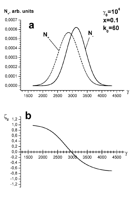
Figure 1: a) Energy distribution of positrons polarized in opposite directions $N_{\pm}(\gamma)$ after passing a laser flash; b) the degree of longitudinal polarization $\xi_{z}(\gamma)$ versus positrons energy.

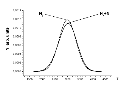
Figure 2: Energy distribution of unpolarized particles $N_{0}(\gamma)$ and the sum of distributions $N_{+}(\gamma)+N_{-}(\gamma)$.

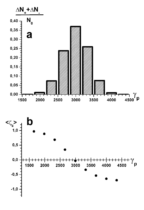
Figure 3: a) Histogram of positron distribution after momentum selection with acceptance $\sigma=\sqrt{\Delta}$ (see Figure 2);  b) the degree of positron longitudinal polarization after momentum selection.

Figure 1a presents the distribution for each fraction after passing the laser radiation with flash parameters: $A$ = 5J;  $\lambda_{0}$ = 1 $\mu$m,   $r_{ph}$= 4.2 $\mu m$($k_{0}$ = 60). The distributions were approximated by Gaussians with parameters (17), (18):

$$\bar{\gamma}_{+}=2868,\ {\sqrt{\Delta_{+}}}/{\bar{\gamma}_{+}}=0.12\;;$$

$$\bar{\gamma}_{-}=3129,\ {\sqrt{\Delta_{-}}}/{\bar{\gamma}_{-}}=0.10\;.$$

The degree of positron polarization being determined in the ordinary way

$$\xi_{z}(\gamma)=\frac{N_{+}-N_{-}}{N_{+}+N_{-}}$$ (21)

is shown in Figure 1b. Figure 2 presents the sum of distributions of both fractions, which practically coincides the distribution for the unpolarized beam with parameters (8), (9). It is evident that only a small portion of positrons in the right (or left) ”tails” of the sum of distributions will have almost 100% longitudinal polarization. By means of momentum analysis with the fixed acceptance $\Delta p/p=\Delta\gamma/\gamma$= const in proximity to a preset value $\gamma_{p}$ one can get a partially polarized positron beam.

Figure 3 presents the polarization degree and intensity of the positron beam resulting from the similar procedure, when after passing a laser flash the beam had characteristics depicted in Figure 1. For simplicity, the calculations were carried out for uniform ”capture”:

$$P=\left\{\begin{array}[]{lll}\rm const,&\gamma_{p}-\displaystyle\frac{1}{2}\sqrt{\Delta}\leq\gamma\leq\gamma_{p}+\frac{1}{2}\sqrt{\Delta}\\ &&\\ 0&\mbox{ off}.\end{array}\right.$$

As follows from Figure 3, positrons with energy in the interval $\gamma$ = 2660 $\pm$ 170 have average polarization $<\xi_{z}>\ \approx$ - 0.35, then in the interval $\gamma$ = 3330 $\pm$170,  $<\xi_{z}>~{}\approx$ 0.34, with the positron intensity in each ”pocket” reaching $\sim$ 24% of the initial one.

It should be noted that in separating the final beam into two parts $(\gamma\leq\bar{\gamma}$ and $\gamma\geq\bar{\gamma})$, the intensity of both beams will be approximately identical (0,5 $N_{0}$ ), and the average polarization decreases only slightly ( $<\xi_{z}>\ \approx\pm$ 0.35).

6. As follows from Figure 2, the noticeable polarization can be reached when the relation below is satisfied:

$$\bar{\gamma}_{+}-\bar{\gamma}_{-}\sim\sqrt{\Delta_{+}}+\sqrt{\Delta_{-}}\approx 2\sqrt{\Delta}\;.$$ (22)

The last relation can be written in a simpler form for rather ”thick” laser target (i.e. under condition $k_{0}\gg$ 1). If in addition to that, the inequality $x\ll$1 is satisfied, in this case

$$\bar{\gamma}_{+}-\gamma_{-}\approx\frac{2\gamma_{0}}{k_{0}}\;.$$

$$\frac{\sqrt{\Delta_{+}}}{\bar{\gamma_{+}}}\approx\frac{\sqrt{\Delta_{-}}}{\bar{\gamma}_{-}}\approx\frac{\sqrt{\Delta}}{\bar{\gamma}}\approx\sqrt{\frac{7}{10}\ x\frac{1}{\frac{1}{2}\ k_{0}\ x}}\sim\frac{1}{\sqrt{k_{0}}}\;,$$

and the criterion (22) can be written in the form:

$$\sqrt{k_{0}}\ x\ \sim 1\;.$$ (23)

In summary it should be noted that the results above were obtained for the linear MCS process. For an essentially nonlinear CS process, when in each act of interaction a positron ”absorbs” $m>$ 1 laser photons, the formulas (18)-(20) will remain valid only in case of satisfying the inequality.

$$\bar{m}x\ll 1\;.$$

Here $\bar{m}$ is the average of absorbed photons in one act of interaction. Evidently that in this case moments $\sum_{\pm}^{(n)}$ should be calculated in terms of nonlinear Compton effect cross-section (see, for example, [16]). Comparing spectra of scattered photons in linear and nonlinear processes [17], one should expect that energy distribution variance of positrons will be higher in the latter case, which can result in increase of ”overlapping” the positron beam fractions $N_{+}$ and $N_{-}$ in comparison with the linear case and, accordingly, in decrease of positron polarization after the selection.

References

• [1] J.E. Clendenin. SLAC-PUB-8465, 2000.
• [2] R.W. Assmann, F. Zimmermann. CERN SL-2001-064.
• [3] J.E. Clendenin, R. Alley, J. Frish, T. Kotseroglou, G. Mulhollan, D. Schultz,
H. Tang, J. Turner and A.D. Yerremian, the SLAC Polarized Electron Source. AIP Conf. Proceedings, No. 421, p. 250 (1997).
• [4] V.E. Balakin, A.A. Mikhailichenko, Preprint INP 79-85, Novosibirsk, 1979.
• [5] T. Okugi, Y. Kurihara, M. Chiba, I. Endo, R. Hamatsu, T.F. Hirose, T. Kumita,
T. Omori, Y. Takeuchi, M. Yoshioka, Jap.J.Appl.Phys. 35, 3677 (1996).
• [6] E.G. Bessonov, A.A. Mikhailichenko, in: Proc. of V European Particle Accelerator Conference, 1996, pp. 1516-1518.
• [7] A.P. Potylitsyn. Nucl. Instrum. and Meth. A398 , 395 (1997).
• [8] V. Telnov. Phys. Rev. Lett. 78 , 4757 (1997).
• [9] G.L. Kotkin, S.I. Polityko, V.G. Serbo. Nucl. Inst. Methods A405, 30 (1998).
• [10] A. Grozin, in: Proc. Joint Int. Workshop on High Energy Physics and Quantum Field Theory. Moscow, 1994, p.60.
• [11] A.P. Potylitsin. Laser polarization of positron beam. Report presented at the ICFA Beam Dynamics Workshop on Laser-Beam Interaction (June 11–15, 2001 at Stony Brook, USA); http://nslserver.physics.sunysb.edu/icfa/Home.htn and LANL arXiv: physics/0203059.
• [12] G.L. Kotkin, V.G. Serbo, V.I. Telnov. LANL arXiV: hep-ph/0205139.
• [13] A. Kolchushkin, A. Potylitsyn, S. Strokov, V. Ababiy. Nucl. Inst. and Meth. B201, 307 (2003).
• [14] E. Esarey. Nucl. Instrum. and Meth. A455, 7 (2000).
• [15] E.S. Sarachik, G.T. Schappert. Phys. Rev. D1, 2738 (1970).
• [16] K.Yokoya. CAIN2e, Code simulation for JHC, Users manual.
• [17] M. Galynskii, M. Levchuk et al. Nucl. Instrum. and Meth. A472, 267 (2001).