Dynamic Point-Formation in Dielectric Fluids

Abstract

We use boundary-integral methods to compute the time-dependent deformation of a drop of dielectric fluid immersed in another dielectric fluid in a uniform electric field $E$. Steady state theory predicts, when the permittivity ratio, $\beta$, is large enough, a conical interface can exist at two cone angles, with $\theta_{<}(\beta)$ stable and $\theta_{>}(\beta)$ unstable. Our numerical evidence instead shows a dynamical process which produces a cone-formation and a transient finite-time singularity, when $E$ and $\beta$ are above their critical values. Based on a scaling analysis of the electric stress and the fluid motion, we are able to apply approximate boundary conditions to compute the evolution of the tip region. We find in our non-equilibrium case where the electric stress is substantially larger than the surface tension, the ratio of the electric stress to the surface tension in the newly-grown cone region can converge to a $\beta$ dependent value, $\alpha_{c}(\beta)>1$, while the cone angle converges to $\theta_{<}(\beta)$. This new dynamical solution is self-similar.

The formation of conical ends on fluid-fluid interfaces in strong electric/magnetic fields has been seen in various electrospraying and ferrofluid experiments zeleny1917 ; taylor1964 ; garton1964 ; fernandez1992 ; nagel2000 ; bacri1982b . Building on the work of Taylor taylor1964 , Li et al. and Ramos & Castellanos studied the electrostatics of an infinite cone with semi-vertical angle $\theta_{0}$ formed between two dielectric fluids with permittivity ratio $\beta$. In spherical coordinates, the electric stress $\sigma_{e}\sim r^{2(\nu-1)}$. In an equilibrium cone, this stress must be balanced by the surface tension, so that $\nu$ must be $1/2$. According to their analysis li1994 ; ramos1994 , there are two such solutions of $\theta_{0}$, $\theta_{<}(\beta)$ and $\theta_{>}(\beta)$, which will occur for $\beta>\beta_{c}=17.59$. The former is said to be stable, the latter unstable li1994 .

In contrast, this letter describes a dynamical fixed point in which a cone is formed transiently. At the fixed point, the cone angle is $\theta_{<}(\beta)$ so that surface stress and electric stress have the same scaling in the cone, with the ratio of the two being constant, but different from unity. The electric stress is the larger of the two, so that the total surface stress always acts to elongate the pointed region.

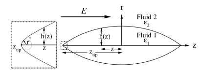
Figure 1: A drop of dielectric fluid freely suspended in another dielectric fluid in a uniform electric field.

We compute the time-dependent deformation of a dielectric drop (fluid 1) freely suspended in another dielectric fluid (fluid 2) in a uniform electric field. Both fluids are incompressible and have the same viscosity $\eta$. There is surface tension with coefficient $\gamma$ between the two fluids. The drop is axially symmetric and has round tips, with its shape represented by the radius function $h(z)$ in cylindrical coordinates $(r,\ z)$. $r^{*}$ denotes the radius of curvature at the tip. An electric field with strength $E$ is applied in the z direction (Fig. 1). Suppose the initial radius of the drop is $a$. Respectively we use $a$, $\gamma/\eta$, $\gamma/a$, $(\gamma/a\epsilon_{o}\epsilon_{2})^{\frac{1}{2}}$ and $(\gamma\epsilon_{o}/a\epsilon_{2})^{\frac{1}{2}}$ to scale length, velocity, stress, electric field and surface charge density sherwood1988 .

Following Sherwood sherwood1988 , we study a situation in which Reynolds number is small so that the fluid flows via Stokes equation and the charge distributions are determined by electrostatics. The surface charge density $\rho$ can be expressed in the form of a boundary integral equation

$$\frac{(\beta+1)}{2(\beta-1)}\rho(x) = \int_{L_{y}}g(x,y)\rho(y)h(y)(1+h^{{}^{\prime}}(y)^{2})^{\frac{1}{2}}dy$$ (1)

$$-\frac{Eh^{{}^{\prime}}(x)}{(1+h^{{}^{\prime}}(x)^{2})^{\frac{1}{2}}},$$

where $\rho(x)$ is the surface charge density at $(h(x),\ x)$, $g$ is a Green function; $\beta$ denotes the permittivity ratio $\epsilon_{1}/\epsilon_{2}$; $L_{y}$ is the range of z axis occupied by the drop sherwood1988 . From the surface charge density $\rho$, the normal and tangential component of the electric field can be calculated to obtain the jump in the electric stress across the interface. Sherwood also uses a boundary integral to determine the interface velocity

$$u_{i}(x)=\frac{1}{8\pi}\int_{L_{y}}G_{ij}(x,y)f_{j}(y)h(y)(1+h^{{}^{\prime}}(y)^{2})^{\frac{1}{2}}dy,$$ (2)

where $i$ and $j$ refer to the $z$ or $r$ component, $f_{j}(y)$ is the $j$ component of the total surface stress, and $G$ denotes a Green function rallison1978 . The velocity, u, is then used to update the interface position. In our simulation, we apply a boundary element method with many details similar to that described by Sherwood. We distribute mesh points in proportion to the local curvature, and use a cubic spline to interpolate the interface between mesh points, a quartic polynomial to interpolate the surface charge density. The derived linear algebraic equations are solved by LU decomposition. A fourth-order Runge-Kutta scheme is applied to update the interface position.

There exists a critical electric field $E_{c}(\beta)$ for $\beta>\beta_{c}$. When $E<E_{c}$, the drop can reach equilibrium with round tips. We start our simulation from a sphere and apply a sufficiently small electric field. If the maximum velocity on the interface decreases to a value below $10^{-4}$ following an exponential decay, we consider that the drop will reach equilibrium. After equilibrium is reached by a numerical extrapolation, the field is increased by a small amount. Through increasing the electric field step by step we find the critical electric field.

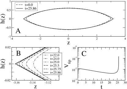
Figure 2: Development of a finite singularity at $\beta=18.5>\beta_{c}$ and $E^{2}=0.410>E^{2}_{c}$. (A) The initial shape (the equilibrium shape at $E^{2}=0.400$), and the final shape calculated ($r^{*}=10^{-12}$). (B) Formation of conical ends. (C) Diverging velocity at the tip.

Figure 3: The shape and stresses at $r^{*}=10^{-8}$ (dashed with dots) and $r^{*}=10^{-10}$ (solid) from the simulation in Fig. 2. (A) Slopes on the interface. (B) Ratios of the electric stress to the surface tension on the interface. $Tan\ \theta_{>}=0.689654$ and $Tan\theta_{<}=0.469704$ at $\beta=18.5$. The later curve matches the earlier one on the right hand parts of the plots.

When $E>E_{c}$, a finite time singularity develops. From now on, we use $\beta=18.5$ as our example, which has $E^{2}_{c}=0.4085\pm 0.0003$. For instance, when we choose the initial shape to be the equilibrium shape at $E^{2}=0.400<E^{2}_{c}$ and suddenly apply $E^{2}=0.410>E^{2}_{c}$, the drop forms conical-like ends. The velocity at the tip dramatically increases as a critical time is approached (Fig. 2). Here we can at most obtain about twelve decades of data in one calculation, due to the increasing number of mesh points required and roundoff error.

Figure 3 shows how the shape and stresses evolve as the finite time singularity develops. The slope plot suggests we can partition the interface into three regions, the tip region, the conical-like region and the macroscopic region. The conical-like region is the intermediate region with a small variation in the slope. Figure 3(A) shows as $r^{*}$ decreases, the macroscopic region and the established part of the cone region almost remain intact, while part of the interface which used to be in the tip region now grows conical-like. This shows that in the course of $r^{*}\to 0$, only the tip region changes in time, while the established part of the cone region nearly remains independent of time. A careful examination of Fig. 3(A) shows the conical-like region is not exactly a cone, because the slope of the newly-grown cone changes as $r^{*}$ decreases. As we shall see in more detail later, this slope approaches the value set by $\theta_{<}$. Figure 3(B) shows the ratio of the electric stress to the surface tension is larger than one in the tip region and the conical-like region. The stress ratio also does not change in the part of interface whose shape remains as the conical-like region expands. Hence the numerical evidence says that the shape of each part of the almost conical region and the stress ratio within that part remain frozen as the tip gets smaller. However, as $r^{*}$ changes the slope and the stress ratio of the newly-grown part change too. So Figure 2 and 3 may show an approach to a fixed point, but they do not show a fixed behavior themselves. Because there is a slow and not-quite uniform convergence to a fixed point, it is hard to estimate the critical time, $t_{c}$, from our raw data. For this reason, we shall henceforth plot our results against tip radius, $r^{*}$ instead of trying to use $t_{c}-t$.

A scaling study, sometimes called an order of magnitude analysis, enables us to estimate the sizes of different contributions, it indicates how the different regions affect one another.

These estimates show that except for a uniform advection, the stresses in the tip region determines the flow within that region and the subsequent shape of the tip. Specifically, the deformation of the tip region is dominantly caused by the local stress jump. The axial strain rate defined as $\partial u_{z}(x)/\partial x$ measures how fast the interface deforms due to the axial velocity. Using (2), we can express the contribution to $\partial u_{z}(x)/\partial x$ from the three regions. Respectively the tip region, the conical region and the macroscopic region have length scales $r^{*}$, $h(z)$ and $1$ ($r^{*}\ll h(z)\ll 1$). The electric stresses in the three regions have an order of magnitude

$$\sigma_{e}\sim\rho^{2}\sim\left\{\begin{array}[]{ll}E^{2}\ r^{*2(\nu-1)}&\mbox{tip region}\\ E^{2}\ h(z)^{2(\nu-1)}&\mbox{conical-like region,}\\ E^{2}&\mbox{macroscopic region}\end{array}\right.$$ (3)

with $0<\nu<1$. A similar result applies to the surface tension $\sigma_{s}$, but with $\nu=1/2$. An argument like that of Lister and Stone shows that the forces in the intermediate and macroscopic region simply advect the tip region without significant contribution to the strain rate lister1998 .

A followup study yang2002 will describe in more detail how the scaling analysis of the electric stress works. For the present purposes, it suffices to say that the shape in the tip region mostly determines the electric stress within that region, except for a coefficient which only depends on the shape in the other regions and the applied electric field. If we change the shape in the other regions, the electric stress in the entire tip region will be changed by a factor which is independent of the shape in the tip region. Changing the applied electric field will have the same effect. So after we reshape the rest part of the interface, we can restore the electric stress in the tip region by applying a different electric field of certain strength.

The scaling study permits us to construct approximate boundary conditions which then permits the accurate determination of the subsequent behavior of the tip. Basically whenever we are about to run out of mesh points, we cut off the part of interface far away from the tip and replace it by a new shape profile which takes fewer mesh points. Then we restore the electric stress in the entire tip region, which we can accomplish by adjusting the applied electric field to restore the electric stress at the tip to its value prior to the truncation. The tip regions of the prescribed new drop and the original drop will subsequently evolve in the same way, because the deformation of the tip region is primarily driven by the local stress jump. We define the rescaled axial distance $\xi$ and radius function $H(\xi)$ as

$$\xi=(z-z_{tip})/r^{*},\qquad H(\xi)=h(z)/r^{*}.$$ (4)

We at least keep the part of interface with $\xi\leq 10^{4}$ and typically match a spherical band to the center region, requiring the slope to be continuous at the truncation points. The center of the spherical band, which locates on the z axis, coincides with the center of the prescribed new drop. The error will be smaller if the truncation point is farther away from the tip. The “truncate and prescribe” idea was invented by Zhang and Lister zhang1999 .

Figure 4: Overlap between the results calculated with the exact boundary condition (solid curves) and the approximate boundary condition (dotted curves). The initial condition is given in Fig. 2. Evolution of the tip region is calculated for totally $80$ decades of $r^{*}$, only part of which are shown here. Out of the $80$ decades of data, the curves at small $r^{*}$ converges as power laws in $r^{*}$. The fit shows as $r^{*}\to 0$: (A) The slope at $\xi=100$ converges to $0.47260\pm 0.00003$, (B) the stress ratio at $\xi=100$ converges to $1.1302\pm 0.0004$, and (C) $dr^{*}/dt$ converges to $-0.01977\pm 0.00003$.

Figure 5: Convergence to a fixed point at $\beta=18.5$. The initial shape and the applied field of simulation (i) in solid lines: a sphere, $E^{2}=0.4748$; simulation (ii) in dotted lines: a sphere, $E^{2}=0.473$; simulation (iii) in dashed lines: the equilibrium shape at $E^{2}=0.408$, currently $E^{2}=0.478$. The overlap between the approximate boundary condition results and the exact boundary condition results is similarly checked like in Fig. 4. As $r^{*}\to 0$, (A) $H^{\prime}(\xi=100)\to 0.472595\pm 0.000005$; (B) $\alpha(\xi=100)\to 1.13040\pm 0.00004$; (C) $dr^{*}/dt\to-0.019780\pm 0.000003$.

Using the same initial condition as in Fig. 2, we calculate the evolution of the tip region for eighty decades of $r^{*}$ with approximate boundary conditions. We truncate the drop for twenty-four times, starting at $r^{*}=10^{-8}$. Figure 4 shows that the approximate boundary condition produces the same result as the exact boundary condition without truncation at $10^{-12}\leq r^{*}\leq 10^{-8}$. The point with $\xi=100$ is pretty close to the cone region, so the slope and the stress ratio there can respectively reflect the angle and the stress ratio of the newly-grown cone. Out of the eighty decades of data, the curves at small $r^{*}$ can be adequately fitted as $c+b(r^{*})^{p}$ with $p>0$. Thus $H^{{}^{\prime}}(\xi=100)$, $\alpha(\xi=100)$ and $dr^{*}/dt$ each approach limiting values as $r^{*}\to 0$. Just below we shall show those limits are the same for different initial conditions.

Further simulations show there exists a fixed point behavior: the stress ratio of the newly-grown cone converges to a fixed value larger than unity. At $\beta=18.5$, $\alpha(\xi=100)$ will converge to $1.130$ as $r^{*}\to 0$, if it is close to $1$ when the drop starts to develop conical ends, regardless of the initial shapes. For example in Fig. 5, simulation (ii) in solid lines and simulation (iii) in dashed lines have different initial conditions. The dotted lines and dashed lines can all be excellently fitted by $c+b(r^{*})^{p}$. As $r^{*}\to 0$, the two simulations give the same limits $H^{{}^{\prime}}(\xi=100)_{c}=0.4726$, $\alpha(\xi=100)_{c}=1.130$ and $(dr^{*}/dt)_{c}=-0.0198$. As you may notice, we have obtained the same limits in the simulation in Fig. 4. The fitted values of the power are very close to each other in all the simulations, and we get $p=0.013\pm 0.001$. In simulation (i), we purposely choose a particular initial condition to let $\alpha(\xi=100)$ equal to $\alpha(\xi=100)_{c}$ at an early stage in the cone formation. We see that $\alpha(\xi=100)$ stably stays at $\alpha(\xi=100)_{c}$ for many decades of $r^{*}$ with $H^{{}^{\prime}}(\xi=100)$ and $dr^{*}/dt$ equal to the limits obtained from the curve fitting. We have concrete numerical evidence that $\alpha(\xi=100)_{c}=1.130$ is a stable fixed point at $\beta=18.5$. This fixed point is finally approached in a power law of $r^{*}$. And simulation (i) gives the solution at this fixed point.

Figure 6: The self-similar solution at the fixed point $\alpha(\xi=100)_{c}=1.130$ at $\beta=18.5$. The first $12$ decades of data computed with the exact boundary condition in simulation (i) reveal: (A) $H(\xi)$ is a constant for small $r^{*}$, for example at $\xi=10$. (B) The intermediate region has a constant slope $0.46970$ nearly equal to $Tan\ \theta_{<}(18.5)=0.469704$. (C) The velocity at the tip increases logarithmically. (D) The stress ratio in the intermediate region is a constant $1.130>1$. In (B)(D), dashed curves: $r^{*}=10^{-8}$, solid curves: $r^{*}=10^{-12}$.

At this fixed point, the tip region is self-similar and the intermediate region is a cone with the cone angle $\theta_{<}(\beta)$. The first twelve decades of data calculated with the exact boundary condition in simulation (i) reveal the solution at this fixed point. We find the following properties: (a) The shape profiles of the tip region are self-similar after we rescale them by $r^{*}$, for example $H(\xi)$ at $\xi=10$ is a constant for small $r^{*}$ [Fig. 6(A)]. (b) The ever expanding intermediate region has a constant slope equal to $Tan\ \theta_{<}(\beta)$ [Fig. 6(B)]. (c) The velocity at the tip increases logarithmically [Fig. 6(C)]. (d) The stress ratio in the intermediate region is a constant substantially larger than one, which we call it $\alpha_{c}$ [Fig. 6(D)]. The values of $\alpha_{c}$ and $\alpha(\xi=100)_{c}$ are very close to each other. (e) $dr^{*}/dt$ is a constant [Fig. 5(C)], which indicates that $r^{*}$ scales like $t_{c}-t$. This self-similar solution has some qualitative similarity with a scaling solution found by Lister and Stone lister1998 .

We find similar fixed points at other values of $\beta>\beta_{c}$ such as $19.0$. To summarize, our numerical evidence shows a cone with the smaller cone angle $\theta_{<}(\beta)$ can be formed transiently in a non-equilibrium case where the electric stress is not balanced by the surface tension. The angle is approached as the stress ratio in the newly-grown cone region converges to a fixed value $\alpha_{c}(\beta)>1$. The dynamical solution at this fixed point is self-similar.

This project would be simply impossible without Leo P. Kadanoff’s guidance and support. I am very grateful to H. A. Stone and W. W. Zhang for their codes on viscous pinchoff. I also want to thank W. W. Zhang for helpful discussions. This research was supported in part by the DOE ASCI-FLASH program, the NSF grant DMR-0094569 to L. P. Kadanoff, and the MRSEC program of the National Science Foundation under Award No. DMR-9808595.

References

- (1) J. Zeleny, Phys. Rev. 10, 1 (1917).
- (2) G.I. Taylor, Proc. R. Soc. Lond. A 280, 383 (1964).
- (3) C.G. Garton and Z. Krasucki, Proc. R. Soc. Lond. A 280, 211 (1964).
- (4) J. Fernández de la Mora, J. Fluid Mech. 243, 561 (1992).
- (5) L. Oddershede and S.R. Nagel, Phys. Rev. Lett. 85, 1234 (2000).
- (6) J.C. Bacri and D. Salin, J. Phys. Lett. 43, 649 (1982).
- (7) H. Li, T. Halsey and A. Lobkovsky, Europhys. Lett. 27, 575 (1994).
- (8) A. Ramos and A. Castellanos, Phys. Lett. A 184, 268 (1994).
- (9) J.D. Sherwood, J. Fluid Mech. 188, 133 (1988).
- (10) J.M. Rallison and A. Acrivos, J. Fluid Mech. 89, 191 (1978).
- (11) J.R. Lister and H.A. Stone, Phys. Fluids 10, 2758 (1998).
- (12) C. Yang and L.P. Kadanoff, in progress (2003).
- (13) W.W. Zhang and J.R. Lister, Phys. Rev. Lett. 83, 1151 (1999).