Neutrino Oscillations for Dummies

Abstract

The reality of neutrino oscillations has not really sunk in yet. The phenomenon presents us with purely quantum mechanical effects over macroscopic time and distance scales (milliseconds and 1000s of km). In order to help with the pedagogical difficulties this poses, I attempt here to present the physics in words and pictures rather than math. No disrespect is implied by the title; I am merely borrowing a term used by a popular series of self-help books.

I Introduction

Within the last two years, neutrino oscillations, first postulated in 1969, have become a reality. The consequences for our view of particle physics, astrophysics, and cosmology, are quite profound. However, even for physicists, an understanding of the evidence for oscillations and their mechanism can be elusive. This article aims to present the current state of our knowledge of neutrino oscillations in as simple a way as possible. It is a result of preparing for my talk at the American Association of Physicists winter meeting of 2003, and of teaching the 4th-year particle physics course at UBC. A lot of verbiage common to the neutrino oscillation industry will be explained. For brevity and simplicity I will only look at what is currently the most likely scenario for neutrino masses and mixings; other possibilities are shamelessly ignored. The hope is that this treatment will be accessible to physics teachers and other non-specialists. The reader is warned however that this text is dense; most sentences contain some essential ingredient. My bibliography aims at accessibility rather than rigour or completeness. I present one mathematical equation.

II Quarks and Leptons

The fundamental constituents of matter as we know it come in pairs - “doublets” - of elementary particles which are very similar to each other except that their charges differ by one fundamental unit. That unit is the magnitude of the charge on the electron, which is the same as that on the proton. The first hint that the universe is structured this way came when it was recognized that atomic nuclei are formed of protons and neutrons, which are more-or-less identical particles except that one has a charge of +1 and the other a charge of zero. We now understand these particles in terms of their elementary constituents, the quarks. The proton has two “up”-quarks ($u$, charge +2/3) and one “down”-quark ($d$, charge -1/3); the neutron has two downs and an up. In addition to these light, stable quarks, there are two more doublets which have larger mass, and are unstable, eventually decaying into ups and downs. These are called charm ($c$, +2/3) and strange ($s$, -1/3), top ($t$, +2/3) and bottom ($b$, -1/3). The names have no meaning, except to keep physicists all talking the same language. So we have three “generations” of quark “flavours”, and this arrangement has deep significance for the structure of the universe. Too deep to go into here.

$(u,d),(c,s),(t,b)$

The link between the partners in the doublets is the weak-interaction, the fundamental force which controls $\beta$-decay, and, as we shall see, solar fusion reactions. The weak-interaction allows a $d$ to turn into a $u$ etc., where energy considerations permit. Significantly, it allows a free neutron ($n$) to ($\beta$-)decay into a proton ($p$) and an electron ($e^{-}$, historically known as a $\beta$-ray).

$$n\rightarrow p+e^{-}+\bar{\nu}_{e}$$ (1)

Or, in terms of the quarks (with the spectators in parentheses):

$$u(ud)\rightarrow d(ud)+e^{-}+\bar{\nu}_{e}$$ (2)

We’ll get to the $\nu_{e}$ in a second. Suffice it to say that without neutron decay there would be no free hydrogen in the universe, and we would probably not be around to worry about neutrinos.

These flavour states ($u,d,c,s,b,t$) - we call them “eigenstates” - are not kept rigidly separate. The states in which these quarks propagate are called “mass eigenstates”, which are each different mixtures of the flavour eigenstates. The mass eigenstates propagate at different speeds and so the components get out of phase with each other. A quark born as one flavour will soon start looking like another. An $s$-quark travelling through space can turn into a $d$-quark. Likewise all the right-hand partners can mix between the generations, and any particle made of 2nd or 3rd-generation quarks can decay into a stable particle made of 1st-generation quarks. By convention we push all the mixing into the right-hand partner; this is allowed because the weak-interaction allows transformations between the left and right partners anyway.

So much for the structure of heavy particles (baryons), those which form much of our mass. What about the light particles (leptons), starting with the electron? There are three charged leptons - electron, muon and tau - and three associated very light chargeless neutrinos, clearly separated by one unit of charge.

$(e^{-},\nu_{e}),(\mu^{-},\nu_{\mu}),(\tau^{-},\nu_{\tau})$.

Superficially this organization looks very much like the quarks. However, for a long time the neutrinos were thought to be massless (as no mass had been detected). In this case, no mixing is possible, as all neutrinos will propagate at precisely the speed of light, and the mass eigenstates can never get out of phase with each other. An electron neutrino born will never change its composition, as all parts will move at the same speed, and so the neutrino can never be detected as any other flavour.

As it turns out, this is not the case.

Mixing of flavours in the charged leptons would be easy to see. Muons would decay into electrons and gamma-rays; this would be a fast electromagnetic decay in contrast to the slow weak decay which actually happens.

$$\mu^{\pm}\rightarrow e^{\pm}+\gamma$$ (3)

$$\mu^{+}\rightarrow e^{+}+\bar{\nu}_{\mu}+\nu_{e}\ \ \mbox{or}\ \ \mu^{-}\rightarrow e^{-}+\nu_{\mu}+\bar{\nu}_{e}$$ (4)

The first decay violates lepton flavour and has never been seen. The second decay tortuously conserves lepton number, and is the way all muons seem to decay.

III Early Indications (1968-1992)

By the 1960s our understanding of the solar interior, and of low energy nuclear physics, had reached such a stage that the Sun’s neutrino output could be predicted with some confidence. In broad terms, this picture remains unchanged to this day. For an excellent review of the subject in somewhat more mathematical detail the reader is directed to an article by K. Nakamura in the Particle Data Booknakamura , which is available online.

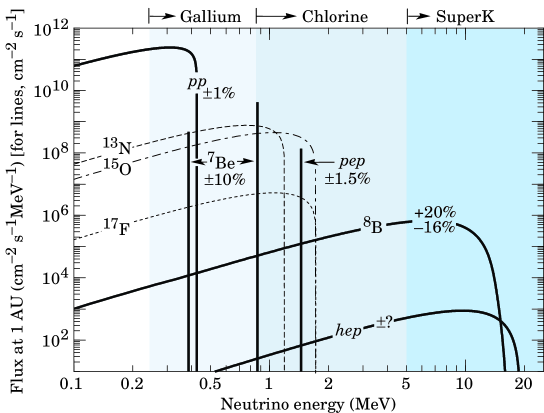
Figure 1: The solar neutrino spectrum, showing the contribution of the ⁸B and pp processes, and the thresholds for the three detection mechanisms. The figure is reproduced by courtesy of the Particle Data Group. pdg ; bahcall

The two most important reactions - both weak - yield the copious, low energy “pp” neutrinos, and the more scarce high energy “⁸B” neutrinos (see fig.1).

$$p+p\rightarrow\mbox{D}+e^{+}+\nu_{e}\ \ \ \ E_{\nu}=0-0.420\mbox{ MeV}$$ (5)

$${}^{8}\mbox{B}\rightarrow 2^{4}\mbox{He}+e^{+}+\nu_{e}\ \ \ \ E_{\nu}=0-14.6\mbox{ MeV}$$ (6)

The “D” is a deuteron, heavy hydrogen ²H. The pp-neutrinos are very hard to see, even by neutrino standards, and can only be detected by radio-chemical means (see below). However their flux (about 10¹⁵ m^-2s^-1 at the Earth) is 10,000 times that of the ⁸B-neutrinos. (An MeV is a million electron volts, a typical energy release for a single nuclear reaction.)

Now the experimental nuclear physicists took up the challenge to detect these elusive particles.

III.1 Neutrino Detection

The chargeless neutrino cannot be “seen” unless it is (a) absorbed on a nucleon and produces a charged lepton, or (b) scatters on an electron. In both cases the reaction products may be seen - always through their electromagnetic properties. There are two fundamental ways of detecting a neutrino; either by scattering off a nucleon, or an electron.

III.1.1 Nucleons

Electron-type neutrinos can scatter off a neutron to produce a proton, and the other half of the neutrino’s doublet, the electron. This is a charge-swapping “quasi-elastic” reaction.

$$\nu_{e}+n\rightarrow e^{-}+p$$ (7)

This reaction is exothermic, as the chemists would have it, and so would be accessible to all solar neutrinos. Unfortunately, free neutrons don’t live much longer than a quarter of an hour, and so a macroscopic detector is hard to build. The reaction doesn’t work on protons (hydrogen would be a convenient detector) because the charges cannot be made to match (it will for anti-neutrinos, which can make positrons - $e^{+}$).

The next best thing is to use neutrons in a nucleus. This is not easy as protons are usually bound less tightly in a nucleus than are neutrons, and so their effective mass increases and this raises the energy threshold for the reaction, in most cases out of reach of solar neutrinos. In addition, the outgoing electron is usually too low in energy to see, and so one has to rely on a detectable product nucleus. This means it has to be physically removable from the detector and radioactive with a convenient-enough half-life (preferably days) to accumulate and to observe after removal. In fact the reaction tends to make a nucleus which is too proton-rich, and these do tend to decay by the slow process of atomic-electron capture, which produces detectable X-rays. The basic decay process is the reverse of neutrino absorption and yields back the original nucleus:

$$e^{-}+p\rightarrow\nu_{e}+n$$ (8)

In addition, the weakness of the weak interaction means we need 100s or 1000s of tonnes of target material to get a good signal, so the substance has to be cheap, safe and purifiable of trace radioactivity. Three nuclei have been used as detectors to date. The first was chlorine-37, in the form of borrowed cleaning fluid, which has been used by Ray Davisdavis since the late ’60s:

$$\nu_{e}+^{37}\mbox{Cl}\rightarrow e^{-}+^{37}\mbox{Ar}$$ (9)

This method of detection is sensitive to most of the ⁸B spectrum and neutrinos from some intermediate reactions. The radioactive argon, a noble gas, can be bubbled out of the chlorine using helium. It decays by the capture of an atomic electron, a process which kicks out further atomic (“Auger”) electrons which can be detected and counted.

$$e^{-}+^{37}\mbox{Ar}\rightarrow\nu_{e}+^{37}\mbox{Cl}+\mbox{Auger electrons}$$ (10)

This was the first successful detection method for solar neutrinos, and as a result, Davis shared the 2002 Nobel Prize in Physicsnobel .

The only detector successfully used to date which can see the pp-neutrinos is gallium-71. The first results were recorded by the Soviet-American Gallium Experiment SAGEsage , and the Italo-German Gallex gallex , in 1990.

$$\nu_{e}+^{71}\mbox{Ga}\rightarrow e^{-}+^{71}\mbox{Ge}$$ (11)

It works like the chlorine reaction except that gallium is converted to radioactive germanium eve. However, you can’t bubble germanium out of liquid gallium without first converting it to a gas. This has been done, but it requires more chemistry than you can shake a stick at. Wags call the gallium-germanium-gallium sequence the “Alsace-Lorraine” process, but don’t tell this to an undergraduate class unless you want rows of blank faces.

The third useful nucleus is deuterium, but in a different way. The proton and neutron are bound in deuterium so lightly that the electron is energetic enough to be visible. This is fortunate, because the stable protons are not:

$$\nu_{e}+\mbox{D}\rightarrow p+p+e^{-}$$ (12)

The most convenient form of deuterium is heavy water (not cheap but at least availabled2o ), and the fast electron emits Cherenkov radiation which can be readily detected. Cherenkov radiation is the result of a charged particle travelling at faster than the local speed of light (in water = c/1.33) which emits the electromagnetic equivalent of a supersonic boom, a conical pattern of blue and UV photons. The first such heavy water Cherenkov detector is the Sudbury Neutrino Observatory (SNO)SNO , and it started operating in 1999, a decade after the first light water Cherenkov detector, Kamiokande (see next section).

III.1.2 Electrons

Conceptually the simplest way to detect neutrinos is via elastic scattering off electrons, which are plentiful in any material. One simply has to choose a cheap, safe, purifiable, transparent medium so the Cherenkov light from neutrinos can be distinguished from the inevitable trace radioactivity. Water works well. The masters of this technique are the Japanese Kamiokande collaboration (and its successor, SuperKamiokande). Kamiokande announced the first real-time, directional detection of solar neutrinos in 1989kamII . It was for initiating this series of experiments that Masatoshi Koshiba shared the 2002 Nobel Prize in Physicsnobel . The reaction is:

$$\nu_{e}+e^{-}\rightarrow\nu_{e}+e^{-}$$ (13)

Undergraduates have complained to me that this is not a real reaction because the left hand side is the same as the right (and get even more confused if I occasionally leave the $+$ signs out). They have obviously been made to sit through too many chemistry lectures. The left-hand electron is stationary, while the right-hand one is recoiling from the neutrino and is moving close to the speed of light, which makes it visible. The directionality comes from the fact that the recoil electron tends to travel in line with the original neutrino. This method of detection is sensitive to the upper end of the ⁸B spectrum.

There’s a slight but significant complication here. Electron scattering also works for muon and tau neutrinos, e.g.:

$$\nu_{\mu}+e^{-}\rightarrow\nu_{\mu}+e^{-}$$ (14)

The cross-section (i.e. sensitivity) of this reaction is only 15% of that for electron neutrinos.

III.1.3 The Data

By 1990, the chlorine, light water, and gallium experiments (in that order), had all reported seeing only a small fraction of the expected signal. The numbers are given below. Note that all these experiments have to be done deep underground, to get away from cosmic rays which would easily swamp the tiny neutrino signal on the surface.

• Gallium (0.2 MeV threshold) - 55%

• Chlorine (0.8 MeV threshold) - 34%

• Light Water (9 MeV threshold, later 5 MeV) - 48%

There were 10-20% errors in these numbers due to experimental and theoretical uncertainties, but it was clear that none of these numbers was remotely consistent with 100%. By this time, the solar astrophysicists were getting very confident of their flux predictions, and so these deficits became known as the “Solar Neutrino Problem”. When physicists use the word “problem”, they mean “funding opportunity”.

IV Pontecorvo’s Idea

All the above detection reactions are sensitive only to $\nu_{e}$ (with the one exception noted). In 1969 Bruno Pontecorvo reasoned that if neutrinos had small and different masses, plus flavour mixing, then $\nu_{e}$s born in the Sun might reach Earth as, say $\nu_{\mu}$ ($\nu_{\tau}$s were not known then) and be undetectablebp . This might be the answer to the emerging Solar Neutrino Problem.

For simplicity, consider two neutrino species. Neutrinos are born and detected via the weak interaction as “flavour eigenstates”, e.g. $e$ and $\mu$ . However they propagate as “mass eigenstates” which have a distinct velocity, labelled, for example, “1” and “2”

If flavour is not rigorously conserved (there is no particular reason why it should be, except that’s the way the charged leptons seem to behave), and if the masses $m_{1}$ and $m_{2}$ are slightly different, these two pairs of states may not be one and the same, but may be mixed:

$$\nu_{1}=\nu_{e}\cos\theta+\nu_{\mu}\sin\theta\ \ \ \ \ \nu_{2}=\nu_{e}\sin\theta+\nu_{\mu}\cos\theta$$ (15)

Our use of sines and cosines of an angle ensures that the mixing produces neither more or less neutrinos than we started with. Its called a “unitary” transformation because the particle number depends on the square of the amplitude terms shown ($\cos^{2}+\sin^{2}$ is always 1 - Math 10). We will define the phrase “slightly different” later. Consider a neutrino which was created as an electron neutrino. The probability that it will be detected as an electron neutrino a distance $L$ away is (after a bit of math):

$$P_{ee}=P_{\mu\mu}=1-\sin^{2}2\theta\sin^{2}k\Delta m^{2}L/E$$ (16)

Numerically, the constant $k=1.27$ if $\Delta m^{2}=m_{2}^{2}-m_{1}^{2}$ is measured in eV² (strictly eV/$c^{2}$ all squared, from $E=mc^{2}$ - but we like to think $c$ = 1), the energy $E$ in MeV and the distance from the source $L$ in m. It will equally work for GeV and km. These are classical “vacuum oscillations”, and they are plotted for the parameters we now associate with solar neutrinos in fig.2.

With three species, the mass and flavour basis states are linked via a $3\times 3$ matrix with two mass splittings, three angles like $\theta$ and an extra one which makes life different for neutrinos and antineutrinos (a “CP-violating phase”).

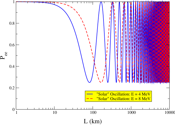
Figure 2: The probability $P_{ee}$ is plotted against the distance between the source and detection for two monoenergetic electron neutrinos, at 4 MeV (typical detected reactor neutrino energy) and at 8 MeV (typical detected solar neutrino energy). Both have the currently accepted solar oscillation parameters of $\Delta m^{2}_{S}=6\times 10^{-5}$ and $\theta=\pi/6$. It is clear that a reactor experiment, with a neutrino spectrum several MeV wide, will see no effect below 10 km, but at further than 100 km will see about 60% of the unoscillated flux.

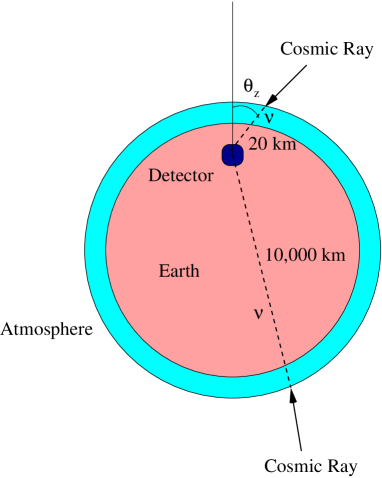
Figure 3: The production mechanism and geometry for the detection of atmospheric neutrinos.

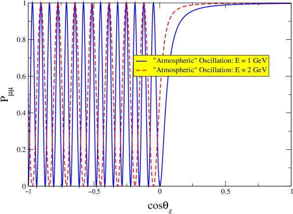
Figure 4: The probability $P_{\mu\mu}$ is plotted against the cosine of the zenith angle $\theta$ for the case of an atmospheric neutrino experiment. Neutrinos coming from directly above have $\cos\theta=+1$, those from the nadir have $\cos\theta=-1$. The energies plotted are 1 and 2 GeV (typical values in this case) with the accepted atmospheric oscillation parameters of $\Delta m^{2}_{A}=3\times 10^{-3}$ and $\theta_{A}=\pi/4$. It is easy to see that with an atmospheric neutrino spectrum a few GeV wide, there will be no effect on $\nu_{\mu}$ flux above the horizontal, but only 1/2 of the expected $\nu_{\mu}$ flux will be seen below the horizontal.

V The Hard Evidence, 1992-2002

There are now two widely recognized pieces of evidence for neutrino oscillations:

• the atmospheric muon-neutrino deficit

• the solar electron-neutrino deficit

The first was formally announced by the Kamiokande collaboration in 1992 kamiokande . It was declared to be proof of non-zero neutrino mass (consistent with oscillations) in 1998 by that collaboration’s successor, SuperKamiokande SK . Evidence for the latter had been building steadily over 30 years, but proof came in 2001/2 by the Sudbury Neutrino Observatory collaborationsno2002 , who showed that solar astrophysics could not be to blame for the deficit, and that the “missing” neutrinos were arriving at the Earth as other flavour states. The particular oscillation mechanism suggested by the solar experiments was confirmed in December 2002 by the KamLAND reactor-neutrino detector, a fact which removed any lingering worries about uncertainties due to solar astrophysics.

We will call the neutrino parameters revealed by atmospheric neutrinos $\Delta m^{2}_{A}$ and $\theta_{A}$, and those revealed by solar (and reactor) neutrinos $\Delta m^{2}_{S}$ and $\theta_{S}$. The remaining angle (“$\theta_{13}"$) is now very much sought after. The CP-violating phase is even hotter property but it will be very hard and expensive to findjhf .

V.1 Atmospheric Neutrinos

Atmospheric neutrinos are made by pion and kaon decays resulting from cosmic-ray interactions in the upper atmosphere. The numerology of these decays leads one to expect two $\nu_{\mu}$s for each $\nu_{e}$ (it is very hard experimentally to distinguish between neutrinos and antineutrinos, ($\bar{\nu}$). The following reaction sequence is typical:

$$p+^{14}\mbox{N}\rightarrow\pi^{+}+X\ \ \ \ \ \pi^{+}\rightarrow\mu^{+}\nu_{\mu}\ \ \ \ \ \mu^{+}\rightarrow e^{+}\nu_{e}\bar{\nu}_{\mu}$$ (17)

Here $X$ means nuclear fragments. However, the observed $\mu/e$ ratio is more like unity on average, and is strongly dependent on zenith angle i.e. the distance the neutrino has travelled since birth (fig.3). It seems that the further a $\nu_{\mu}$ travels in the Earth, the less chance it has of being detected, even though the probability of absorption is tiny. In fact the mean free path of an atmospheric neutrino in rock is about $10^{12}$ m, so only a tiny fraction interact in the Earth with its diameter of only $10^{7}$ m. Therefore they must be disappearing by some other means.

The measured flux of $\nu_{\mu}$s is about half the expected value, while that for the $\nu_{e}$s is about right. There are strong indications from SuperKamiokande (SK) that the missing $\nu_{\mu}$s are showing up as $\nu_{\tau}$s (which are very hard to see). We will assume this is the case.

Detailed analysis in terms of path length through the Earth yields an L/E dependence as expected from the eq.16, with parameters:

$$\Delta m^{2}_{A}\approx 3\times 10^{-3}\mbox{ eV}^{2}\ \ \ \ \ \theta_{A}\approx\pi/4$$ (18)

Atmospheric neutrinos are typically a few GeV in energy, so $\Delta m^{2}_{A}$ is more-or-less fixed by the geometry of the earth, otherwise the effect would be unobservable. The data sample is divided up into two distinct angular regimes: the neutrinos are coming either from above, with path lengths of 10s of km, or from below, with path lengths of 1000s of km (fig.3). Simple solid-angle considerations tell us that not many neutrinos come from around the horizontal, with path lengths of 100s of km. One reason why this evidence is so solid, despite the complexity of the particle interactions in the atmosphere, is that we see no oscillation effects above the horizontal, and plenty below it. The only possible complications are those of Earth’s geometry and magnetic field (which distorts the isotropy of the cosmic rays), but these are now well understood.

Hence, oscillations like this will be visible for 1000 km pathlengths and 1 GeV neutrinos if $\Delta m^{2}_{A}$ is around $10^{-3}$ eV², and the mixing angle is big, as can readily be seen from eq.16 and fig.4. This is precisely our conclusion.

The SK collaboration announced this result as the discovery of neutrino oscillations in 1998. The big surprise is the largeness of the mixing angle, which may be maximal (45^∘). The mixings previously observed in the quark sector are very small (the biggest is 13^∘). So, two of the mass eigenstates (actually 1 and 3) are likely an equal mix of $\nu_{\mu}$ and $\nu_{\tau}$, with very little $\nu_{e}$ in $\nu_{3}$.

The size of the neutrino source (a few km layer in the upper atmosphere) is small compared to flight distances (20 km -13,000 km), and $\nu_{\mu}$ and $\nu_{\tau}$ interact identically in the earth (i.e. no matter effects) so it is useful to think in terms of vacuum oscillations. Things are rather different in the solar case…

V.2 Solar Neutrinos

The final piece of evidence for solar neutrino oscillations came in 2002 when the SNO collaboration reported two numbers, one for the flux of electron neutrinos measured by reaction 5, and one for the total flux of all neutrinos flavours measured by a reaction unique to deuterium, which is totally blind to neutrino flavour ($x=e,\mu,\tau$):

$$\nu_{x}+\mbox{D}\rightarrow p+n+\nu_{x}$$ (19)

Here the neutron is detected by capture on deuterium, which produces a visible gamma ray.

The analysis of this reaction in SNO’s data yields precisely the flux of neutrinos expected from standard solar astrophysics. However, comparison with events of the type shown in eq.5 show that only 34% of these neutrinos still have electron flavour by the time they reach us. The remaining 66% are in all likelihood an equal mix of $\nu_{\mu}$ and $\nu_{\tau}$, if the atmospheric interpretation is correct. It should also be noted that there is some evidence that the electron fraction increases at night, when the neutrinos have passed through 1000s of km of the Earth to get to the detector.

In retrospect, the relatively large signal in the light water detectors was a good clue: some of this is due to $\nu_{\mu}$ and $\nu_{\tau}$. Once this is taken into account, the exact fraction observed varies only slightly with energy. The SNO and SK observatories see no distortion; only the ultra-low threshold gallium experiments see a slightly larger fraction. This is not what you would expect from vacuum oscillations, which have a strong energy dependence. However, another process is at play, known as the “Large Mixing Angle MSW” or LMA solution which relies on the behaviour of neutrinos in the dense interior of the Sun.

V.2.1 Neutrinos in Dense Matter

The “MSW” effect refers to three theorists Mikheyev, Smirnov and Wolfenstein who first explained how neutrino mixing would be affected in the presence of dense matter - the solar core for example, or perhaps the interior of the Earth. Because ordinary matter contains electrons, and not $\mu$ or $\tau$, $\nu_{e}$ behave in a subtly different manner in matter than do $\nu_{\mu}$  or $\nu_{\tau}$. This distorts the masses and flavour components of the mass eigenstates when neutrinos move between a vacuum and dense matter. The region of parameter space in which these effects are important is shown in fig.5. It is fairly narrowly defined in terms of $\Delta m^{2}$. If $\Delta m^{2}$ is too big, then matter effects become negligibly small - the critical value is fixed by fundamental physics and the density of the solar core to be around 10^-4 eV². If $\Delta m^{2}$ is too small, then the vacuum oscillation length becomes much bigger than the solar core and so this region of dense matter starts to look too small, from the neutrino’s perspective, to have an effect.

On fig.5 is marked what looked like plausible solutions to the solar neutrino problem in 1987, when the idea of matter effects arose. The small mixing angle “SMA” solution was the theoretical favourite, as small mixing angles were what we were used to from the behaviour quarks. However, this and the vacuum solution (“VAC”) produced strong spectral distortions which we just don’t see. The LMA solution reduces the $\nu_{e}$ flux evenly across the spectrum, and by 2002 it had emerged as the likely truth.

A detailed analysis yields the following oscillation result:

$$\Delta m^{2}_{S}\approx 6\times 10^{-5}\mbox{eV}^{2}\ \ \ \ \ \theta_{S}\approx\pi/6$$ (20)

You can now see that the vacuum oscillation length is a few 100 km. This is small compared with the 35,000 km radius of the solar core where these neutrinos are born. Thus vacuum oscillation effects are totally washed out. So, for understanding solar neutrinos: THINK MASS EIGENSTATES!

The flavour composition of mass eigenstates in the LMA scenario is shown in fig.6. The simplest mathematical expression for the composition of neutrino mass eigenstates in a vacuum, consistent with the data, is as followsjelley :

$$\nu_{1} \approx \sqrt{\frac{3}{4}}\nu_{e}-\sqrt{\frac{1}{8}}(\nu_{\mu}-\nu_{\tau})$$ (21)

$$\nu_{2} \approx \sqrt{\frac{1}{4}}\nu_{e}+\sqrt{\frac{3}{8}}(\nu_{\mu}-\nu_{\tau})$$ (22)

$$\nu_{3} \approx \sqrt{\frac{1}{2}}(\nu_{\mu}+\nu_{\tau})$$ (23)

Whether this scenario is approximately or exactly correct is one of the biggest questions in neutrino physics at present. Evidence, or lack thereof, for a $\nu_{e}$ component in $\nu_{3}$ is crucial, as noted above. To understand how we come to this result one has to backtrack the neutrinos from a vacuum, into the heart of the Sun. As the rising density starts to single out the $\nu_{e}$ as “special”, nearly all the electron flavour is piled into $\nu_{2}$, whose effective mass rises because of the preferential interaction between $\nu_{e}$ and electrons. This is shown in fig.7. The effect is somewhat energy dependent, but above a neutrino energy of 5 MeV, the $\nu_{e}$ component of $\nu_{2}$ has risen from a vacuum value of 25% to $>99$%. For a lightly mathematical account of how this arises, see ref.kayser .

Hence when a $\nu_{e}$ is born in a fusion or decay reaction, it becomes mostly $\nu_{2}$, with a bit of $\nu_{1}$, and possibly a tiny bit of $\nu_{3}$. These mass states then proceed out of the Sun and on to the Earth. In doing so, $\nu_{2}$ ends up a fairly equal mix of all flavours, and that is basically what we measure (along with possibly tiny contributions from $\nu_{1}$ and $\nu_{3}$).

There are hints in SNO’s data that the $\nu_{e}$ fraction in observed solar neutrinos is slightly higher at night. The LMA scenario can easily explain this by allowing the $\nu_{2}$ to become a little more electron-like after taking a good long run through the dense Earth at night.

A word of caution regarding fig.7. The electron component of $\nu_{3}$ is not confirmed and may be very small. The mass scale assumes that $m_{1}$ is zero, which may not be the case. In addition, the smaller mass difference may be 2-3 rather than 1-2; we cannot tell as yet. In any case, these mixings are fundamental, and the next challenge is to figure out why they are this way.

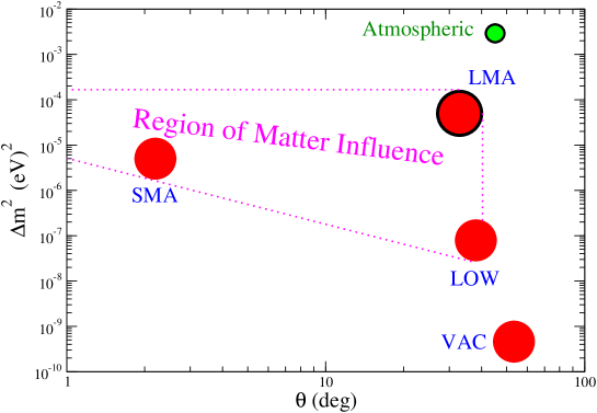
Figure 5: Various solutions to the solar neutrino which were popular prior to SNO’s 2002 papers, plotted in $\Delta m^{2}-\theta$ space. The vacuum (VAC), “low” (LOW) and small mixing angle (SMA) solutions are now thought much less likely than the large mixing angle (LMA) solution. The region where matter effects come into play is shown, as is the solution to the atmospheric neutrino problem, for comparison.

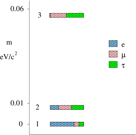
Figure 6: The flavour composition of mass eigenstates assuming the LMA solution for solar neutrino oscillation. The electron component of $\nu_{3}$ is not confirmed and may be very small. The mass scale assumes that $m_{1}$ is zero, which may not be the case. The smaller mass difference may be 2-3 rather than 1-2.

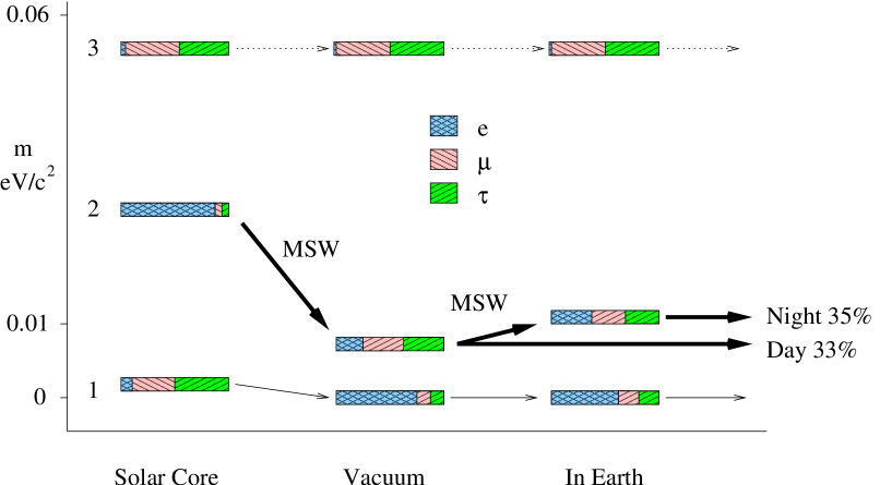
Figure 7: A cartoon of the LMA solution for solar neutrino oscillation. Here is the big picture of solar neutrino physics - including what we know about atmospheric neutrinos - in terms of mass eigenstates and their flavour components. Representing the flavour components as fixed fractions is only really useful here because the oscillations are washed out due to the source size. I assume non-inverted hierarchy and $m_{1}=0$. At the moment there is no evidence for the electron component in $\nu_{3}$; shown here is roughly the maximum possible value. The electron component of $\nu_{1}$ and the non-electron component of $\nu_{2}$ are likely very small. I have also exaggerated the regeneration of $\nu_{e}$ in the earth; the effect may be very tiny.

The solar results were confirmed in December 2002 by the Japanese ultralong-baseline reactor experiment KamLANDkamland . Here we have a point source, and it is therefore OK to revert to thinking of vacuum oscillations. A look at fig.2 shows why all previous reactor experiments with shorter baselines saw no effect, while KamLAND sees 60% of the unoscillated flux at 180 km. Note that the difficulty of these experiments increases rapidly with distance, because even without oscillations, the inverse-square law is in effect, and one rapidly ends up with no signal at all.

VI Big Questions

VI.1 Why don’t charged electrons and muons oscillate?

Electrons, muons (and taus) are charged. The things that we know oscillate ($K^{0}$s, neutrinos) are neutrals. We know two things about neutrals: we can deduce that they were made (by observing other reaction products), and we can deduce that they died (by decay or absorption products). What goes on in between is anyone’s guess (i.e. quantum mechanics). You can figure out that you just made an electron neutrino, and somewhere down the beam pipe figure out that a muon neutrino just interacted and died. The electron and muon neutrino do not have well defined masses (they are not mass eigenstates), but the mass splittings are tiny, so whatever oscillation occurs, we never have to worry about mismatches in measured energies or momentalowe . In between life and death, however, they travel as mass eigenstates ($\nu_{1,2,3}$ )

Charged particles are different, we can track them every mm of the way through a drift chamber. Like Schrödinger’s cat, they interact too much with the environment to be in an ill-defined state. In addition the mass differences are huge (at least 100 MeV, a billion times the biggest neutrino mass difference), so if you watch a muon suddenly become an electron for a few metres and then revert to a muon, there would be major accounting difficulties on the energy/momentum front. For muons and electrons, the mass eigenstates and flavour eigenstates are (have to be?) one and the same thing.

VI.2 Why are the mixings so large?

We don’t know. A clue will come when we measure the electron component in $\nu_{3}$ at Japanese Hadron Facility in the next decadejhf . This angle may be merely small, or tiny enough to be a clue to some new physics. This will also tell us whether the $\nu_{\mu}-\nu_{\tau}$ mixing is actually, or merely approximately, maximal. This will tell us whether the angles are somehow randomly chosen or in some way “special”.

VI.3 If neutrinos exit the Sun without interaction, how does the density of the solar core affect them at all?

This one is the hardest to explain to the man at the bus stop. Its all to do with amplitudes and probabilities. Probabilities (of interaction, say) tend to be the squares of quantum mechanical amplitudes. A solar neutrino can pass through a light year of lead with only a small chance of interaction, so the probability here is tiny. But the amplitude (its square root) is not that small. The way the electron density in the solar core affects neutrinos depends, however, on amplitudes. Hence is it possible to alter the neutrino states while the probability of interaction is negligibly small. The characteristic distance required for this skewing of neutrino states is only about 100 km in the core of the Sun, and a few 1000s of km in the Earthbahcall_book . This is one reason why the day-night asymmetry, if it can be measured at all, is very small. The Sun never dips too far below the horizon even at the most southerly solar neutrino detector (SuperKamiokande, 36^∘ N).

VI.4 What are the absolute masses of the neutrinos?

We’re closing in on this question. We have the splittings, and they are plotted as a function of $m_{1}$ in fig.8. The minimum value $m_{3}$ can have is about 0.06 eV/c². Observation of ripples in the cosmic microwave backgroundWMAP and double-beta decay experimentsvogel set the maximum to be about 0.2 eV/c². Another decade of hard work should close this gap.

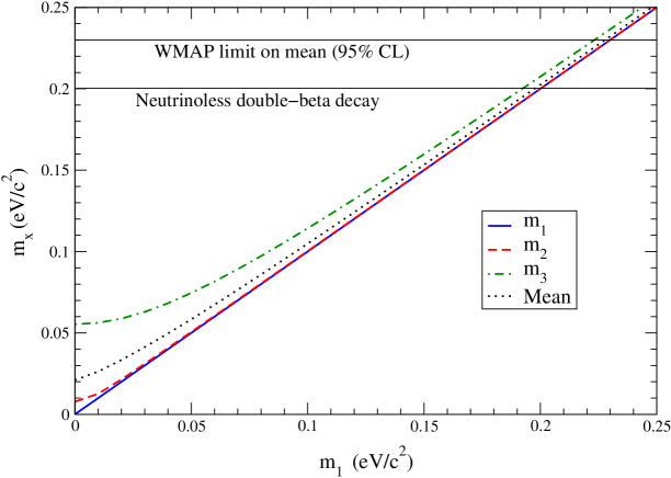
Figure 8: Merging neutrino oscillation evidence with absolute mass limits from measurements of the cosmic microwave background and double-beta decay. The masses $m_{1,2,3}$ are plotted for varying values of $m_{1}$, from zero up to the absolute mass limit.

VI.5 What is the mass of an electron (or mu or tau) neutrino?

The $\nu_{e}$ doesn’t have a well-defined mass; it is a thorough mix of two (or three) neutrinos states which do have well-defined, but different masses. If evidence of a neutrino mass is seen in $\beta$-decay spectra, it will be an averaged value (depending on the mixing angles) of these mass eigenstates.

VI.6 Will we be able to see the decay $\mu\rightarrow e\gamma$?

No. By the tenets of the Uncertainty Principle one can, for a very short period of time, turn a muon into a heavy $W$ and a $\nu_{\mu}$ (fig.9). This $\nu_{\mu}$ can in principle oscillate into a $\nu_{e}$, which can coalesce with the $W$ into an electron. The $\gamma$-ray carries away the excess energy and momentum and everyone is happy. However, Heisenberg tells us we can borrow 80 GeV for a $W$ for only 10^-26s or so. But we already know that it takes 1000s of km for a 100 MeV (the muon’s mass) neutrino to oscillate. That’s many milliseconds (an eternity) at the speed of light, so its never going to happen.

Figure 9: Feynman diagram for $\mu\rightarrow e\gamma$. Imagine time running left to right. The heavy $W^{+}$ can link a muon with a muon neutrino, or an electron with an electron neutrino, and also - because it is charged - shake off a gamma ray. Hence if the neutrinos mix, so must the muon and electron. However, the big mass-energy of the $W^{+}$ can only be borrowed for a brief $10^{-26}$s, too short for the leisurely neutrino oscillation to take place.

VII A Musical Analogy

Consider two adjacent piano strings, tuned to very nearly the same pitch, ($\omega_{1}$, $\omega_{2}$) attached to the sound board. Pluck or strike one string, and soon both strings will be oscillating with a mixture of the two modes, one with the strings in phase, one with them in antiphase. The frequencies of these modes are $\Omega_{+}$ and $\Omega_{-}$, as shown in fig.10. The secret of the piano sound is that the $\Omega_{+}$ mode couples very strongly to the sound board and makes a loud but rapidly decaying sound. The $\Omega_{-}$ mode couples only weakly to the sound board (the motion of one string negates the other) and produces a soft but sustained soundweinreich .

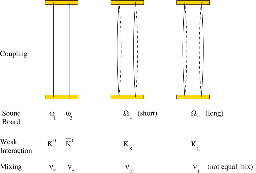
Figure 10: The analogy between piano strings, neutral kaons, and vacuum oscillations. That for neutral kaons is rather exquisite, but for neutrinos one has to remember that the mixture of $e$ and $x=\mu-\tau$ in $\nu_{1,2}$ is not equal but in the ratio $\frac{1}{4}$::$\frac{3}{4}$.

This is a useful approximate analogy for neutrino vacuum oscillations. Each string can be considered a flavour eigenstate, but the time development goes on in terms of the $\Omega_{\pm}$ modes. Averaged over time, half the energy appears in each string, regardless of which string is struck. However, the neutrino mixing is not 50-50 (at least not for solar neutrinos), and neutrinos do not decay, as does a sounding string.

As an aside, this is a much more elegant analogy of the other significant oscillation phenomenon in particle physics, that of neutral kaons. These are made as flavour eigenstates $K^{0}$ and $\bar{K}^{0}$, but these are not mass eigenstates (just like neutrinos). Whichever one you make, it propagates as mix ($K^{0}+\bar{K}^{0}$ or $K^{0}-\bar{K}^{0}$) of two states which have radically different decay times (called “K-long” and “K-short”). One can even, in the string analogy, regenerate the rapidly decaying component by damping one string, in the same manner as one regenerates K-short particles by placing a thin piece of material in the beam, thus preferentially “damping-out” the $K^{0}$s.

However, if one now considers a sound board to have a characteristic frequency $\omega_{B}$ and two identical string with frequency $\omega_{S}$, then one finds that the resonant frequencies of the whole system $\Omega_{\pm}$ behave as shown in fig.11gough .

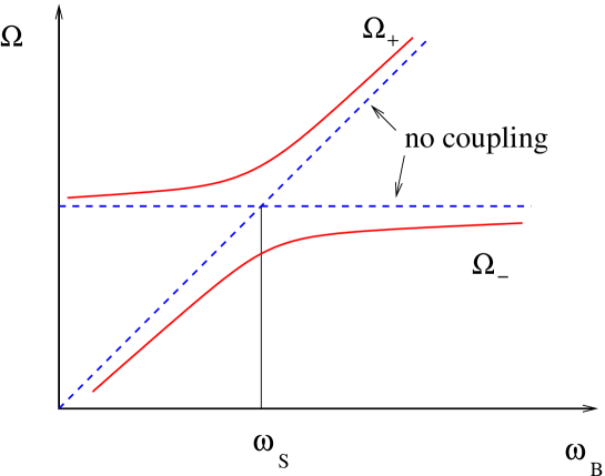
Figure 11: Resonant frequencies $\Omega_{\pm}$ of a system consisting of a sound board with a characteristic frequency $\omega_{B}$ and two identical strings with frequency $\omega_{S}$. The dashed line shows the case where there is no coupling between string and sound board.

With no coupling one has two frequencies $\omega_{B}$ and $\omega_{S}$. With coupling the same is true so long as $\omega_{B}$ is either much higher or much lower than $\omega_{S}$. The interesting part occurs when the two frequencies are very similar, and this is an analogy with what happens when $\nu_{2}$ are born and travel out from the solar core. At birth in the dense core, $m_{2}$ is dictated by fundamental physics and the electron density (i.e. the sound board frequency “$\omega_{B}$”). As it leaves the Sun, this state passes through the resonance region and emerges as the higher of the two mass states (“$\Omega_{+}$”), the one with 25% electron content.

Incidentally, the SMA solution involved a rapid (“non-adiabatic”) passage through the resonance region which allowed a hop from the $\Omega_{+}$ to $\Omega_{-}$ states, even with a tiny coupling. As we have seen, however, nature did not go this route.

VIII Conclusion

In neutrinos we are confronted by real particles which behave in a quantum mechanical fashion over very large distances, 1000s of km. We are not used to this, and the physics community has yet to assimilate fully the implications.

References

-
(1)
K.Nakamura, “Solar
Neutrinos”, in the 2002 Review of Particle Properties,
http://pdg.lbl.gov/2002/solarnu_s005313.pdf -
(2)
Particle Data Group
http://pdg.lbl.gov/ -
(3)
John Bahcall homepage
http://www.sns.ias.edu/~jnb/ - (4) R. Davis Jr., D. S. Harmer and K. C. Hoffman, Phys. Rev. Lett. 20 (1968) 1205.
-
(5)
www.nobel.se/physics/laureates/2002/ - (6) A. I. Abasov et al., Phys. Rev. Lett. 67 (1991) 3332.
- (7) P. Anselmann et al., Phys. Lett. B285 (1992) 376.
-
(8)
C. E. Waltham, Physics in Canada 49
(1993) 81-86 and 356-357, and
http://xxx.lanl.gov/abs/physics/0206076 -
(9)
SNO homepage
http://www.sno.phy.queensu.ca/ - (10) V. N. Gribov and B. M. Pontecorvo, Phys. Lett. B28 (1969) 493.
- (11) K. S. Hirata et al., Phys. Rev. Lett. 63 (1989) 16.
- (12) K. S. Hirata et al., Phys. Lett. B280 (1992) 146.
-
(13)
SuperKamiokande
homepage
http://www-sk.icrr.u-tokyo.ac.jp/sk/ - (14) Q. R. Ahmad et al., Phys. Rev. Lett. 89 (2002) 011301 and 011302.
-
(15)
Y. Itow et al.,
http://xxx.lanl.gov/abs/hep-ex/0106019 - (16) N. Jelley, priv. comm., and M. G. Bowler, SNO internal report (2002).
-
(17)
B. Kayser
“Neutrino Physics as Explored by Flavor Change”, in the 2002 Review of
Particle Properties,
http://pdg.lbl.gov/2002/neutrino_mixing_s805.pdf -
(18)
KamLAND homepage
http://kamland.lbl.gov/ -
(19)
H. Burkhardt,
J. Lowe, G. J. Stephenson
Jr. and T. Goldman,
http://xxx.lanl.gov/abs/hep-ph/0302084 - (20) J. Bahcall, “Neutrino Astrophysics” (Cambridge, 1989).
-
(21)
Wilkinson
Microwave Anisotropy Probe
(WMAP) homepage
http://map.gsfc.nasa.gov/m_mm.html -
(22)
P.Vogel
“Limits from Neutrinoless Double-Beta Decay”, in the 2002 Review of
Particle Properties,
http://pdg.lbl.gov/2002/betabeta_s076.pdf -
(23)
G. Weinreich, J. Acoust. Soc. Am. 62
(1977) 1474,
http://www.speech.kth.se/music/5_lectures/weinreic/weinreic.html#top - (24) C. E. Gough, Acustica 49 (1981) 124.