A Method for Ultrashort Electron Pulse Shape-Measurement Using Coherent Synchrotron Radiation

Abstract

In this paper we discuss a method for nondestructive measurements of the longitudinal profile of sub-picosecond electron bunches for X-Ray Free Electron Lasers (XFELs). The method is based on the detection of the Coherent Synchrotron Radiation (CSR) spectrum produced by a bunch passing a dipole magnet system. This work also contains a systematic treatment of synchrotron radiation theory which lies at the basis of CSR. Standard theory of synchrotron radiation uses several approximations whose applicability limits are often forgotten: here we present a systematic discussion about these assumptions. Properties of coherent synchrotron radiation from an electron moving along an arc of a circle are then derived and discussed. We describe also an effective and practical diagnostic technique based on the utilization of an electromagnetic undulator to record the energy of the coherent radiation pulse into the central cone. This measurement must be repeated many times with different undulator resonant frequencies in order to reconstruct the modulus of the bunch form-factor. The retrieval of the bunch profile function from these data is performed by means of deconvolution techniques: for the present work we take advantage of a constrained deconvolution method. We illustrate with numerical examples the potential of the proposed method for electron beam diagnostics at the TESLA Test Facility (TTF) accelerator. Here we choose, for emphasis, experiments aimed at the measure of the strongly non-Gaussian electron bunch profile in the TTF femtosecond-mode operation. We demonstrate that a tandem combination of a picosecond streak camera and a CSR spectrometer can be used to extract shape information from electron bunches with a narrow leading peak and a long tail.

DEUTSCHES ELEKTRONEN-SYNCHROTRON

DESY 03-031

March 2002

1 Introduction

Electron bunches with very small transverse emittance and high peak current are needed for the operation of XFELs [1, 2]. This is achieved using a two-step strategy: first generate beams with small transverse emittance using an RF photocathode and, second, apply longitudinal compression at high energy using a magnetic chicane. The bunch length for XFEL applications is of order of 100 femtoseconds. Since detailed understanding of longitudinal dynamics in this new domain of accelerator physics is of paramount importance for FEL performance, experiments on this subject are planned in test facilities. The femtosecond time scale is beyond the range of standard electronic display instrumentation and the development of nondestructive methods for the measurement of the longitudinal beam current distribution in such short bunches is undoubtedly a challenging problem: in this paper we discuss one of these methods, which is based on spectral measurements of Coherent Synchrotron Radiation (CSR) produced by a bunch passing a dipole magnet or an undulator.

After the compression stage, the CSR pulse can be analyzed, for example, with a spectrometer. As we point out in Section 2, we can decompose the coherent radiation spectrum, $P(\omega)$, into the product of the square modulus of the bunch form factor, $\mid\bar{F}(\omega)\mid^{2}$, and the single particle radiation spectrum, $p(\omega)$ [3]. The CSR spectrum, then, provides information on the bunch form factor, although one has to keep in mind that, in order to find $\mid\bar{F}(\omega)\mid^{2}$ from $P(\omega)$, one needs the quantity $p(\omega)$.

Section 3 contains a systematic treatment of synchrotron radiation theory. All the results presented in this section are derived from fundamental laws of electrodynamics and the reader can follow the whole derivation process from beginning to end. We use a synthetic approach to present the material: simple situations are studied first, and more complicated ones are introduced gradually. Previous experience in synchrotron radiation theory would be helpful but is not absolutely necessary, because all the required material is independently derived. In this respect our paper is reasonably self-contained.

A clear message in this work is that reexamination of dogmatic ”truths” can sometimes yield surprises. For years we were led to believe that famous Schwinger’s formulas [4] are directly applicable to the case of synchrotron radiation from dipole magnet and even now no attention is usually paid to the region of applicability of these expressions. While such formulas are valid in order to describe radiation from a dipole in the X-ray range, their long wavelength asymptotic are not valid, in general. Analytical study of this matter was first performed in the 80’s [5]. However, standard texts on synchrotron radiation theory do not seem to provide a derivation of the expression for the synchrotron radiation from an electron moving along an arc of a circle. In Section 3 we present such a derivation, which we believe is quite simple and instructive. Properties of coherent synchrotron radiation from dipole magnets in the time domain are derived and discussed too.

Standard theory of synchrotron radiation relies upon other approximations too, and it seems interesting to pay attention to their region of applicability. To be specific, two important limitations are discussed. First, it is usually assumed that the observer lies at infinite distance from the source. Second, people don’t pay attention to the fact that, in real experimental conditions, the radiation is seen by the detector through some limited aperture. Thus, both finite distance effects and diffraction effects are ignored. The aperture sizes and the distances for which the latter assumptions are valid are so large, in long wavelength range, as to be of limited practical interest. We can draw at least two main conclusions from Section 3: first, long wavelength radiation spectrum distortions can arise, physically, from violation of the far zone assumption or from aperture limitations (or both). Second, a CSR diagnostic method based on the famous Schwinger’s formulas (or the ones derived in [5]) is of purely theoretical interest. In real accelerators, the long wavelength synchrotron radiation from bending magnet in the near zone integrates over many different vacuum chamber pieces with widely varying aperture and $p(\omega)$ is usually a very difficult quantity to calculate with great accuracy.

An effective and practical technique based on the spectral properties of undulator radiation can be used to characterize the bunch profile function. The method we describe in Section 4 uses an electromagnetic undulator and it is based on recording the energy of coherent radiation pulses in the central cone. This coherent radiation energy turns out to be proportional, per pulse, to the square modulus of the bunch form-factor at the resonant frequency of the fundamental harmonic. The measurement must be repeated many times with different undulator resonant frequencies (which are tuned by changing the undulator parameters) in order to reconstruct the modulus of the bunch form-factor.

The retrieval of the bunch profile function from the modulus of its form factor is preformed, in Section 5, by means of a deconvolution technique. For the present work we choose a constrained deconvolution method. This consists in finding the best estimate of the bunch profile function, $F(t)$, for a particularly measured form-factor modulus, $\mid\bar{F}(\omega)\mid$, including utilization of any a priori available information about $F(t)$. In the end of the paper we illustrate with a numerical example the potential of the proposed technique for diagnostics at the TESLA Test Facility accelerator. Here we have chosen, for emphasis, an experiment aimed at measuring the strongly non-Gaussian electron bunch profile at TTF, Phase 2 in femtosecond mode operation. The femtosecond mode operation is based on the experience obtained during the operation of the TTF FEL, Phase 1 [6] and it requires one bunch compressor only. An electron bunch with a sharp spike at the head is prepared with an rms width of about 20 microns and a peak current of about one kA. This spike in the bunch generates FEL pulses with duration below one hundred femtoseconds. We demonstrate that a tandem combination of a picosecond streak camera and CSR spectrometer can be used to extract shape information from electron bunches with a narrow leading peak and a long tail.

2 Physics of coherent synchrotron radiation

To begin our consideration, let us recall some well-known aspects of CSR. From a microscopic viewpoint, the electron beam current at the entrance of a bending magnet is made up of moving electrons arriving randomly at the entrance of the bending magnet:

$$J(t)=(-e)\sum^{N}_{k=1}\delta(t-t_{k})\ ,$$

where $\delta(\cdot)$ is the delta function, $(-e)$ is the (negative) electron charge, $N$ is the number of electrons in a bunch and $t_{k}$ is the random arrival time of the electron at the bending magnet entrance. The electron bunch profile is described by the profile function $F(t)$. The beam current averaged over an ensemble of bunches can be written in the form:

$$\langle J(t)\rangle=(-e)NF(t)\ .$$

The profile function for an electron beam with Gaussian current distribution is given by:

$$F(t)=\frac{1}{\sqrt{2\pi}\sigma_{\mathrm{T}}}\exp\left(-\frac{t^{2}}{2\sigma^{2}_{\mathrm{T}}}\right)\ .$$

and the probability of arrival of an electron during the time interval $(t,t+\mathop{\mathrm{d}}t)$ is just equal to $F(t)\mathop{\mathrm{d}}t$.

The electron beam current, $J(t)$, and its Fourier transform, $\bar{J}(\omega)$, are connected by

$$\bar{J}(\omega)=\int\limits^{\infty}_{-\infty}\exp(\mathop{\mathrm{i}}\omega t)J(t)\mathop{\mathrm{d}}t=(-e)\sum^{N}_{k=1}\exp(\mathop{\mathrm{i}}\omega t_{k})\ ,$$

$$J(t)=\frac{1}{2\pi}\int\limits^{\infty}_{-\infty}\exp(-\mathop{\mathrm{i}}\omega t)\bar{J}(\omega)\mathop{\mathrm{d}}\omega=(-e)\sum^{N}_{k=1}\delta(t-t_{k})\$$

and, therefore, the average value of $\mid\bar{J}(\omega)\mid^{2}$ can be written as:

$$\langle\bar{J}(\omega)\bar{J}^{*}(\omega)\rangle=e^{2}N+e^{2}\sum_{k\neq n}\langle\exp(\mathop{\mathrm{i}}\omega t_{k})\rangle\langle\exp(-\mathop{\mathrm{i}}\omega t_{n})\rangle\ .$$

The expression $\langle\exp(\mathop{\mathrm{i}}\omega t_{k})\rangle$ is nothing but the Fourier transform of the bunch profile function $F(t)$, since:

$$\langle\exp(\mathop{\mathrm{i}}\omega t_{k})\rangle=\int\limits^{\infty}_{-\infty}F(t_{k})\exp(\mathop{\mathrm{i}}\omega t_{k})\mathop{\mathrm{d}}t_{k}=\bar{F}(\omega)\ .$$

Thus we can write:

$$\langle\mid\bar{J}(\omega)\mid^{2}\rangle=e^{2}N+e^{2}N(N-1)\mid\bar{F}(\omega)\mid^{2}\ ,$$

where the Fourier transform of the Gaussian profile function has the form:

$$\bar{F}(\omega)=\exp\left(-\frac{\omega^{2}\sigma^{2}_{\mathrm{T}}}{2}\right)\ .$$ (3)

Above we described the properties of the input signal in the frequency domain. The next step is the derivation of the spectral function connecting the Fourier amplitudes of the output field and the Fourier amplitudes of the input signal. We will investigate the synchrotron radiation in the framework of a one-dimensional model. Also, we will assume that the cross section of the particle beam is small compared with the distance to the observer, so that the path length difference from any point of the beam cross section to the observer are small compared to the shortest wavelength involved.

The component of synchrotron radiation electric field in time domain, $E_{x,y}(t)$, and its Fourier transform, $\bar{E}_{x,y}(\omega)$, are connected by

$$E_{x,y}(t)=\frac{1}{2\pi}\int\limits^{\infty}_{-\infty}\bar{E}_{x,y}(\omega)\exp(-\mathop{\mathrm{i}}\omega t)\mathop{\mathrm{d}}\omega\ ,$$

and the Fourier harmonic for $\omega<0$ is defined by the relation $\bar{E}^{*}(\omega)=\bar{E}(-\omega)$. On the other hand, the Fourier harmonic of the electromagnetic field and the Fourier harmonic of the current at the dipole magnet entrance are connected by:

$$\bar{E}_{x,y}(\omega)=A_{x,y}(\omega)\bar{J}(\omega)\ ,\quad\omega>0\ ,$$

where $A_{x,y}(\omega)$ is the synchrotron radiation spectral function of the dipole. Since the radiation power is proportional to the square of the radiation field, the averaged total power at a certain frequency $\omega$ is given by the expression:

$$P(\omega)=p(\omega)[N+N(N-1)\mid\bar{F}(\omega)\mid^{2}]\ ,$$ (4)

where $p(\omega)$ is the radiation power from one electron. The first term $N$ in square bracket represents ordinary incoherent synchrotron radiation with a power proportional to the number of radiating particles. The second term represents coherent synchrotron radiation. The actual coherent radiation power spectrum depends on the particular particle distribution in the bunch. For photon wavelengths equal and longer than the bunch length, we expect all particles within a bunch to radiate coherently and the intensity to be proportional to the square of the number of $N$ of particles rather than linearly proportional to $N$, as in the usual incoherent case. This quadratic effect can greatly enhance the radiation since the bunch population can be from $10^{8}$ to $10^{11}$ electrons. On the other hand the coherent radiation power falls off rapidly for wavelengths as short or even shorter than the rms bunch length.

A method for estimating the bunch profile function $F(t)$ is to compute the factor $p(\omega)$, to measure the CSR power spectrum $P(\omega)$ and to deduce the factor $\mid\bar{F}(\omega)\mid^{2}$ from equation (4). However, it is clear that the retrievable information about the profile function will, in general, not be complete, for it is the particular measured square modulus of the form-factor that can be obtained, not the complex form-factor itself.

3 Radiation from dipole magnet

The phenomenon of coherent synchrotron radiation has been introduced in a conceptual way in the preceding section. As was pointed out, the CSR power spectrum is the product of the square modulus of bunch form-factor $\mid\bar{F}(\omega)\mid^{2}$, and the single-particle power spectrum $p(\omega)$. Any diagnostics method based on CSR must devote therefore attention to correctly determinate the synchrotron radiation spectrum from one electron $p(\omega)$, for this quantity plays a critical role in the form-factor measurement. In the present section we will deal with the properties of the single-particle radiation in time and in frequency domain as well as with the CSR properties in time domain. In order to give the subject a semblance of continuity, it will be desirable to introduce considerable matter which can be found in any of standard text on synchrotron radiation theory (see for example [3],[7],[8]). The typical textbook treatment consists in finding the expression for the synchrotron radiation spectrum from an electron moving in a circle. However, no attention is usually paid to the region of applicability of the derived expressions. For instance, the standard extension of the theory to the case of synchrotron radiation from dipole magnet is based on the assumption that the energy spectrum formula is equivalent to the famous Schwinger’s formula [4]. While this formula is valid for the X-ray range, it does not provide a satisfactory description in the long wavelength asymptotic [5]. Moreover Scwinger’s formulas are found in the limit of an infinite observer distance and under the approximation of no limiting aperture through which the radiation is collected. Here we pay particular attention to the region of applicability of Schwinger’s formulas; specifically, we derive expressions for the time and frequency dependence of the electromagnetic radiation produced by an electron moving along an arc of a circle, and we investigate how the CSR field pulse in the time domain is modified in more realistic situations.

3.1 Radiation field in the time domain

Figure 1: Geometry for synchrotron radiation production from a bending magnet

Figure 2: Synchrotron radiation production from circular motion. Directions of acceleration vector as seen by an observer at $P$, drawn in plane view

Figure 3: Time variation of a synchrotron radiation pulse generated by a highly relativistic electron moving in a circle as seen by an observer in the orbital plane

Figure 4: Synchrotron radiation production from an arc of a circle. Directions of acceleration vector as seen by an observer at $P$, drawn in plane view

Figure 5: Time variation of a synchrotron radiation pulse generated by a highly relativistic electron moving along an arc of a circle. The normalized bending angle is $\hat{\phi}_{\mathrm{m}}=\gamma\phi_{\mathrm{m}}=2.5$

Figure 6: Time variation of a synchrotron radiation pulse generated by a highly relativistic electron moving along an arc of a circle. The normalized bending angle is $\hat{\phi}_{\mathrm{m}}=\gamma\phi_{\mathrm{m}}=1.5$

Figure 7: Time variation of a synchrotron radiation pulse from a short bending magnet. The normalized bending angle is $\hat{\phi}_{\mathrm{m}}=\gamma\phi_{\mathrm{m}}=0.5$

Let us start reviewing how a single electron radiates as it moves in a dipole magnet. The electron is subjected to an acceleration, $\dot{\vec{v}}=c\dot{\vec{\beta}}$, of magnitude $c^{2}\beta^{2}/R$ so that a distant observer detects the electric and magnetic fields in the form of electromagnetic waves from the radiating electron. Fig. 1 shows the relationship between the observer at a fixed point $P$, whose coordinates are $(\vec{r}_{0},t)$, and the radiating electron at $(\vec{R},t^{\prime})$, $t^{\prime}$ being the emission (or retarded) time. The fundamental laws of electrodynamics tell that the electric field of a charge $(-e)$ moving along an arbitrary trajectory is given by the Lienard-Wiechert formula

$$\vec{E}(t)=\frac{(-e)}{\mid\vec{r}\mid^{2}}\frac{1}{\gamma^{2}}\left[\frac{(\vec{n}-\vec{\beta})}{(1-\vec{n}\cdot\vec{\beta})^{3}}\right]_{\mathrm{r}}+\frac{(-e)}{c\mid\vec{r}\mid}\left[\frac{\vec{n}\times[(\vec{n}-\vec{\beta})\times\dot{\vec{\beta}}]}{(1-\vec{n}\cdot\vec{\beta})^{3}}\right]_{\mathrm{r}}\ ,$$

where $\vec{n}$ is a unit vector along the line from the point at which the radiation is emitted at the emission time to the observation point at the observation time, and we understand that the quantity in brackets must be evaluated at the retarded time $t^{\prime}=t-\frac{1}{c}\mid\vec{r}(t^{\prime})\mid$. The latter equation consists of two distinct parts. The first is inversely proportional to the square of the distance between radiation source and observer, depends only on the charge velocity and is known as velocity or Coulomb field. The second is inversely proportional to the distance from the charge, depends also on the charge acceleration and it is known as acceleration or radiation field. At large distances from the moving electron, the acceleration-related term dominates, and it is usually associated to the electromagnetic radiation of the charge. The region of space where the radiation field dominates is called a far (or wave) zone and the radiative electric field in the far zone is given by the formula

$$\vec{E}_{\mathrm{r}}(t)=\frac{(-e)}{c\mid\vec{r}_{0}\mid}\left[\frac{\vec{n}\times[(\vec{n}-\vec{\beta})\times\dot{\vec{\beta}}]}{(1-\vec{n}\cdot\vec{\beta})^{3}}\right]_{\mathrm{r}}\ .$$ (5)

We can use (5) to look at all kinds of interesting problems. This is a complicated expression, but it is easy enough to be used in a computer calculation which can be further visualized as a geometrical picture. Such geometrical pictures will give us a good qualitative description of the situation. Usual theory of synchrotron radiation is based on the assumption that the electron is moving on a circle and radiation is observed from the whole circular trajectory, so that in each cycle we get a sharp pulse of electric field. A far-field computation of the predicted time dependence of synchrotron radiation for circular motion is presented in Fig. 3. The horizontal component of electric field plotted versus the normalized variable $\omega_{\mathrm{c}}t$, where $\omega_{\mathrm{c}}=3\gamma^{3}c/(2R)$ is the critical frequency of synchrotron radiation. The field in the orbital plane has a zero around $t=\omega_{\mathrm{c}}^{-1}$. Numerically from Fig. 3 one obtains

$$\int\limits^{\infty}_{-\infty}\vec{E}_{\mathrm{r}}\mathop{\mathrm{d}}t=0\ .$$ (6)

It is interesting to stress the fact that equation (6) is strictly related to the well-known result that a uniformly charged ring does not radiate. In fact, starting from (6) one can show that a system of $N$ identical equidistant charges $(-e)$ moving with constant velocity $v$ along a circle does not radiate in the limit for $N\to\infty$ and $(-e)N={\mathrm{const}}$, and the electric and the magnetic fields of the system are the usual static values.

Figure 8: Geometry for an infinite uniform current progressing through an arc of a circle and relative position of an observer

It is important to realize that (6) is valid only when the electron is moving in a circle. But we now want to study synchrotron radiation from an electron moving along the arc of a circle (see Fig. 4). By inspecting Fig. 5 - 7, one can see that when the electron moves in arcs of circles with different angular extensions $\phi_{m}$, the time-average of the electric field is nonzero.

Let us consider for a moment (in parallel with what has been done in the case of a circle) the case of infinitely long electron bunch with the homogeneous linear density $\lambda_{0}$ and current $I=-ev\lambda_{0}$. A current circuit consists of the arc and semi-infinite straight lines (see Fig. 8). The angle between the straight lines is equal to the bending angle $\phi_{\mathrm{m}}$ of the magnet. The fact that the average electric field from a single particle is different from zero means that the acceleration field from our infinite circuit must be different from zero too. Then we have deal with an intriguing paradox, since it is a well known result that an uniform electron current does not radiate, not only in the case of circular motion, but independently from the trajectory .

It is possible to explain this contradiction in very simple terms as follows. First of all we know that the velocity (electric) field from a line current (including our case) is proportional to $1/\mid\vec{r}_{\perp}\mid$, where $\mid\vec{r}_{\perp}\mid$ is the distance of the observer from the line charge. Second, in our case, the acceleration part of the electric field is proportional to $1/\mid\vec{r}\mid$, where $\mid\vec{r}\mid$ is the distance of the observer from the magnet (since the acceleration field sources are strictly limited to the particles in the magnet only). The situation is depicted in Fig. 8: the ratio $\mid\vec{r}_{\perp}\mid/\mid\vec{r}\mid$ is finite for any position of observer therefore there is no region in space where the acceleration field dominates. This last observation solves our paradox since, in the case of infinite charge current in an arc of a circle, we cannot talk about far zone at all, although a non-zero acceleration field is present.

It is interesting to discuss, at this point, the shape of the coherent synchrotron radiation field pulse under different trajectories. What we have been dealing with before is simply a far field analysis of the single-particle radiation field. When a large number of electrons move together, all the same way, the total field will be a linear superposition of the individual particle fields. Of course the result depends upon the longitudinal distribution of the electrons. One aspect of the problem that we can immediately deal with is the coherent synchrotron radiation production from a ”short” magnet, i.e. $\phi_{m}\ll 1/\gamma$. We can assert that the field appears as shown in Fig. 9. In fact the time-dependence of the field has, for every electron, the shape shown in Fig. 7 and the total field emitted by the electron bunch is represented by a sum of these pulses, one for each radiating electron. In the limit for ”short” magnets, the reader can easily come to the intuitive conclusion that the time profile of the electron bunch density is linearly encoded onto the electric field of the radiation pulse. The width of the temporal profile of the electric field corresponds directly to the electron bunch length, and the shape of the temporal profile is proportional to the longitudinal bunch distribution.

Figure 9: Coherent synchrotron radiation production from a ”short” magnet. The time profile of the electron bunch density is linearly encoded onto the electric field of the radiation pulse. Spikes correspond to spontaneous radiation, and average value of electric field corresponds to CSR. The width of the temporal profile of the electric field corresponds directly to the electron bunch length, and the shape of the temporal profile is proportional to the longitudinal distribution within the bunch

We have just argued that the bunch density is linear encoded onto the electric field as in Fig. 9; nevertheless, in Fig. 9, we illustrate small fluctuations which occur in the field amplitude too. The reason for this is that the electron bunch is composed of large number of electrons, thus fluctuations always exist in the electron beam density due to shot noise effects. For any synchrotron radiation beam there is some characteristic time, which determines the time scale of the random field fluctuations. This characteristic time is called coherence time $\tau_{\mathrm{c}}$ of synchrotron radiation and its magnitude is of the order of the pulse duration from one electron. The physical significance of these fluctuations is that there is a short wavelength radiation component of the radiation in the range of the inverse pulse duration from a single electron. Simple physical considerations show that the energy spectrum of this hard radiation component is order of $P(\omega)\simeq Np(\omega)$. This explains the relation between small fluctuations of the radiation field amplitude and spontaneous (incoherent) emission of synchrotron radiation.

Up to this point we only talked about coherent radiation from a ”short” magnet. Ultimately we want to consider CSR production from an arc of a circle. An easier step in this direction consists in the analysis of the CSR time pulse from a circular motion. It is possible, indeed, to derive a simple analytical expression for the CSR pulse from a bunch with an arbitrary distribution of the linear density satisfying the following condition:

$$\frac{R}{c\gamma^{3}}\frac{\mathop{\mathrm{d}}F(t)}{\mathop{\mathrm{d}}t}\ll F(t)\ .$$ (7)

The latter condition simply indicates that the characteristic length of the bunch is much larger than $R/\gamma^{3}$. Let us express the total CSR pulse as a superposition of single particle fields at a given position in the far zone:

$$\vec{E}_{\mathrm{CSR}}(t)=\int\limits^{\infty}_{-\infty}\vec{E}_{\mathrm{r}}(t-\tau)NF(\tau)\mathop{\mathrm{d}}\tau\ ,$$ (8)

where we calibrated the observer time in such a way that, when $F(\tau)=\delta(\tau)$, the single particle radiation pulse has its maximum at $t=0$. To calculate the integral in (8) one should take into account the property (6) of the kernel $\vec{E}_{\mathrm{r}}(t-\tau)$ which has been discussed above. Using (6) and (7) one can simplify equation (8) in the following way. The integral (8) is written down as a sum of three integrals

$$\vec{E}_{\mathrm{CSR}}(t)=\int\limits^{t-\delta_{1}}_{-\infty}\vec{E}_{\mathrm{r}}(t-\tau)NF(\tau)\mathop{\mathrm{d}}\tau$$

$$+\int\limits^{t+\delta_{2}}_{t-\delta_{1}}\vec{E}_{\mathrm{r}}(t-\tau)NF(\tau)\mathop{\mathrm{d}}\tau+\int\limits^{\infty}_{t+\delta_{2}}\vec{E}_{\mathrm{r}}(t-\tau)NF(\tau)\mathop{\mathrm{d}}\tau\ ,$$ (9)

where $\delta_{(1,2)}$ satisfy the following conditions:

$$\delta_{(1,2)}\gg\frac{R}{c\gamma^{3}}\ ,\quad\delta_{(1,2)}\frac{\mathop{\mathrm{d}}F(t)}{\mathop{\mathrm{d}}t}\ll F(t)\ .$$ (10)

The bunch profile function is, therefore, a slowly varying function of the time and we simply take $F(\tau)$ outside the integral sign and call it $F(t)$ when calculating the second integral of (9):

$$\int\limits^{t+\delta_{2}}_{t-\delta_{1}}\vec{E}_{\mathrm{r}}(t-\tau)NF(\tau)\mathop{\mathrm{d}}\tau\simeq NF(t)\int\limits^{t+\delta_{2}}_{t-\delta_{1}}\vec{E}_{\mathrm{r}}(t-\tau)\mathop{\mathrm{d}}\tau\ .$$ (11)

Then we remember that the average of the electric field over time is zero when an electron is moving in a circle. As a result, we rewrite the integral in the form:

$$\int\limits^{t+\delta_{2}}_{t-\delta_{1}}\vec{E}_{\mathrm{r}}(t-\tau)\mathop{\mathrm{d}}\tau=-\left[\int\limits^{t-\delta_{1}}_{-\infty}\vec{E}_{\mathrm{r}}(t-\tau)\mathop{\mathrm{d}}\tau+\int\limits^{\infty}_{t+\delta_{2}}\vec{E}_{\mathrm{r}}(t-\tau)\mathop{\mathrm{d}}\tau\right]\ .$$ (12)

Taking into account (11) and (12), the expression for CSR pulse becomes

$$\vec{E}_{\mathrm{CSR}}(t)=\int\limits^{t-\delta_{1}}_{-\infty}\vec{E}_{\mathrm{r}}(t-\tau)NF(\tau)\mathop{\mathrm{d}}\tau-NF(t)\int\limits^{t-\delta_{1}}_{-\infty}\vec{E}_{\mathrm{r}}(t-\tau)\mathop{\mathrm{d}}\tau$$

$$+\int\limits^{\infty}_{t+\delta_{2}}\vec{E}_{\mathrm{r}}(t-\tau)NF(\tau)\mathop{\mathrm{d}}\tau-NF(t)\int\limits^{\infty}_{t+\delta_{2}}\vec{E}_{\mathrm{r}}(t-\tau)\mathop{\mathrm{d}}\tau\ .$$ (13)

Integrating by parts, the first pair of integrals on the right hand side of (13) can be joined in a single one; the same can be done with the second pair:

$$\vec{E}_{\mathrm{CSR}}(t)=-\int\limits^{t-\delta_{1}}_{-\infty}\Phi\left[\vec{E}_{\mathrm{r}}\right](t-\tau)N\frac{\mathop{\mathrm{d}}F(\tau)}{\mathop{\mathrm{d}}\tau}\mathop{\mathrm{d}}\tau$$

$$-\int\limits^{\infty}_{t+\delta_{2}}\Phi\left[\vec{E}_{\mathrm{r}}\right](t-\tau)N\frac{\mathop{\mathrm{d}}F(\tau)}{\mathop{\mathrm{d}}\tau}\mathop{\mathrm{d}}\tau\ ,$$ (14)

where $\Phi\left[\vec{E}_{\mathrm{r}}\right]$ is a primitive of $\vec{E}_{\mathrm{r}}$. What is left to do now is to evaluate a primitive of the radiation field from one electron.

To calculate the primitive of $\vec{E}_{\mathrm{r}}$ we use (5) and note that the electric field is expressed in terms of quantities at the retarded time $t^{\prime}$. The calculation is simplified if we use the following consideration: since, in general $\mathop{\mathrm{d}}t/\mathop{\mathrm{d}}t^{\prime}=(1-\vec{n}\cdot\vec{\beta})$ and

$$\frac{\mathop{\mathrm{d}}}{\mathop{\mathrm{d}}t^{\prime}}\left[\frac{\vec{n}\times[(\vec{n}\times\vec{\beta})]}{(1-\vec{n}\cdot\vec{\beta})}\right]=\left[\frac{\vec{n}\times[(\vec{n}-\vec{\beta})\times\dot{\vec{\beta}}]}{(1-\vec{n}\cdot\vec{\beta})^{2}}\right]\ ,$$

we also have

$$\frac{\mathop{\mathrm{d}}}{\mathop{\mathrm{d}}t}\left[\frac{\vec{n}\times[(\vec{n}\times\vec{\beta})]}{(1-\vec{n}\cdot\vec{\beta})}\right]=\left[\frac{\vec{n}\times[(\vec{n}-\vec{\beta})\times\dot{\vec{\beta}}]}{(1-\vec{n}\cdot\vec{\beta})^{3}}\right]\ .$$

Thus we can write $\vec{E}_{\mathrm{CSR}}(t)$ as

Figure 10: Geometry for synchrotron radiation from circular motion

$$\vec{E}_{\mathrm{CSR}}(t)=\frac{e}{c\mid\vec{r}_{0}\mid}\int\limits^{t-\delta_{1}}_{-\infty}\left[\frac{\vec{n}\times[(\vec{n}\times\vec{\beta})]}{(1-\vec{n}\cdot\vec{\beta})}\right]_{(t-\tau)}N\frac{\mathop{\mathrm{d}}F(\tau)}{\mathop{\mathrm{d}}\tau}\mathop{\mathrm{d}}\tau$$

$$+\frac{e}{c\mid\vec{r}_{0}\mid}\int\limits^{\infty}_{t+\delta_{2}}\left[\frac{\vec{n}\times[(\vec{n}\times\vec{\beta})]}{(1-\vec{n}\cdot\vec{\beta})}\right]_{(t-\tau)}N\frac{\mathop{\mathrm{d}}F(\tau)}{\mathop{\mathrm{d}}\tau}\mathop{\mathrm{d}}\tau\ ,$$ (15)

where the quantity in brackets must be evaluated at the retarded time $t^{\prime}=(t-\tau)-\frac{1}{c}\mid\vec{r}(t^{\prime})\mid$.

Now we would like to compute the quantities required for (15). Since (10) holds, we can substitute the function in brackets in both integrals on the right hand side of (15) with its asymptotic behavior at $\tau\gg R/(c\gamma^{3})$. Because the angles are very small and the relativistic $\gamma$ factor is very large, it is very useful to express (15) in a small angle approximation. The triple vector product is calculated from Fig. 10

$$\vec{n}\times[\vec{n}\times\vec{\beta}]=\omega_{0}t^{\prime}\vec{e}_{x}+\theta\vec{e}_{y}\ .$$ (16)

Here $\theta$ is the vertical angle, $\omega_{0}=c/R$ is the revolution frequency and $\vec{e}_{x,y}$ are unit vectors directed along the $x$ and $y$ axis of the fixed Cartesian coordinate system $(x,y,z)$ shown in Fig. 10. The definition of $\vec{n}$ and $\vec{R}$ can be used to compute the scalar product in the denominator in (15) so that

$$\vec{n}\cdot\vec{\beta}=\beta\cos\theta\cos\omega_{0}t^{\prime}\simeq\beta(1-\theta^{2}/2)(1-(\omega_{0}t^{\prime})^{2}/2)\ .$$ (17)

We assume, here, that the vertical angle is small enough and we can leave out the cosine factor. We can now write $\vec{E}_{\mathrm{CSR}}(t)$ as

$$\vec{E}_{\mathrm{CSR}}(t)=\frac{2e}{c\mid\vec{r}_{0}\mid}\left\{\int\limits^{t-\delta_{1}}_{-\infty}\left[\frac{\left(\omega_{0}t^{\prime}\vec{e}_{x}+\theta\vec{e}_{y}\right)}{(\omega_{0}t^{\prime})^{2}}\right]_{(t-\tau)}N\frac{\mathop{\mathrm{d}}F(\tau)}{\mathop{\mathrm{d}}\tau}\mathop{\mathrm{d}}\tau\right.$$

$$+\left.\int\limits^{\infty}_{t+\delta_{2}}\left[\frac{\left(\omega_{0}t^{\prime}\vec{e}_{x}+\theta\vec{e}_{y}\right)}{(\omega_{0}t^{\prime})^{2}}\right]_{(t-\tau)}N\frac{\mathop{\mathrm{d}}F(\tau)}{\mathop{\mathrm{d}}\tau}\mathop{\mathrm{d}}\tau\right\}\ .$$ (18)

Yet, part of the integrand in (18) is still expressed as a function of $t^{\prime}$, which has to be converted in a function of $t-\tau$ using the explicit dependence

$$t-\tau=t^{\prime}+\frac{1}{c}\mid\vec{r}(t^{\prime})\mid=t^{\prime}-\frac{R}{c}\cos\theta\sin\omega_{0}t^{\prime}\ .$$

Since we assume the vertical angle is very small, we may use the replacement $\cos\theta\simeq 1$. We can therefore approximate $t-\tau$ by

$$t^{\prime}+\frac{1}{c}\mid\vec{r}(t^{\prime})\mid=\frac{\mid\vec{r}_{0}\mid}{c}+t^{\prime}(1-\beta)+\frac{\omega_{0}^{2}(t^{\prime})^{3}}{6}\ .$$

We conventionally fixed $\vec{E}_{\mathrm{r}}(0)$ as the maximum value of the field (in time) and we are interested in the asymptotic for $\tau\gg R/(c\gamma^{3})$ only, therefore we can simply write $t-\tau=\omega_{0}^{2}(t^{\prime})^{3}/6$ . Solution of this equation allows us to write equation (18) as

$$\vec{E}_{\mathrm{CSR}}(t)=\frac{2eN}{c\mid\vec{r}_{0}\mid}\left\{\int\limits^{\infty}_{t+\delta_{2}}\frac{\left[[6\omega_{0}(t-\tau)]^{1/3}\vec{e}_{x}+\theta\vec{e}_{y}\right]}{[6\omega_{0}(\tau-t)]^{2/3}}\frac{\mathop{\mathrm{d}}F(\tau)}{\mathop{\mathrm{d}}\tau}\mathop{\mathrm{d}}\tau\right.$$

$$\left.+\int\limits^{t-\delta_{1}}_{-\infty}\frac{\left[[6\omega_{0}(t-\tau)]^{1/3}\vec{e}_{x}+\theta\vec{e}_{y}\right]}{[6\omega_{0}(t-\tau)]^{2/3}}\frac{\mathop{\mathrm{d}}F(\tau)}{\mathop{\mathrm{d}}\tau}\mathop{\mathrm{d}}\tau\right\}\ .$$ (19)

Limitation (10) indicates that the contribution from the integrands in the right hand side of (21) are negligible in the region $(t+\delta_{2},t-\delta_{1})$ and therefore we can rewrite (21) in its final form:

$$\vec{E}_{\mathrm{CSR}}(t)=\frac{2eN}{c\mid\vec{r}_{0}\mid}\int\limits^{\infty}_{-\infty}\left[\frac{\varepsilon(t-\tau)\vec{e}_{x}}{[6\omega_{0}\mid t-\tau\mid]^{1/3}}+\frac{\theta\vec{e}_{y}}{[6\omega_{0}\mid t-\tau\mid]^{2/3}}\right]\frac{\mathop{\mathrm{d}}F(\tau)}{\mathop{\mathrm{d}}\tau}\mathop{\mathrm{d}}\tau\ .$$ (20)

where

$$\varepsilon(t-\tau)=1\qquad{\mathrm{for}}\quad 0<(t-\tau)<\infty\ ,$$

$$\varepsilon(t-\tau)=-1\qquad{\mathrm{for}}\quad-\infty<(t-\tau)<0\ .$$

It might be worth to remark that the ultimate reason for using the auxiliary times $\delta_{(1,2)}$ in the derivation of (20) is that they help recognizing the validity of the asymptotic substitution, since otherwise a direct integration by parts of (8) would immediately give

$$\vec{E}_{\mathrm{CSR}}(t)=\frac{e}{c\mid\vec{r}_{0}\mid}\int\limits^{\infty}_{-\infty}\left[\frac{\vec{n}\times[(\vec{n}\times\vec{\beta})]}{(1-\vec{n}\cdot\vec{\beta})}\right]_{(t-\tau)}N\frac{\mathop{\mathrm{d}}F(\tau)}{\mathop{\mathrm{d}}\tau}\mathop{\mathrm{d}}\tau\ .$$

Under the accepted limitation on the axial gradient of the beam current, this equation transforms to (20).

As an example we show how to use (20) in order to calculate the CSR pulse. Let us concentrate on the CSR radiation produced in the orbital plane. In this case $\theta=0$ and it is obvious that the radiation for such an observer is horizontally polarized. To be specific, we consider an electron beam with a Gaussian axial profile of the current density

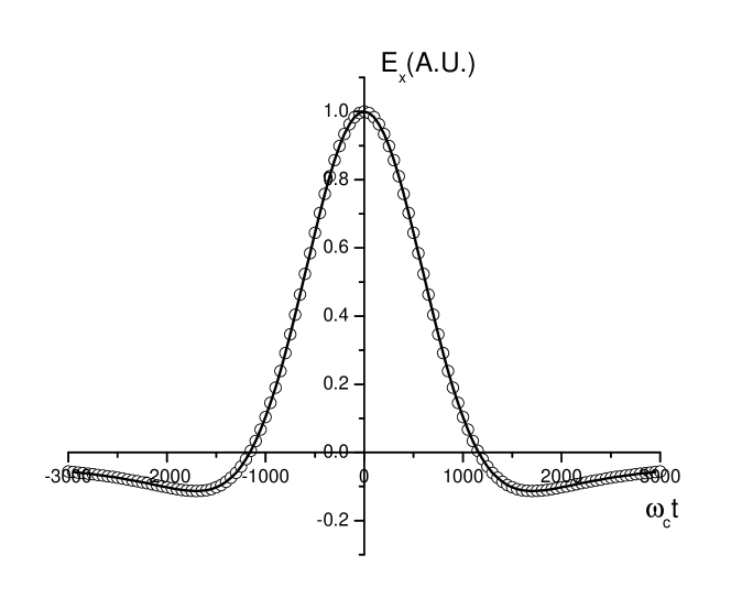
Figure 11: Time structure of a CSR pulse from a Gaussian electron bunch moving in a circle. Here $\theta=0$. Circles present the results obtained from direct superposition of single particle pulses, while the solid line corresponds to the shape calculated by means of (20). The rms bunch length is $\sigma_{\mathrm{T}}=100\lambda_{\mathrm{c}}/c$, where $\lambda_{\mathrm{c}}=4\pi R/(3c\gamma^{3})$

$$F(t)=\frac{1}{\sqrt{2\pi}\sigma_{\mathrm{T}}}\exp\left(-\frac{t^{2}}{2\sigma^{2}_{\mathrm{T}}}\right)\ ,$$

where $\sigma_{\mathrm{T}}$ is the rms electron pulse duration. The rms is assumed to be large, $\sigma_{\mathrm{T}}\gg R/(c\gamma^{3})$. When $\theta=0$ and bunch profile is Gaussian profile, we can write (20) in the form

$$E_{x}(t)=\frac{2(-e)N}{(2\pi)^{1/2}6^{1/3}\sigma^{3}_{\mathrm{T}}\omega^{1/3}_{0}c\mid\vec{r}_{0}\mid}\int\limits^{\infty}_{-\infty}\frac{\varepsilon(t-\tau)\tau}{\mid t-\tau\mid^{1/3}}\exp\left(-\frac{\tau^{2}}{2\sigma^{2}_{\mathrm{T}}}\right)\mathop{\mathrm{d}}\tau\ .$$ (21)

Fig. 11 presents comparative results obtained by means of analytical calculations (solid curve, calculated with (21)) and numerical results (circles, calculated by direct superposition of single pulses from (8)). It is seen from these plots that there is a very good agreement between numerical and analytical results.

It is relevant to make some remarks about the region of applicability of (20). It is important to realize that (20) is valid only when the electrons are moving in a circle and the observer is located in such a way that both the velocity term in Lienard-Wiechert formula can be neglected and the unit vector $\vec{n}$ can be considered constant. Another basic assumption is that the current density changes slowly on the scale of $R/\gamma^{3}$. As a rule, this condition is well satisfied in all practical problems. It should be also mentioned that the above expressions are good approximations only for small enough vertical angles (even though they may be immediately generalized). In fact we used the replacement $\cos\theta\simeq 1$ in the retardation equation and, in practice, such an assumption is valid for the range $\theta^{2}\ll(\sigma/R)^{2/3}$, where $\sigma$ is the characteristic length of electron bunch.

Now we want to extend the latter results to the case of an arc of a circle. At this point we find it convenient to impose the following restriction: we focus only on the radiation seen by an observer lying at large distance from the sources, on the tangent to the electrons orbit at the middle point of the magnet. In this case we can continue to use the fixed coordinate system $(x,y,z)$ shown in Fig. 10. The observation point and the vector $\vec{n}$ are within the $(y,z)$-plane and radiation is emitted at an angle $\theta$ with respect to the $z$-axis. Let us start expressing the total CSR pulse as a superposition of single particle fields at the given position in the far zone. In the case of an arc of a circle equation (8) modifies as follows:

$$\vec{E}_{\mathrm{CSR}}(t)=\int\limits^{t+T}_{t-T}\vec{E}_{\mathrm{r}}(t-\tau)NF(\tau)\mathop{\mathrm{d}}\tau\ .$$ (22)

Here the time $T$ in the integration limits is in loco of a window function in the integrand, in order to cut the contributions of the single particle radiation pulse when the electron is not in the arc. This expression contains the observation time $T$, which should be replaced by the retarded time $t^{\prime}_{\mathrm{e}}$. The two times are related by

$$2T=t^{\prime}_{\mathrm{e}}+\frac{1}{c}\mid\vec{r}(t^{\prime}_{\mathrm{e}})\mid-\frac{1}{c}\mid\vec{r}_{0}\mid\ ,$$

where $t^{\prime}_{\mathrm{e}}=\phi_{\mathrm{m}}/(\omega_{0})$ and $\phi_{\mathrm{m}}$ is the bending magnet angular extension. Our analysis focuses on the case of a long bending magnet, $\gamma\phi_{\mathrm{m}}\gg 1$. Using (6) and (7), the field of the CSR pulse is readily shown to be

$$\vec{E}_{\mathrm{CSR}}(t)=\int\limits^{t-\delta}_{t-T}\vec{E}_{\mathrm{r}}(t-\tau)NF(\tau)\mathop{\mathrm{d}}\tau-NF(t)\int\limits^{t-\delta}_{-\infty}\vec{E}_{\mathrm{r}}(t-\tau)\mathop{\mathrm{d}}\tau$$

$$+\int\limits^{t+T}_{t+\delta}\vec{E}_{\mathrm{r}}(t-\tau)NF(\tau)\mathop{\mathrm{d}}\tau-NF(t)\int\limits^{\infty}_{t+\delta}\vec{E}_{\mathrm{r}}(t-\tau)\mathop{\mathrm{d}}\tau\ .$$ (23)

As we have already done previously, we assume that $\delta$ satisfies condition (10). Adding and subtracting suitable edge terms one can still perform integration by parts, thus obtaining:

$$\vec{E}_{\mathrm{CSR}}(t)=NF(t+T)\int\limits^{t+T}_{-\infty}\vec{E}_{\mathrm{r}}(t-\tau)\mathop{\mathrm{d}}\tau-NF(t-T)\int\limits^{t-T}_{-\infty}\vec{E}_{\mathrm{r}}(t-\tau)\mathop{\mathrm{d}}\tau$$

$$-\int\limits^{t-\delta}_{t-T}\Phi\left[\vec{E}_{\mathrm{r}}\right](t-\tau)N\frac{\mathop{\mathrm{d}}F(\tau)}{\mathop{\mathrm{d}}\tau}\mathop{\mathrm{d}}\tau-\int\limits^{t+T}_{t+\delta}\Phi\left[\vec{E}_{\mathrm{r}}\right](t-\tau)N\frac{\mathop{\mathrm{d}}F(\tau)}{\mathop{\mathrm{d}}\tau}\mathop{\mathrm{d}}\tau\ .$$ (24)

Since condition (10) holds for $\delta$ we may substitute the 3rd and the 4th integral in (24) with a single integral in which the primitive, $\Phi\left[\vec{E}_{\mathrm{r}}\right]$, is substituted by its asymptotic for large values of the argument, $\Phi\left[\vec{E}^{\mathrm{A}}_{\mathrm{r}}\right]$. Under the assumption of a long bending magnet $(\omega_{\mathrm{c}}T\gg 1)$ the 1st and the 2nd integral can be expressed by means of the primitive asymptotic too. Moreover, we can perform a change of variables in all the integrals $t-\tau\to\tau$. As a result expression (24) can be written in the form:

$$\vec{E}_{\mathrm{CSR}}(t)=-NF(t+T)\int\limits^{\infty}_{-T}\vec{E}^{\mathrm{A}}_{\mathrm{r}}(\tau)\mathop{\mathrm{d}}\tau-NF(t-T)\int\limits^{T}_{\infty}\vec{E}^{\mathrm{A}}_{\mathrm{r}}(\tau)\mathop{\mathrm{d}}\tau$$

$$-\int\limits^{T}_{-T}\Phi\left[\vec{E}^{\mathrm{A}}_{\mathrm{r}}\right](\tau)N\frac{\mathop{\mathrm{d}}F(t-\tau)}{\mathop{\mathrm{d}}\tau}\mathop{\mathrm{d}}\tau\ .$$ (25)

Using the ultrarelativistic approximation we can calculate a primitive $\Phi\left[\vec{E}_{\mathrm{r}}\right]$ using (16) and (17). Again we assume that the vertical angle is very small so that we may use the replacement $\cos\theta\simeq 1$. In this situation we have

$$\frac{\vec{n}\times[(\vec{n}\times\vec{\beta})]}{(1-\vec{n}\cdot\vec{\beta})}\simeq\frac{\omega_{0}t^{\prime}\vec{e}_{x}+\theta\vec{e}_{y}}{(\omega_{0}t^{\prime})^{2}/2}$$

This quantity must be evaluated at the retarded time $t^{\prime}\simeq[6\tau/\omega^{2}_{0}]^{1/3}$. Substitution these expressions in (25) gives

$$\vec{E}_{\mathrm{CSR}}(t)=\frac{2eN}{c\mid\vec{r}_{0}\mid}\left\{\int\limits^{T}_{-T}\left[\frac{\varepsilon(\tau)\vec{e}_{x}}{[6\omega_{0}\mid\tau\mid]^{1/3}}+\frac{\theta\vec{e}_{y}}{[6\omega_{0}\mid\tau\mid]^{2/3}}\right]\frac{\mathop{\mathrm{d}}F(t-\tau)}{\mathop{\mathrm{d}}\tau}\mathop{\mathrm{d}}\tau\right.$$

$$\left.+\left[F(t+T)+F(t-T)\right]\frac{\vec{e}_{x}}{(6\omega_{0}T)^{1/3}}\right.$$

$$\left.-\left[F(t+T)-F(t-T)\right]\frac{\theta\vec{e}_{y}}{(6\omega_{0}T)^{2/3}}\right\}\ ,$$ (26)

where $T=\phi_{\mathrm{m}}^{3}/(12\omega_{0})$.

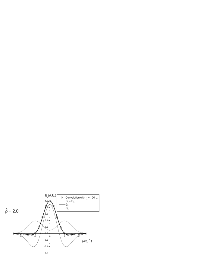
Figure 12: Time structure of the CSR pulse from a Gaussian electron bunch moving along an arc of a circle. Here $\theta=0,\ \hat{\rho}=\phi^{3}_{\mathrm{m}}/(6\omega_{0}\sigma_{\mathrm{T}})=2$. The physical meaning of the magnet length parameter $\hat{\rho}$ will be clear after reading Section 3.3. Circles present the results obtained from direct superposition of single particle pulses. The solid line corresponds to the shape calculated by means of (26)

As an example of the application of this expression, consider the situation when $\theta=0$ and bunch profile is a Gaussian. According to (26) the CSR field in this case is given by

$$E_{x}(t)=G_{1}(t)+G_{2}(t)$$

where

$$G_{1}=\frac{2(-e)N}{(2\pi)^{1/2}6^{1/3}\sigma_{\mathrm{T}}^{3}\omega^{1/3}_{0}c\mid\vec{r}_{0}\mid}\int\limits^{T}_{-T}\frac{\varepsilon(\tau)(t-\tau)}{\mid\tau\mid^{1/3}}\exp\left(-\frac{(t-\tau)^{2}}{2\sigma^{2}_{\mathrm{T}}}\right)\mathop{\mathrm{d}}\tau\ ,$$

$$G_{2}=\frac{2eN}{(2\pi)^{1/2}6^{1/3}\sigma_{\mathrm{T}}(\omega_{0}T)^{1/3}c\mid\vec{r}_{0}\mid}\left[\exp\left(-\frac{(t+T)^{2}}{2\sigma^{2}_{\mathrm{T}}}\right)+\exp\left(-\frac{(t-T)^{2}}{2\sigma^{2}_{\mathrm{T}}}\right)\right]\ .$$

Fig. 12 presents the results of calculations with the analytical formula (26). Comparison with numerical results shows a very good agreement.

3.2 Radiation field in the frequency domain

Let us now go back to our single particle treatment and proceed to the calculation of the spectrum of the electromagnetic radiation produced by an electron during a dipole magnet pass. We know that, in general, for any kind of motion

$$\frac{\mathop{\mathrm{d}}^{2}W}{\mathop{\mathrm{d}}\Omega\mathop{\mathrm{d}}t}=\frac{c\mid\vec{r}\mid^{2}\mid\vec{E}(t)\mid^{2}}{4\pi}\ .$$

Here $\mid\vec{E}\mid^{2}$ is the squared modulus of the electromagnetic field vector at the observation point. The stationary observer who is detecting the radiation emitted into the solid angle $\mathop{\mathrm{d}}\Omega$ measures the total energy as

$$\frac{\mathop{\mathrm{d}}W}{\mathop{\mathrm{d}}\Omega}=\frac{c\mid\vec{r_{0}}\mid^{2}}{4\pi}\int\limits^{\infty}_{-\infty}\mid\vec{E}_{\mathrm{r}}(t)\mid^{2}\mathop{\mathrm{d}}t\ ,$$

where we used the fact that, in the far field approximation, the distance $\mid\vec{r}\mid$ is much larger than $\mid\vec{R}\mid$ , and the zero order expansion reads $\mid\vec{r}(t^{\prime})\mid=\mid\vec{r}_{0}\mid$ (see Fig. 1). From the discussion above, we know that the radiation pulse is emitted over a very short period of time so that the only finite contribution to this integral comes from times close to $t=0$. Extension of the integral to infinite times is only a mathematical convenience which does not affect the physical result.

The general method to derive the frequency spectrum is to transform the electric field from the time domain to the frequency domain.Expressing the electrical field $\vec{E}_{\mathrm{r}}(t)$ by its Fourier transform, we set

$$\vec{E}_{\mathrm{r}}(\omega)=\int\limits^{\infty}_{-\infty}\vec{E}_{\mathrm{r}}(t)\exp(-\mathop{\mathrm{i}}\omega t)\mathop{\mathrm{d}}t\ .$$ (27)

Applying Parseval’s theorem we have

$$\int\limits^{\infty}_{-\infty}\mid\vec{E}_{\mathrm{r}}(\omega)\mid^{2}\mathop{\mathrm{d}}\omega=2\pi\int\limits^{\infty}_{-\infty}\mid\vec{E}_{\mathrm{r}}(t)\mid^{2}\mathop{\mathrm{d}}t$$

and the total absorbed radiation energy from a single pass is therefore

$$\frac{\mathop{\mathrm{d}}W}{\mathop{\mathrm{d}}\Omega}=\frac{c}{8\pi^{2}}\mid\vec{r_{0}}\mid^{2}\int\limits^{\infty}_{-\infty}\mid\vec{E}_{\mathrm{r}}(\omega)\mid^{2}\mathop{\mathrm{d}}\omega\ .$$

Evaluating the electric field by Fourier components we derive an expression for the spectral distribution of the radiation energy

$$\frac{\mathop{\mathrm{d}}^{2}W}{\mathop{\mathrm{d}}\omega\mathop{\mathrm{d}}\Omega}=\frac{c}{4\pi^{2}}\mid\vec{r_{0}}\mid^{2}\mid\vec{E}_{\mathrm{r}}(\omega)\mid^{2}$$ (28)

In order to calculate the Fourier transform we can use (5) and note that the electric field is expressed in terms of quantities at the retarded time $t^{\prime}$. The calculation is simplified if we express the whole integrand in (27) at the retarded $t^{\prime}$ remembering $t^{\prime}=t-\frac{1}{c}\mid\vec{r}(t^{\prime})\mid$:

$$\vec{E}_{\mathrm{r}}(\omega)=\frac{(-e)}{c\mid\vec{r}\mid}\int\limits^{\infty}_{-\infty}\left[\frac{\vec{n}\times[(\vec{n}-\vec{\beta})\times\dot{\vec{\beta}}]}{(1-\vec{n}\cdot\vec{\beta})^{2}}\right]\exp[\mathop{\mathrm{i}}\omega(t^{\prime}+\mid\vec{r}\mid/c)]\mathop{\mathrm{d}}t^{\prime}\ .$$

Since the distance $\mid\vec{r}(t^{\prime})\mid$ is much larger than $\mid\vec{R}\mid$ , the zero order approximation would make $\mid\vec{r}(t^{\prime})\mid=\mid\vec{r}_{0}\mid$ (see Fig. 1). However, such approximation is not good enough in the exponential factor and we must take the next approximation order writing $\mid\vec{r}(t^{\prime})\mid=\mid\vec{r}_{0}\mid-\vec{n}\cdot\vec{R}(t^{\prime})$. Therefore we get

$$\vec{E}_{\mathrm{r}}(\omega)=\frac{(-e)}{c\mid\vec{r}_{0}\mid}\int\limits^{\infty}_{-\infty}\left[\frac{\vec{n}\times[(\vec{n}-\vec{\beta})\times\dot{\vec{\beta}}]}{(1-\vec{n}\cdot\vec{\beta})^{2}}\right]\exp[\mathop{\mathrm{i}}\omega(t^{\prime}-\vec{n}\cdot\vec{R}(t^{\prime})/c)]\mathop{\mathrm{d}}t^{\prime}\ .$$ (29)

We established some basic equations in the frequency domain with which we can start calculations for individual problems. Analytical calculations can be performed without big difficulty in two limiting cases, namely the case of circular motion and ”short” magnet.

3.2.1 Radiation from circular motion

In his paper on synchrotron radiation, Schwinger gives remarkable formulas for the radiation spectrum in the case of an electron moving in a circle [4]. One can find textbooks telling that Schwinger’s formulas apply to the analysis of synchrotron radiation from an electron moving along the arc of a circle too (see for example [8]). This extension is not a physical law: it is merely the statement of an approximation which is valid about the entire wavelength range interesting for the ordinary user. In this context, a critical study of the theoretical status of Schwinger’s formulas seems to be of considerable importance.

We are going to apply (29) to our analysis of synchrotron radiation from circular motion taking advantage of an expression we previously used in Section 3.1: in the case of circular motion $\vec{E}_{\mathrm{r}}(\omega)$ can be evaluated remembering that

$$\frac{\mathop{\mathrm{d}}}{\mathop{\mathrm{d}}t^{\prime}}\left[\frac{\vec{n}\times[(\vec{n}\times\vec{\beta})]}{(1-\vec{n}\cdot\vec{\beta})}\right]=\left[\frac{\vec{n}\times[(\vec{n}-\vec{\beta})\times\dot{\vec{\beta}}]}{(1-\vec{n}\cdot\vec{\beta})^{2}}\right]\ ,$$

Integration by parts yields

$$\int\limits^{\infty}_{-\infty}\left[\frac{\vec{n}\times[(\vec{n}-\vec{\beta})\times\dot{\vec{\beta}}]}{(1-\vec{n}\cdot\vec{\beta})^{2}}\right]\exp[\mathop{\mathrm{i}}\omega(t^{\prime}-\vec{n}\vec{R}(t^{\prime})/c)]\mathop{\mathrm{d}}t^{\prime}$$

$$=\left.\frac{\vec{n}\times[\vec{n}\times\vec{\beta}]}{(1-\vec{n}\cdot\vec{\beta})}\exp\left[\mathop{\mathrm{i}}\omega(t^{\prime}-\vec{n}\cdot\vec{R}(t^{\prime})/c)\right]\right|^{t^{\prime}=\infty}_{t^{\prime}=-\infty}$$

$$-\mathop{\mathrm{i}}\omega\int\limits^{\infty}_{-\infty}\vec{n}\times[\vec{n}\times\vec{\beta}]\exp\left[\mathop{\mathrm{i}}\omega(t^{\prime}-\vec{n}\cdot\vec{R}(t^{\prime})/c)\right]\mathop{\mathrm{d}}t^{\prime}\ .$$ (30)

The reason for using integration by parts is that the contribution from the first term (which to be evaluated at $t^{\prime}=\pm\infty$) is zero. Thus we can write

$$\frac{\mathop{\mathrm{d}}^{2}W}{\mathop{\mathrm{d}}\omega\mathop{\mathrm{d}}\Omega}=\frac{e^{2}\omega^{2}}{4\pi^{2}c}\left|\int\limits^{\infty}_{-\infty}\vec{n}\times[\vec{n}\times\vec{\beta}]\exp\left[\mathop{\mathrm{i}}\omega(t^{\prime}-\vec{n}\cdot\vec{R}(t^{\prime})/c)\right]\mathop{\mathrm{d}}t^{\prime}\right|^{2}\ .$$ (31)

We must emphasize, however, that this expression is not valid in general, but only when a particle is moving in a circle.

The integrand in (31) can be expressed in components to simplify the integration. If we look in the plane of the circle, radiation does not depend upon the azimuthal angle. There is a better way to write out the integrand in (31) by making use of the azimuthal symmetry, which allow one to use again the fixed coordinate system $(x,y,z)$ shown in Fig. 10. The observation point is far away from the source point and we focus on the radiation that is centered about the tangent to the orbit at the source point. The observation point $P$ and the vector $\vec{r}$ and $\vec{n}$ are therefore within the $(y,z)$-plane and radiation is emitted at angle $\theta$ with respect to the $z$-axis. Following the above discussion the azimuthal angle is constant and set to $\phi=\pi/2$. The definition of $\vec{n}$ and $\vec{R}$ can be used to compute the scalar product in the exponential term in (31) so that

$$\vec{n}\cdot\vec{R}=R\cos\theta\sin\omega_{0}t^{\prime}\ ,$$

where $\theta$ is the vertical angle and $\omega_{0}=c/R$. Since the angles are small and the relativistic $\gamma$ factor is large, we can replace

$$\cos\theta\simeq 1-\theta^{2}/2\ ,\quad\sin\omega_{0}t^{\prime}\simeq\omega_{0}t^{\prime}-\omega^{3}_{0}(t^{\prime})^{3}/6\ .$$

Therefore the exponential factor becomes

$$t^{\prime}-\frac{R}{c}\cos\theta\sin\omega_{0}t^{\prime}=\frac{t^{\prime}}{2\gamma^{2}}\left(1+\gamma^{2}\theta^{2}\right)+\frac{c^{2}(t^{\prime})^{3}}{6R^{2}}\ .$$

The triple vector product in (29) can be evaluated in a similar way as

$$\vec{n}\times[\vec{n}\times\vec{\beta}]=\omega_{0}t^{\prime}\vec{e}_{x}+\theta\vec{e}_{y}\ ,$$

We can now write $\vec{E}_{\mathrm{r}}(\omega)$ as

$$\vec{E}_{\mathrm{r}}(\omega)=\frac{(-e)\omega}{c\mid\vec{r}\mid}\left\{\vec{e}_{x}\left[\int\limits^{\infty}_{-\infty}\omega_{0}t^{\prime}\exp\left(\mathop{\mathrm{i}}\omega\left(\frac{t^{\prime}}{2\gamma^{2}}\left(1+\gamma^{2}\theta^{2}\right)+\frac{c^{2}(t^{\prime})^{3}}{6R^{2}}\right)\right)\mathop{\mathrm{d}}t^{\prime}\right]\right.$$

$$\left.+\vec{e}_{y}\left[\int\limits^{\infty}_{-\infty}\theta\exp\left(\mathop{\mathrm{i}}\omega\left(\frac{t^{\prime}}{2\gamma^{2}}\left(1+\gamma^{2}\theta^{2}\right)+\frac{c^{2}(t^{\prime})^{3}}{6R^{2}}\right)\right)\mathop{\mathrm{d}}t^{\prime}\right]\right\}\ .$$ (32)

The integrals in (32) can be expressed in terms of modified Bessel functions as first pointed out by Schwinger [4]. For this we need a change of variables as follows:

$$\tau=\frac{\gamma\omega_{0}t^{\prime}}{(1+\gamma^{2}\theta^{2})^{1/2}}\ ,\quad\xi=\frac{\omega}{2\omega_{\mathrm{c}}}\left(1+\gamma^{2}\theta^{2}\right)^{3/2}\ ,$$

where $\omega_{\mathrm{c}}=3\gamma^{3}\omega_{0}/2$. With these substitutions we get integrals of the form

$$\int\limits^{\infty}_{0}\tau\sin\left(\frac{3}{2}\xi\left(\tau+\frac{1}{3}\tau^{3}\right)\right)\mathop{\mathrm{d}}\tau=\frac{1}{\sqrt{3}}K_{2/3}(\xi)\ ,$$

$$\int\limits^{\infty}_{0}\cos\left(\frac{3}{2}\xi\left(\tau+\frac{1}{3}\tau^{3}\right)\right)\mathop{\mathrm{d}}\tau=\frac{1}{\sqrt{3}}K_{1/3}(\xi)\ ,$$

The Fourier transform of the electrical field (32) finally becomes

$$\vec{E}_{\mathrm{r}}(\omega)=\frac{\sqrt{3}(-e)\omega}{c\mid\vec{r}_{0}\mid\omega_{\mathrm{c}}}\gamma(1+\gamma^{2}\theta^{2})\left[K_{2/3}(\xi)\vec{e}_{x}+\mathop{\mathrm{i}}\frac{\gamma\theta K_{1/3}(\xi)}{(1+\gamma^{2}\theta^{2})^{1/2}}\vec{e}_{y}\right]\ .$$

Using (28) we get an expression for the spectral distribution:

$$\frac{\mathop{\mathrm{d}}^{2}W}{\mathop{\mathrm{d}}\omega\mathop{\mathrm{d}}\Omega}=\frac{3e^{2}\omega^{2}}{4\pi^{2}c\omega^{2}_{\mathrm{c}}}\gamma^{2}(1+\gamma^{2}\theta^{2})^{2}\left[K^{2}_{2/3}(\xi)+\frac{\gamma^{2}\theta^{2}}{1+\gamma^{2}\theta^{2}}K^{2}_{1/3}(\xi)\right]\ .$$ (33)

Quite often an observer is interested in the synchrotron radiation energy emitted over all vertical angles. Integration of equation (33), over the angle $\theta$ gives the required result. We note that the solid angle $\mathop{\mathrm{d}}\Omega=\mathop{\mathrm{d}}\theta\mathop{\mathrm{d}}\phi$ and that radiation does not depend upon the azimuthal angle. So we can write

$$\frac{\mathop{\mathrm{d}}^{2}W}{\mathop{\mathrm{d}}\omega\mathop{\mathrm{d}}\phi}=\frac{3e^{2}\omega^{2}\gamma^{2}}{4\pi^{2}c\omega^{2}_{\mathrm{c}}}\int\limits^{\infty}_{-\infty}(1+\gamma^{2}\theta^{2})^{2}\left[K^{2}_{2/3}(\xi)+\frac{\gamma^{2}\theta^{2}K^{2}_{1/3}(\xi)}{1+\gamma^{2}\theta^{2}}\right]\mathop{\mathrm{d}}\theta\ .$$ (34)

The angle $\theta$ appears in (34) in rather a complicated way which makes it difficult to perform the integration directly. We shall not describe the integration process in detail, not only because it is available in the form of comprehensive treatises [3], but also because this is a pure mathematical problem. If we look it up in [3] we see that (34) can be written as

$$\frac{\mathop{\mathrm{d}}^{2}W}{\mathop{\mathrm{d}}\omega\mathop{\mathrm{d}}\phi}=\frac{\sqrt{3}e^{2}\gamma}{4\pi}\left[\frac{\omega}{\omega_{\mathrm{c}}}\int\limits^{\infty}_{\omega/\omega_{\mathrm{c}}}K_{5/3}(y)\mathop{\mathrm{d}}y\right]\ .$$ (35)

Equation (35) is the required expression for the frequency spectrum of the radiation from an electron moving along a trajectory which is a circle. For a small argument $\omega/\omega_{\mathrm{c}}\ll 1$ we may apply an asymptotic approximation for the modified Bessel’s function and get

$$\frac{\omega}{\omega_{\mathrm{c}}}\int\limits^{\infty}_{\omega/\omega_{\mathrm{c}}}K_{5/3}(y)\mathop{\mathrm{d}}y\simeq 1.33\left(\frac{\omega}{\omega_{\mathrm{c}}}\right)^{1/3}\quad{\mathrm{for}}\quad\omega/\omega_{\mathrm{c}}\ll 1\ .$$

Figure 13: Radiation field from an electron moving along a circle in the time and in the frequency domain

Figure 14: Radiation field from an electron moving along an arc of a circle in the time and in the frequency domain

Figure 15: Radiation field from an electron moving along a short bending magnet in the time and in the frequency domain

Most textbooks on synchrotron radiation discuss equation (35). However, no attention is usually paid to the region of applicability of this equation. Calculations which led to (35) are only valid for an electron moving in a circle. On the other hand we want to study synchrotron radiation from a dipole magnet too. Consider what would happen if, instead of an electron moving in a circle, we had an electron which moves along the arc of a circle. Fig. 13-15 sketch the expected frequency spectrum. These figures provide an illustration of the transition from the usual synchrotron radiation by an electron in a circle to radiation by an electron moving along an arc of a circle. The first sketch (Fig. 13) describes radiation from a circle. It is useful to consider further the relationship between the time domain and the frequency domain. The frequency spectrum of the radiation pulse is given by the expression (35): the Fourier transform at $\omega=0$, $\bar{E}(0)$, is zero because $E(t)$ averages to zero (see Fig. 3).

In the case of dipole magnet, things are quite different. The frequency spectrum may be obtained calculating the Fourier transform of the time distribution of the electric field at the observer’s position. It can be obtained numerically without much work by noticing that we can use curves in Fig. 5-7. As a result, we can define general properties of the spectrum without any analytical calculations. Consider Fig. 14, 15. As these curves illustrate, when the electron moves along an arc of a circle, the spectral distribution does not tend to zero when $\omega\to 0$. Although this fact may look surprising, this is quite natural, since the average of the electric field over time is nonzero when an electron moving along the arc of a circle.

3.2.2 Radiation from an electron moving along the arc of a circle

Many texts on synchrotron radiation theory do not seem to provide a derivation of the expression for the radiation spectrum from an electron moving along an arc of a circle. Here we present such a derivation, which we believe to be quite simple and instructive. Analytical studies of this problem were first performed in [5]. A similar treatment may also be found in the book [9]. Our consideration is restricted to the simplest case from an analytical point of view, namely the case of a bending angle $\phi_{\mathrm{m}}$ very small compared with the $1/\gamma$. No assumptions on the magnetic field parameters have been made to derive the radiation spectrum in the form of equation (29): therefore, our starting point is the same as that for the radiation spectrum calculation from a circular motion in the previous subsection. Introducing the notation

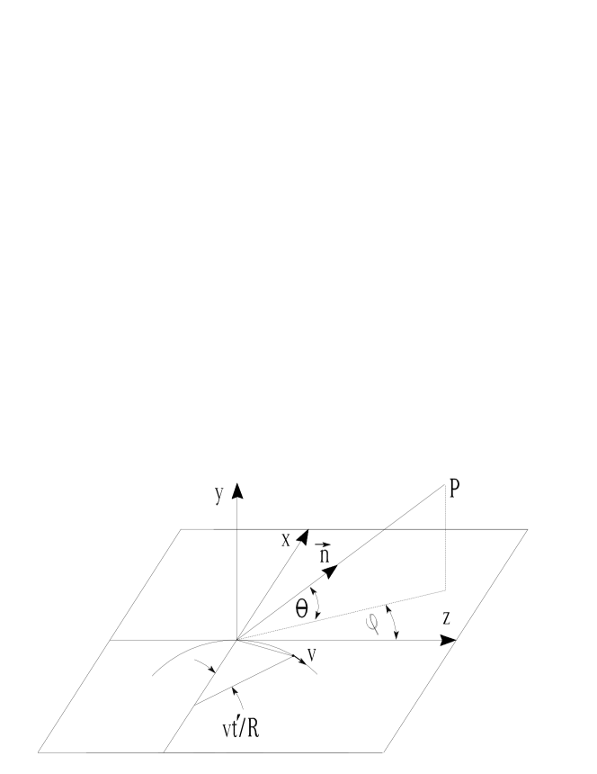
Figure 16: Geometry for synchrotron radiation from an electron moving along an arc of a circle

$$\vec{G}(t^{\prime})=\left[\frac{\vec{n}\times[(\vec{n}-\vec{\beta})\times\dot{\vec{\beta}}]}{(1-\vec{n}\cdot\vec{\beta})^{2}}\right]\ ,$$

we rewrite (29) in the form:

$$\vec{E}_{\mathrm{r}}(\omega)=\frac{(-e)}{c\mid\vec{r}_{0}\mid}\int\limits^{\infty}_{-\infty}\vec{G}(t^{\prime})\exp[\mathop{\mathrm{i}}\omega(t^{\prime}-\vec{n}\cdot\vec{R}(t^{\prime})/c)]\mathop{\mathrm{d}}t^{\prime}\ ,$$

Now we have to perform the integration. The function $\vec{G}(t^{\prime})$ is a smooth curve and does not vary very much across the very narrow bending angle region in the case of a short magnet: therefore we may replace it by a constant. In other words, we simply take $\vec{G}(t^{\prime})$ outside the integral sign and call it $\vec{G}_{0}$. In this case the integral over $t^{\prime}$ in the latter equation is calculated analytically

$$\vec{E}_{\mathrm{r}}(\omega)=\frac{(-e)\vec{G}_{0}}{c\mid\vec{r}_{0}\mid}\int\limits^{L_{\mathrm{m}}/(2c\beta)}_{-L_{\mathrm{m}}/(2c\beta)}\exp[\mathop{\mathrm{i}}\omega(t^{\prime}-\vec{n}\vec{R}(t^{\prime})/c)]\mathop{\mathrm{d}}t^{\prime}$$

$$=\frac{(-e)\vec{G}_{0}L_{\mathrm{m}}}{c\mid\vec{r}_{0}\mid}\frac{\sin\left[(1-\vec{n}\vec{\beta})\omega L_{\mathrm{m}}/(2c\beta)\right]}{\left[(1-\vec{n}\cdot\vec{\beta})\omega L_{\mathrm{m}}/(2c\beta)\right]}\ .$$ (36)

Next we compute the quantities required for expressing explicitly the latter equation. If the system has no azimuthal symmetry, the angular distribution of radiation depends on two variables. These may be taken (Fig. 16) to be the angle $\theta$ between $\vec{n}$ and the $x-z$ plane, and the azimuthal angle $\phi$. We can now write down the components of the vectors $\vec{\beta}$, $\dot{\vec{\beta}}$, and $\vec{n}$ as:

$$\vec{\beta}=\beta\vec{e}_{z}\ ,\quad\dot{\vec{\beta}}=\dot{\beta}\vec{e}_{x}=\frac{\beta^{2}c}{R}\vec{e}_{x}\ ,$$

$$\vec{n}=\cos\theta\sin\phi\vec{e}_{x}+\sin\theta\vec{e}_{y}+\cos\theta\cos\phi\vec{e}_{z}\ .$$

These definitions can be used to get the triple vector product

$$\vec{n}\times[(\vec{n}-\vec{\beta})\times\dot{\vec{\beta}}]=\dot{\beta}\left[\left(\cos^{2}\theta\sin^{2}\phi-1+\beta\cos\theta\cos\phi\right)\vec{e}_{x}\right.$$

$$\left.+\left(\sin\theta\cos\theta\sin\phi\right)\vec{e}_{y}+\left(\cos^{2}\theta\cos\phi\sin\phi-\beta\cos\theta\cos\phi\right)\vec{e}_{z}\right]\ .$$ (37)

We can use these expressions to compute the Fourier transform (36). The spectral distribution is proportional to the square of electric field and if we follow through the algebra we find that

$$\frac{\mathop{\mathrm{d}}^{2}W}{\mathop{\mathrm{d}}\omega\mathop{\mathrm{d}}\Omega}=\frac{e^{2}L^{2}_{\mathrm{m}}}{4\pi^{2}R^{2}c}\frac{(A^{2}_{\sigma}+A^{2}_{\pi})}{\left(1-\beta\cos\theta\cos\phi\right)^{4}}\frac{\sin^{2}\left[(1-\beta\cos\theta\cos\phi)\omega L_{\mathrm{m}}/(2c\beta)\right]}{\left[(1-\beta\cos\theta\cos\phi)\omega L_{\mathrm{m}}/(2c\beta)\right]^{2}}\ ,$$

where the following notation has been introduced: $A_{\sigma}=\sin\phi-\beta\sin\theta$ and $A_{\pi}=\cos\theta\cos\phi$. The quantities $A_{\sigma}$, $A_{\pi}$ are characteristics of the $\sigma-$ and $\pi-$ components of the single-particle linearly polarized radiation.

We emphasize the following features of this result. The radiation is very much collimated in the forward direction, most of the energy being emitted within the cone $\Delta\Omega=\Delta\phi\Delta\theta$ of $\gamma^{-2}$. The radiation maximum is reached at $\theta=0,\ \phi=0$. Spectral properties of the radiation are defined by the function $[\sin^{2}\omega/\omega_{\mathrm{c}}]/[\omega/\omega_{\mathrm{c}}]^{2}$, where the critical frequency is $\omega_{\mathrm{c}}=2c/[(1-\beta\cos\theta\cos\phi)L_{\mathrm{m}}]$. The spectrum from an electron in a ”short” magnet is practically ”white noise” spreading from zero up to the frequencies $\omega\simeq\omega_{\mathrm{c}}$. As one can see, the spectral properties of radiation considered here are significantly different from those of synchrotron radiation from an electron moving in a circle .

3.3 Limitations of standard results

As already pointed out, we can decompose the CSR spectrum, $P(\omega)$, into the product of the square modulus of bunch form-factor $\mid\bar{F}(\omega)\mid^{2}$ with the radiation spectrum from one electron $p(\omega)$. To find $\mid\bar{F}(\omega)\mid^{2}$ from $P(\omega)$, one needs the quantity $p(\omega)$, which is usually very difficult to know with great accuracy within the long wavelength range. Actually, as already discussed, the well-known theory of synchrotron radiation uses approximations which are valid under certain conditions, inappropriate under others. In particular, Schwinger approach relies on several assumptions, which we review once again: first, the observer is located in such a way that the velocity term in the Lienard-Wiechert formula can be completely neglected and that the unit vector $\vec{n}$ can be considered constant throughout the electron evolution. Second, a circular trajectory is postulated. Finally, no aperture limitations is considered at all. These assumptions must be analyzed in order to understand how the CSR pulse is altered in realistic situation. In this subsection we will deal separately with all of them.

Let us imagine that our electron bunch moves along an arc of a circle and that there is no aperture limitation. We can take into account, then, effects as a finite distance between the source and observer, a finite magnet length and the presence of velocity fields by means of (8) where the expression for the electric field is given by the strict Lienard-Wiechert formula. Analytical methods are of limited use in the study of CSR in the near zone, and numerical calculations must be selected. The application of similarity techniques allows one to present numerical results in such a way that they are both general and directly applicable to the calculation of specific device situations. The use of similarity techniques enables one not only to reduce the number of parameters but also to reformulate the problem in terms of variables possessing a clear physical interpretation. Each physical factor influencing the CSR production is matched by its own reduced parameter. For the effect under study this reduced parameter is a measure of the corresponding physical effect. When some effect becomes less important for coherent radiation, it simply falls out of the number of the parameters of the problem.

For our present purposes we would like to concentrate completely on the temporal structure of the CSR pulse. For any CSR pulse there exist some characteristic time, which determines the CSR pulse duration. Its magnitude is of order of the inverse of the frequency spread in the CSR beam. The behavior of the CSR pulse profile as a function of dimensionless parameters provides information on the spectrum distortion. To be specific, we consider the case of an electron beam with a Gaussian axial profile of the current density. When comparing the temporal structure of CSR pulses, it is convenient to use a normalized field amplitude: here, the normalization is performed with respect to the maximal field amplitude. The rms electron pulse duration is assumed to be large $\sigma_{\mathrm{T}}\gg R/(c\gamma^{3})$ and we focus on the radiation pulse seen about the tangent to the orbit at the middle point of magnet. When the vertical angle $\theta=0$ the normalized coherent field amplitude $E_{x}(t)/E_{\mathrm{max}}$ is a function of six dimensional parameters:

$$t\ ,\quad v\ ,\quad R\ ,\quad L_{\mathrm{m}}\ ,\quad\sigma_{\mathrm{T}}\ ,\quad\mid\vec{r}_{0}\mid\ .$$

It is relevant to note that only two dimensions (length and time) are sufficient for a full description of the field profile: after appropriate normalization it is a function of four dimensionless parameters only:

$$E_{x}(t)/E_{\mathrm{max}}=\hat{E}_{x}=D(\hat{t},\hat{\sigma},\hat{\rho},\hat{r}_{0})\ ,$$ (38)

where $\hat{t}=t/\sigma_{\mathrm{T}}$ is the dimensionless time, $\hat{\sigma}=\omega_{0}\sigma_{\mathrm{T}}\gamma^{3}$ is the dimensionless electron pulse duration, $\mid\vec{r}_{0}\mid(c\sigma_{\mathrm{T}})^{-1/3}R^{-2/3}$ is the dimensionless distance between source and observer, $\hat{\rho}=\phi^{3}_{\mathrm{m}}/(6\omega_{0}\sigma_{\mathrm{T}})$ is the magnet length parameter. In the general case the universal function $D$ should be calculated numerically by means of strict Lienard-Wiechert formulas.

The changes of scale performed during the normalization process, mean that we are measuring time, bunch length, distance from the source and magnet length as multiples of ”natural” CSR units. There is a physical reason for being able to write the field profile as in (38): let us explain this fact beginning with a qualitative analysis of the radiation from an electron moving in a circle, in the long wavelength asymptotic. Synchrotron radiation is emitted from a rather small area and we need to determine this area for observers whose detection systems collect information over a long time period $\sigma_{\mathrm{T}}$. The radiation pulse length is equal to the time taken for the electron to travel along any arc $AB$, reduced by the time taken for the radiation to travel directly from the arc extreme $A$ to $B$. Between point $A$ and point $B$ we have a deflection angle $\phi$, so that $\sigma_{\mathrm{T}}\simeq R\phi/(\beta c)-2R\sin(\phi/2)/c$, and $\sin(\phi/2)$ can be approximated by $\sin(\phi/2)\simeq\phi/2-\phi^{3}/48$ for small angles. Then the pulse duration reduces to $\sigma_{\mathrm{T}}\simeq R\phi^{3}/(24c)$. The radiation source extends over some finite length $R\phi\simeq L_{\mathrm{f}}=(c\sigma_{\mathrm{T}})^{1/3}R^{2/3}$ along the particle path. We see that the reduced distance can be expressed as $\hat{r}_{0}=\mid\vec{r}_{0}\mid/L_{\mathrm{f}}$. One can find that the ratio $(R\phi_{\mathrm{m}})^{3}/(6L_{\mathrm{f}}^{3})$ is equal to $\hat{\rho}$, which we use now as a measure of finite magnet length effects.

3.3.1 Finite distance effects

Let us imagine that our electron bunch moves in a real circle and there is no aperture limitation. We can first consider the contribution given by the acceleration field alone and then focus on the contributions by the velocity field. When the electron bunch radiates from a circle the spectrum is obviously independent of the $\hat{\rho}$ parameter. In the long wavelength asymptotic $(\hat{\sigma}\gg 1)$ the acceleration field is described by one dimensionless parameter only: $\hat{r}_{0}$, where $\hat{r}_{0}=\mid\vec{r}_{0}\mid(c\sigma_{\mathrm{T}})^{-1/3}R^{-2/3}$ is the dimensionless distance between radiation source and observer.

The region of applicability of Schwinger’s formulas requires the dimensionless distance to have a large value $\hat{r}_{0}\gg 1$. In fact, as previously explained, the radiation source extends over some finite length $R\phi\simeq L_{\mathrm{f}}$, and this length corresponds to a transverse size of the radiation source $d\simeq R\phi^{2}$. The vector $\vec{n}$ changes its orientation between point $A$ and point $B$ of an angle of order $d/r_{0}$, where $r_{0}$ is the distance between source and observer. Our estimates show that in the case $d/r_{0}\ll\phi$, the vector $\vec{n}$ in Lienard-Wiechert formula is almost constant when the electron moves along the formation length $R\phi$. Thus, we can conclude that the unit vector $\vec{n}$ can be considered constant throughout the electron evolution only if $r_{0}\gg L_{\mathrm{f}}$.

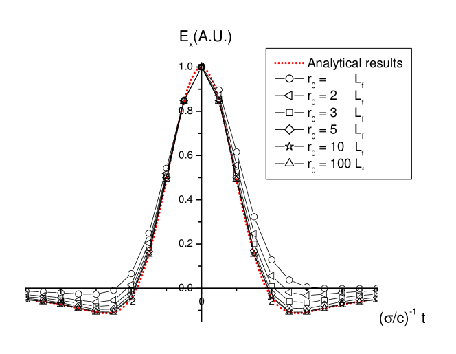
Figure 17: Time structure of a CSR pulse from a Gaussian electron bunch moving in a circle at different reduced distance between source and observer. Here $\theta=0$. The dashed curve is calculated within the far zone approximation (21). Numerical calculations have been performed with strict Lienard-Wiechert formula

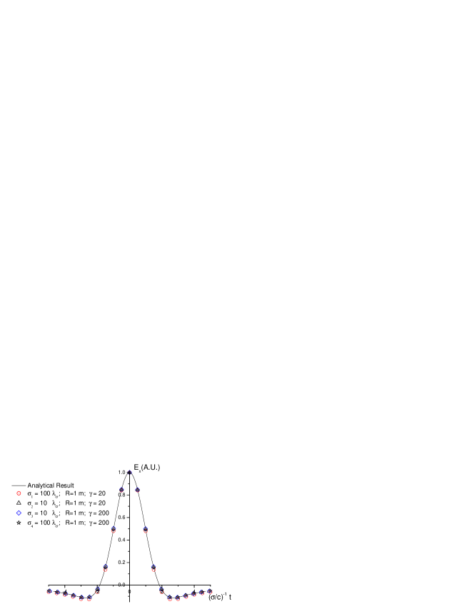
Figure 18: Illustration of similarity techniques. Time structure of a CSR pulse from a Gaussian electron bunch moving in a circle for various sets of parameters. The reduced distance is held constant, $\hat{r}_{0}=15$. The solid curve is calculated within the far zone approximation (21). Numerical calculations have been performed with strict Lienard-Wiechert formula

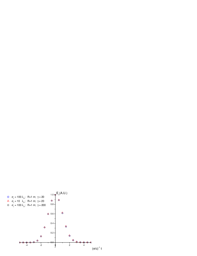
Figure 19: Illustration of similarity techniques. Time structure of a CSR pulse from a Gaussian electron bunch moving in a circle for various sets of parameters. The reduced distance is held constant, $\hat{r}_{0}=0.15$. Numerical calculations have been performed with strict Lienard-Wiechert formula

The results of numerical calculations for several values of $\hat{r}_{0}$ are presented in Fig. 17. Calculations have been performed using the strict Lienard-Wiechert formula. The plots in Fig. 17 give an idea of the region of validity of the far zone approximation considered above. At large distance the CSR pulse profile is simply the far zone profile (21). One can see that (21) works well at $\hat{r}_{0}=100$. Then, at $\hat{r}_{0}=3$, the CSR pulse envelope is visibly modified. As the distance is decreased, the difference between the approximate and the strict pulse profile becomes significant. From a practical point of view this set of plots covers all the region of interest for the distance between observer and sources.

To check that no mistakes have been made in our similarity techniques we evaluate the normalized CSR pulse profile for several sets of problem parameters. The reduced distance is held constant. In the present example, these values are $\hat{r}_{0}=0.15,15$. The plots are calculated, numerically, using the strict Lienard-Wiechert formula. Fig. 18, Fig. 19 show such plots. It is seen that there is a good agreement with the prediction that the acceleration field from a circle in long wavelength asymptotic is a function of the reduced distance only.

3.3.2 Velocity field effects

Usual theory of synchrotron radiation is based on the assumption that acceleration field dominates and all the results presented above refer to the case when there is no influence of the velocity field on the detector. The acceleration field dominates in the far zone only, and we want to study near zone effects too. The physics of coherent effects studied by means of general expressions for the Lienard-Wiechert fields is much richer than that of the simplified radiation field model considered above. In the long wavelength asymptotic the velocity part of the coherent electric field from a particle in a circle is a function of two dimensionless parameters: the reduced distance parameter $\hat{r}_{0}$ and the reduced electron pulse duration parameter $\hat{\sigma}$:

$$E_{\mathrm{(v)}}(t)/E_{\mathrm{max}}=\hat{E}_{\mathrm{(v)}}=D(\hat{t},\hat{\sigma},\hat{r}_{0})\ ,$$ (39)

where the normalization of the velocity field is performed with respect to the maximal acceleration field amplitude.

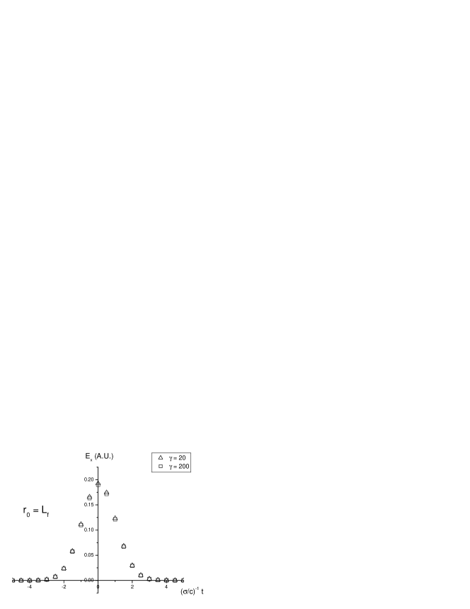
Figure 20: Illustration of similarity techniques. Electric field pulse due to velocity term from a Gaussian electron bunch moving in a circle for various sets of parameters. The reduced distance and reduced bunch length are held constant, $\hat{r}_{0}=1$ and $\hat{\sigma}_{\mathrm{T}}=100$ respectively. Numerical calculations have been performed with strict Lienard-Wiechert formula

To show that this is correct we can perform a simple check. In Fig. 20 we present numerical calculation results for the velocity field for different sets of parameters. The reduced distance and the reduced electron pulse duration are held constant. It is seen that all numerical results agree rather well. Therefore the plots in Fig. 20 convince us that the dimensionless equation (39) provides an adequate description of the numerical calculations.

Fig. 21 and Fig. 22 show the dependence of the normalized velocity field amplitude on the value of the reduced electron pulse duration for different values of the reduced distance. Using these plots we can give a quantitative description of the region of applicability of the radiation field model. It is seen from the plots in Fig. 22 that in the near zone we cannot neglect the influence of the velocity field on the detector.

Let us now estimate the importance of the velocity field effect. Let us start considering the total velocity field pulse as a superposition of single particle fields at a given position in the far zone. To calculate the integral one should take into account the property of its kernel. In the far zone the velocity field from one electron is close to an antisymmetric function and the average of the electric field over time is close to zero. The approach used in section 3.1 can be also used to compute the coherent velocity field. Under the long electron bunch condition the kernel (velocity field from one electron) can be substituted by its asymptotic behavior. If we wish to estimate the normalized amplitude of the coherent velocity field we can get it simply by dividing the asymptotic behavior of the velocity field kernel by the asymptotic behavior of the acceleration field kernel, so that, in the far zone, the normalized velocity field is of order $E_{\mathrm{v}}/E_{\mathrm{acc}}\simeq R/(\gamma^{2}\theta^{2}r_{0})$, where $\theta\simeq(c\sigma_{\mathrm{T}}/R)^{1/3}$ is the natural synchrotron radiation opening angle with frequency $\omega\simeq\sigma^{-1}_{\mathrm{T}}\ll c\gamma^{3}/R$. Using normalized variables we get

$$\hat{E}_{\mathrm{(v)}}\simeq\hat{r}^{-1}_{0}\hat{\sigma}^{-2/3}\quad{\mathrm{for}}\quad\hat{\sigma},\ \hat{r}_{0}\gg 1\ .$$

As we can see from Fig. 21, numerical calculations in the far zone confirm this simple physical consideration. The value of $\hat{E}_{\mathrm{v}}$ that we can expect is found remembering that, in the example given in Fig. 21, $\hat{r}_{0}=100,\ \hat{\sigma}=100$; therefore the normalized velocity field would be about 0.0004, which is the same order of magnitude as results of numerical calculations (0.0002). Also, $\hat{E}_{\mathrm{v}}$ varies roughly as $\hat{\sigma}^{-2/3}$.

The normalized velocity field amplitude decreases, as we see from our estimations, linearly with distance, which means that if we are in the near zone at $\hat{r}_{0}=1$ there will be $\hat{E}_{\mathrm{v}}\simeq 0.04$. Numerical calculation results show that, at the value $\hat{r}_{0}=1$, we have $\hat{E}_{\mathrm{v}}=0.2$. We should say that our approximate treatment of coherent velocity field breaks down once source and observer get as close as they are at $\hat{r}_{0}\simeq 1$. We have, however, a simple explanation for that. In addition to the antisymmetric part of kernel we have just described, there is also a symmetric part. When source and observer are far apart the observer sees only the antisymmetric part and the average of electric field from one electron is close to zero. At very close distances there begins to be some extra symmetric part of the kernel. This symmetric field, which also varies with the separation, should be, of course, included in more precise estimates.

Figure 21: Electric field pulse due to velocity term from a Gaussian electron bunch moving in a circle at different reduced bunch length. The reduced distance is held constant, $\hat{r}_{0}=100$. Here $\theta=0$ and the normalization is performed with respect to the maximal acceleration field amplitude

Figure 22: Electric field pulse due to velocity term from a Gaussian electron bunch moving in a circle at different reduced bunch length. The reduced distance is held constant, $\hat{r}_{0}=1$. Here $\theta=0$ and the normalization is performed with respect to the maximal acceleration field amplitude

3.3.3 Finite magnet length effects

Until now we have considered the case in which electrons moves in a circle. Here we will generalize this situation and study the case where the electrons move along an arc of a circle. In order to fully characterize the magnet length required to assure the accuracy of the circular motion model, it is necessary to specify the distortion of Schwinger spectrum associated with all interesting magnet lengths in an experiment. Normalizing equation (26), we obtain that, under the far field approximation, the CSR pulse profile is a function of only one dimensionless parameter $\hat{\rho}=\phi_{\mathrm{m}}^{3}/(6\omega_{0}\sigma_{\mathrm{T}})$, where $\phi_{\mathrm{m}}$ is the magnet angular extension. The region of applicability of Schwinger’s formulas require the parameter $\hat{\rho}$ to have a large value $\hat{\rho}\gg 1$. Using the plots presented in Fig. 23, one can characterize quantitatively the region of applicability of the circular motion model.

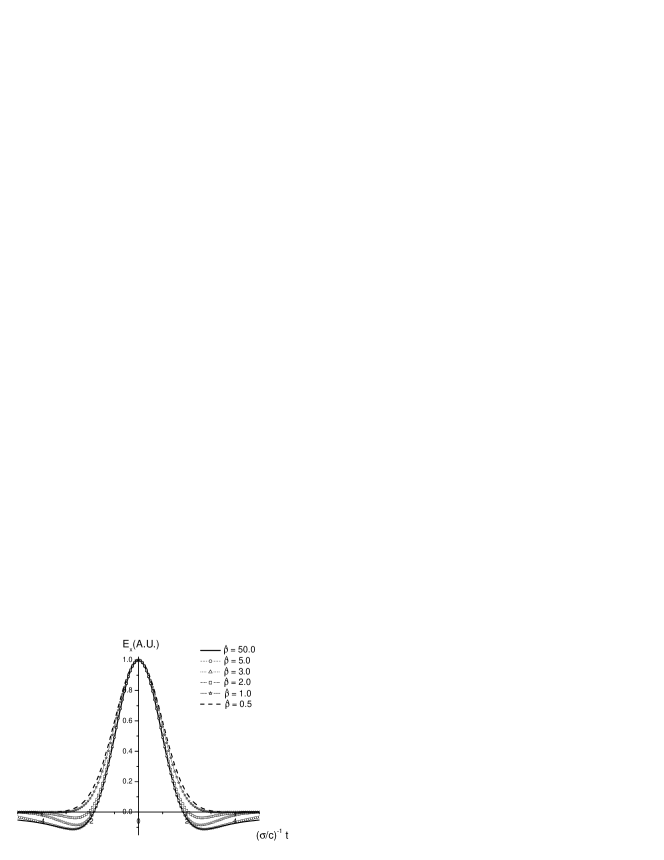
Figure 23: Time structure of a CSR pulse in the far zone from a Gaussian electron bunch moving along an arc of a circle at different reduced magnet lengths. Here $\theta=0$. Calculations have been performed with anaytical formula (26). Results at $\hat{\rho}=50$ (solid curve) agree with our analytical expression (21) for circular motion within 1%

3.3.4 Diffraction effects

Another problem concerns radiation spectrum distortions: this has to do with aperture limitations. In real accelerators, the long wavelength synchrotron radiation from bending magnets integrates over many different vacuum chamber pieces with widely varying aperture. The SR spectrum formed by such a system will be perturbed by the presence of an aperture and we should seek a mathematical mean for predicting these perturbations.

One may wonder how the existence of an aperture in an accelerator vacuum chamber and in a beam line, which is relatively far from the source, can influence the synchrotron radiation spectrum. To illustrate this point, we consider the situation shown in Fig. 24. The object of interest is an electron moving in a circle. Between the observer and the source there is an aperture with a characteristic dimension $d$. Qualitatively, an observer looking at a single electron is presented with a cone of radiation characterized by an aperture angle of order $\theta\simeq\sqrt{d/R}$. Fig. 24 shows part of the trajectory of an electron travelling along an arc of a circle of radius $R$. At first glance this intuitive argument indicates that the frequency spectrum may be obtained by reducing the situation shown in Fig. 24 to Fig. 4 and simply calculating radiation from an electron moving along a trajectory which is an arc of a circle. However, the situation is more complicated than that. The field at $P$ can be represented as a sum of two parts - the field due to the source plus the field due to the wall, i.e. due to the motions of the charges in the wall. The latter kind of radiation field can be described in terms of diffraction theory. Diffraction is the process by which radiation is redirected near sharp edges. As it propagates away from these sharp edges, it interferes with nearby non-diffracted radiation, producing interference patterns. A finite aperture introduces, therefore, diffraction effects specific to the geometry and clearly dependent on the wavelength. For structures such as pinholes it is found that these diffraction patterns propagate away from the structure at angles of order $\theta_{\mathrm{d}}\simeq c/\omega d$, where $d$ is the characteristic aperture dimension. The region of applicability for the far diffraction zone where effects play a significant role is given by the relation $L_{\mathrm{a}}\gg L_{\mathrm{d}}\simeq\omega d^{2}/c$, where $L_{\mathrm{a}}$ is the distance between observer and aperture. When the wavelength is about $R\theta^{3}\simeq(d^{3}/R)^{1/2}$, the latter condition transforms to $L_{\mathrm{a}}\gg L_{\mathrm{d}}\simeq R\theta$. This simple physical argument indicates that the situation shown in Fig. 24 at $L_{\mathrm{a}}>R\theta\simeq(Rd)^{1/2}$ cannot be reduced to the situation shown in Fig. 4. The significance of the discussed limitation cannot be fully appreciated until we determine typical values of the parameters that can be expected in practice. For example, if $R=3{\mathrm{m}}$ and $\lambda=100\mu{\mathrm{m}}$, $\theta\simeq 0.03$, so that at distance greater than 10 cm from the aperture, a 1 cm diameter hole would be sufficiently narrow to perturb significantly the synchrotron radiation spectrum at that wavelength.

Figure 24: Depiction of the effects of an aperture limitation. CSR from a circle allows us to measure the bunch profile form-factor in a frequency range down to $\omega_{\mathrm{a}}$ only

The computation of spectrum distortions for practical accelerator applications is a rather difficult problem. One encounters vacuum chamber components which require special attention and sophisticated techniques should be developed to deal with this situation. The character of spectrum distortions largely depends on the actual geometry and on the material of the vacuum chamber, so that we may expect significant complications in the determination of these distortions along a vacuum enclosure of the actual device. The vacuum chamber of an accelerator presents a too complicated geometry to allow an analytical expression for spectrum distortions. In principle each section of the vacuum chamber must be treated individually. By employing two or three-dimensional numerical codes it may be possible to determine the spectrum for a particular component. Yet, every accelerator is somewhat different from another and will have its own particular spectrum distortions. For this reason, in this discussions we focused only on basic ideas about aperture limitations.

4 Radiation from an undulator

To optimally meet the needs for beam diagnostic measurements with the features of synchrotron radiation, it is desirable to provide specific radiation characteristics that cannot be obtained from bending magnets but require special magnetic systems. To generate specific synchrotron radiation characteristics, radiation is often produced by special insertion devices installed along the particle beam path. An insertion device does not introduce a net deflection of the beam and we may therefore choose any arbitrary field strength which is technically feasible to adjust the radiation spectrum to experimental needs. In this Section we discuss the basic theory of one such devices, a planar undulator, and its applications to CSR diagnostics.

4.1 Basic theory of undulator radiation

The magnetic field on the axis of a planar undulator is given by

$$\vec{H}(z)=\vec{e}_{y}H_{\mathrm{w}}\sin(k_{\mathrm{w}}z)\ ,$$

where $\vec{e}_{y}$ is the unit vector directed along the $y$ axis of the Cartesian coordinate system $(x,y,z)$ in Fig. 25. The Lorentz force is used to derive the equation of motion of an electron with energy $\gamma m_{\mathrm{e}}c^{2}$ in the presence of a magnetic field. Integration of this equation gives

$$\vec{v}_{x}(z)=\vec{e}_{x}c\theta_{\mathrm{w}}\cos(k_{\mathrm{w}}z)\ ,$$

where $\theta_{\mathrm{w}}=K/\gamma$ and $K=eH_{\mathrm{w}}/(m_{\mathrm{e}}c^{2}k_{\mathrm{w}})$ is the undulator parameter. It is useful to present another form of this expression convenient for numerical calculations: $K=0.093\times H_{\mathrm{w}}({\mathrm{kGs}})\times\lambda_{\mathrm{w}}({\mathrm{cm}})$ where $\lambda_{\mathrm{w}}=2\pi/k_{\mathrm{w}}$. The transverse and longitudinal velocity components are related by $(\dot{z})^{2}=\beta^{2}c^{2}-(\dot{x})^{2}$, which gives

$$\beta_{z}=\beta_{\mathrm{av}}-\frac{K^{2}}{4\gamma^{2}}\cos 2k_{\mathrm{w}}z\ ,$$

where $\beta_{\mathrm{av}}=\beta[1-K^{2}/(4\gamma^{2})]$ is the mean velocity of the electron along the undulator.

Figure 25: Radiation geometry for the undulator field

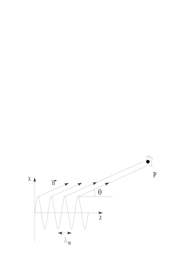
Figure 26: Synchrotron radiation production from successive poles

It is generally assumed that the distance between the undulator and the observation point is much larger than the undulator length. This assumption is usually referred to as far field approximation. Suppose this condition is met. Denoting with $\vec{r}$, as usual, the vector from the electron position at the retarded time to the observation point and with $\vec{r}_{0}$ the vector from the coordinate origin, placed somewhere inside the undulator, to the observation point we compute $\vec{r}\simeq\vec{r}_{0}-\vec{n}\cdot\vec{R}$ with $\vec{n}=\vec{r}_{0}/\mid\vec{r}_{0}\mid$. The unit vector from the retarded source particle to the observer is, from Fig. 25

$$\vec{n}=\cos\phi\sin\theta\vec{e}_{x}+\sin\phi\sin\theta\vec{e}_{y}+\cos\theta\vec{e}_{z}\ .$$

The vector $\vec{R}$, which describes the motion of the electron in the $x-z$ plane, can be obtained from the previous treatment:

$$x(t)=\frac{K}{k_{\mathrm{w}}\gamma}\sin(k_{\mathrm{w}}\beta_{\mathrm{av}}ct)\ ,\quad z(t)=\beta_{\mathrm{av}}ct-\frac{K^{2}}{8k_{\mathrm{w}}\gamma^{2}}\sin(2k_{\mathrm{w}}\beta_{\mathrm{av}}ct)\ .$$

Let us find the Fourier harmonics of the radiation field from an electron moving along the undulator. As in section 3.2, our starting point is equation (29) since, once again, this is a rigorous equation under the assumption of a large distance between observer and radiating electron. Note that the integration in (29) is to be performed over all time but in practice, without loss of generality, it can be restricted to the time during which the electron is passing through the undulator. We can write:

$$\vec{E}_{\mathrm{r}}(\omega)=\frac{(-e)}{c\mid\vec{r}_{0}\mid}\int\limits^{N_{\mathrm{w}}T}_{0}\left[\frac{\vec{n}\times[(\vec{n}-\vec{\beta})\times\dot{\vec{\beta}}]}{(1-\vec{n}\cdot\vec{\beta})^{2}}\right]\exp[\mathop{\mathrm{i}}\omega(t^{\prime}-\vec{n}\cdot\vec{R}(t^{\prime})/c)]\mathop{\mathrm{d}}t^{\prime}\ ,$$ (40)

where $T=\lambda_{\mathrm{w}}/(c\beta_{\mathrm{av}})$, and $N_{\mathrm{w}}$ is the number of undulator periods. The integral in the latter expression can be represented as a sum of $N_{\mathrm{w}}$ integrals over each undulator period (see Fig. 26). Integrating by parts (40) and taking into account the sum of the geometric progression

$$\sum^{N_{\mathrm{w}}}_{n=1}\exp(\mathop{\mathrm{i}}n\phi)=\frac{\sin N_{\mathrm{w}}\phi/2}{\sin\phi/2}\exp\mathop{\mathrm{i}}(N_{\mathrm{w}}+1)\phi/2$$

we find

$$\vec{E}_{\mathrm{r}}(\omega)=\frac{(-e)}{c\mid\vec{r}_{0}\mid}\left\{\left.\frac{\vec{n}\times[\vec{n}\times\vec{\beta}]}{(1-\vec{n}\cdot\vec{\beta})}\exp\left[\mathop{\mathrm{i}}\omega(t^{\prime}-\vec{n}\cdot\vec{R}(t^{\prime})/c)\right]\right|^{t^{\prime}=N_{\mathrm{w}}T}_{t^{\prime}=0}\right.$$

$$\left.-\mathop{\mathrm{i}}\omega\frac{\sin N_{\mathrm{w}}\omega(1-\beta_{\mathrm{av}}n_{z}))T/2}{\sin\omega(1-\beta_{\mathrm{av}}n_{z})T/2}\exp\left[\mathop{\mathrm{i}}(N_{\mathrm{w}}-1)\omega(1-\beta_{\mathrm{av}}n_{z})T/2\right]\right.$$

$$\left.\times\int\limits^{T}_{0}\vec{n}\times[\vec{n}\times\vec{\beta}]\exp\left[\mathop{\mathrm{i}}\omega(t^{\prime}-\vec{n}\cdot\vec{R}(t^{\prime})/c)\right]\mathop{\mathrm{d}}t^{\prime}\right\}\ .$$ (41)

For our purposes, it is most convenient to express the latter equation in the form

$$\vec{E}_{\mathrm{r}}(\omega)=\frac{2\mathop{\mathrm{i}}(-e)}{c\mid\vec{r}_{0}\mid(1-\beta_{\mathrm{av}}\cos\theta)}\exp\left[\mathop{\mathrm{i}}(N_{\mathrm{w}}-1)\omega(1-\beta_{\mathrm{av}}\cos\theta)T/2\right]$$

$$\times\left\{\vec{n}\times[\vec{n}\times\vec{\beta}_{0}]\frac{(1-\beta_{\mathrm{av}}\cos\theta)}{(1-\vec{n}\cdot\vec{\beta}_{0})}\right.$$

$$\left.\times\exp\left[\mathop{\mathrm{i}}\omega(1-\beta_{\mathrm{av}}\cos\theta)T/2\right]\sin\left[N_{\mathrm{w}}\omega(1-\beta_{\mathrm{av}}\cos\theta)T/2\right]\right.$$

$$\left.-\left[\omega(1-\beta_{\mathrm{av}}\cos\theta)T/2\right]\frac{\sin N_{\mathrm{w}}\omega(1-\beta_{\mathrm{av}}\cos\theta)T/2}{\sin\omega(1-\beta_{\mathrm{av}}\cos\theta)T/2}\right.$$

$$\left.\times\frac{1}{T}\int\limits^{T}_{0}\vec{n}\times[\vec{n}\times\vec{\beta}]\exp\left[\mathop{\mathrm{i}}\omega(t^{\prime}-\vec{n}\cdot\vec{R}(t^{\prime})/c)\right]\mathop{\mathrm{d}}t^{\prime}\right\}\ .$$ (42)

Here $c\vec{\beta}_{0}=c\vec{\beta}(0)=c\vec{\beta}(N_{\mathrm{w}}T)$ is the initial and final velocity of the electron. From the shape of the interference function $\sin^{2}(N_{\mathrm{w}}x)/\sin^{2}(x)$ we predict that important contributions to the second term will occur when $x=\omega(1-\beta_{\mathrm{av}}\cos\theta)T/2$ does not differ significantly from the resonance value $x=\pi$. The maximum of the absolute value at resonance is, then, proportional to the number of periods $N_{\mathrm{w}}$ and, on the assumption of $N_{\mathrm{w}}\gg 1$, we can neglect the first term.

The spectral distribution of the radiation energy is given by equation (28). Taking the square modulus of (42) and keeping the resonance term only, we find

$$\frac{\mathop{\mathrm{d}}^{2}W}{\mathop{\mathrm{d}}\omega\mathop{\mathrm{d}}\Omega}=\frac{e^{2}\omega^{2}}{4\pi^{2}c}\left[\frac{\sin N_{\mathrm{w}}\omega(1-\beta_{\mathrm{av}}\cos\theta)T/2}{\sin\omega(1-\beta_{\mathrm{av}}\cos\theta)T/2}\right]^{2}$$

$$\times\left|\int\limits^{T}_{0}\vec{n}\times[\vec{n}\times\vec{\beta}]\exp\left[\mathop{\mathrm{i}}\omega(t^{\prime}-\vec{n}\cdot\vec{R}(t^{\prime})/c)\right]\mathop{\mathrm{d}}t^{\prime}\right|^{2}\ .$$ (43)

Let us now analyze the interference function in (43)

$$f(\omega)=\left[\frac{\sin N_{\mathrm{w}}\omega(1-\beta_{\mathrm{av}}\cos\theta)T/2}{\sin\omega(1-\beta_{\mathrm{av}}\cos\theta)T/2}\right]^{2}$$

and study some of its consequences. The whole curve is localized near

$$\omega=\omega_{\mathrm{res}}=2ck_{\mathrm{w}}\gamma^{2}\left[1+\frac{K_{\mathrm{w}}^{2}}{2}+\gamma^{2}\theta^{2}\right]^{-1}\ .$$

The latter condition is called resonance condition and tells us the radiation frequency as a function of the undulator period $\lambda_{\mathrm{w}}$, the undulator parameter $K_{\mathrm{w}}$, the electron energy $\gamma m_{\mathrm{e}}c^{2}$, and the polar angle of observation $\theta$. Let us concentrate on the radiation produced in the forward direction. In this case $\theta=0$ and there is no vertically polarized radiation. By means of an angular filter, whose principle is shown in Fig. 27, we can obtain the undulator radiation from the central cone. Note that for the radiation within the cone of half angle

$$\theta_{\mathrm{cen}}=\frac{\sqrt{1+K^{2}_{\mathrm{w}}/2}}{\gamma\sqrt{N_{\mathrm{w}}}}\ ,$$

the relative spectral FWHM bandwidth is $\Delta\omega/\omega=0.89/N_{\mathrm{w}}$. This means that we have a very sharp central maximum with very weak subsidiary maxima on the sides. In fact, it is possible to prove that the intensity at the next maximum is less than 5% of the first maximum intensity (see Fig. 28). There is another important feature of the interference function: if the frequency is increased by any multiple of $\omega_{\mathrm{res}}$, we get other strong maxima of interference function at $\omega=2\omega_{\mathrm{res}},\ 3\omega_{\mathrm{res}},\ 4\omega_{\mathrm{res}}$, and so forth. Near each of these maxima the pattern of Fig. 28 is repeated.

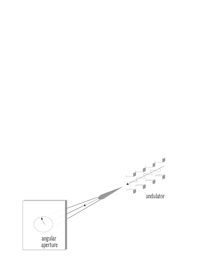
Figure 27: Undulator radiation with an angular filter

Figure 28: Radiated wavetrain from a single electron traversing an undulator, as detected into the central cone, and corresponding spectral distribution function

There is no forward radiation for even harmonics of the fundamental frequency $\omega_{\mathrm{res}}$. Let us briefly justify the latter statement. First let us calculate the integral in (43). At $\theta=0$ the triple vector product is

$$\vec{n}\times[\vec{n}\times\vec{\beta}]=\vec{\beta}-\vec{n}(\vec{n}\cdot\vec{\beta})=\beta_{x}\vec{e}_{x}=\frac{K}{\gamma}\cos(k_{\mathrm{w}}z)\vec{e}_{x}\ .$$ (44)

The exponential factor in (43) can be evaluated in a similar way

$$\exp\left[\mathop{\mathrm{i}}m\omega_{0}(t^{\prime}-\vec{n}\cdot\vec{R}(t^{\prime})/c)\right]=\exp\left[\mathop{\mathrm{i}}mk_{\mathrm{w}}z+\mathop{\mathrm{i}}Q\sin 2k_{\mathrm{w}}z\right]\ ,$$ (45)

where $m$ is integer,

$$Q=K^{2}m\omega_{0}/(8k_{\mathrm{w}}\gamma^{2})=mK^{2}_{\mathrm{w}}/(4+2K^{2}_{\mathrm{w}})\ ,$$

and $\omega_{0}=2\gamma^{2}k_{\mathrm{w}}/[c(1+K^{2}_{\mathrm{w}}/2)]$ is the resonance frequency of the fundamental harmonic at $\theta=0$. Using (44) and (45), together with the expansion

$$\exp[\mathop{\mathrm{i}}Q\sin(2k_{\mathrm{w}}z)]=\sum^{n=+\infty}_{n=-\infty}J_{n}(Q)\exp(2\mathop{\mathrm{i}}nk_{\mathrm{w}}z)\ ,$$

where $J_{n}$ is the Bessel function of order $n$, we obtain:

$$\left|\int\limits^{T}_{0}\vec{n}\times[\vec{n}\times\vec{\beta}]\exp\left[\mathop{\mathrm{i}}m\omega_{0}(t^{\prime}-\vec{n}\cdot\vec{R}(t^{\prime})/c)\right]\mathop{\mathrm{d}}t^{\prime}\right|^{2}=$$

$$\frac{K^{2}}{\gamma^{2}}\left|\sum^{n=+\infty}_{n=-\infty}J_{n}(Q)\int\limits^{\lambda_{\mathrm{w}}}_{0}\cos(k_{\mathrm{w}}z)\exp[\mathop{\mathrm{i}}(2n+m)k_{\mathrm{w}}z]\mathop{\mathrm{d}}z\right|^{2}\ ,$$ (46)

which is non-zero only when $m+2n\pm 1=0$. When $m$ is odd the spectral and angular density of the radiation energy emitted at zero angle by a single electron during the undulator pass is given by the expression

$$\left.\frac{\mathop{\mathrm{d}}^{2}W(\omega_{m})}{\mathop{\mathrm{d}}\omega\mathop{\mathrm{d}}\Omega}\right|_{\theta=0}=\frac{e^{2}N^{2}_{\mathrm{w}}\gamma^{2}m^{2}A_{\mathrm{JJ}}^{2}K^{2}_{\mathrm{w}}}{c(1+K^{2}_{\mathrm{w}}/2)^{2}}\frac{\sin^{2}[\pi N_{\mathrm{w}}(\omega-\omega_{m})/\omega_{m}]}{[\pi N_{\mathrm{w}}(\omega-\omega_{m})/\omega_{m}]^{2}}\ ,$$

where the following notation has been introduced: $\omega_{m}=m\omega_{0}$,

$$A_{\mathrm{JJ}}=[J_{(m-1)/2}(Q)-J_{(m+1)/2}(Q)]\ .$$

When deriving the latter expression, we used the following relation for the Bessel functions: $J_{-n}(Q)=(-1)^{n}J_{n}(Q)$. Now we can proceed to calculate the energy radiated into the central cone at the fundamental harmonic. In the small angle approximation the solid angle is equal to $\mathop{\mathrm{d}}\Omega=\theta\mathop{\mathrm{d}}\theta\mathop{\mathrm{d}}\phi$. Integration of spectral and angular density over $\omega$ and $\phi$ gives us factors $\omega_{0}/N_{\mathrm{w}}$ and $2\pi$ respectively. We also have integrate over $\theta$ from $0$ to $\theta_{\mathrm{cen}}$. Altogether, the energy radiated into the central cone by a single electron is given by

$$\Delta W_{\mathrm{cen}}\simeq\frac{\pi e^{2}A_{\mathrm{JJ}}^{2}\omega_{0}K^{2}_{\mathrm{w}}}{c(1+K^{2}_{\mathrm{w}}/2)}\ ,$$ (47)

where, in this case, $A_{\mathrm{JJ}}=[J_{0}(Q)-J_{1}(Q)]$ and $Q=K^{2}_{\mathrm{w}}/(4+2K^{2}_{\mathrm{w}})$.

4.2 Bunch length diagnostic technique based on coherent radiation from an undulator

Above, a brief treatment of undulator radiation was given in view of beam diagnostics applications which we are going to describe in this paragraph. Our technique relies on using an electromagnetic undulator and on recording the energy of the coherent radiation pulse into the central cone. The configuration is sketched in Fig. 29. The electron bunch passes through the undulator and produces a CSR pulse at some specific resonant frequency $\omega_{0}(K)$. The signal (energy of the CSR pulse within central cone) is recorded by a bolometer; as we will explain in this subsection, repetitions of this measurement with different undulator resonant frequency allow one to reconstruct the modulus of the bunch form factor.

The undulator has, in our scheme, a high magnetic field and a large $K\gg 1$ value. A 40 cm magnetic period and a relativistic factor $\gamma\simeq 10^{3}$ would produce a fundamental wavelength of about 100 microns when $K\simeq 30$. On the other hand, the transverse velocity of the electron is small: $\beta_{x}\ll 1$. The combination of these conditions gives an inequality $1\ll K\ll\gamma$ which, with a little loss of generality, we will consider satisfied.

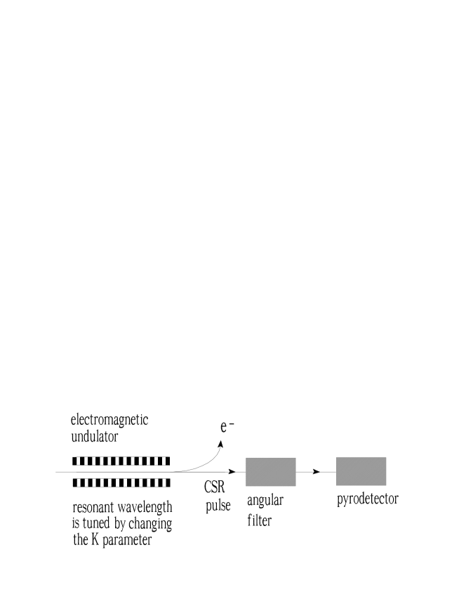
Figure 29: Scheme for electron bunch length diagnostics based on CSR from an undulator

Figure 30: Some typical spectra of the longitudinal electron distribution and undulator spectral distribution function. The bandwidth of the undulator radiation ($\Delta\omega/\omega_{0}=0.89/N_{\mathrm{w}}$) must always be as small as the desired spectral resolution

The principle of operation of the proposed scheme is essentially based on the spectral properties of the undulator radiation. A sample of undulator radiation spectrum at zero angle is shown in Fig. 30. The distribution of the radiated energy within different harmonics depends on the value of $K$. For $K\gg 1$ we will get strong undulator maxima at $\omega=3\omega_{0},\ 5\omega_{0}$ and so forth (as already discussed, the radiation spectrum along the undulator axis includes only odd harmonics). The bunch form factor is the exponential function (3) and the square modulus of bunch form-factor falls off rapidly for wavelengths shorter than the effective bunch length. The fast drop off is evident and for wavelength of about three times shorter than the effective bunch length the radiation power is reduced to about 1 % of the maximum pulse energy at the fundamental harmonic. As a result, sharp changes of the bunch form-factor result in an attenuation of the high undulator harmonics. This point is made clear upon examination of the spectra presented in Fig. 30: actually, the bunch form-factor cut-off affects all higher undulator harmonics which are, therefore, suppressed.

Our goal is to find the relationship between the expected value of radiation energy per pulse and the square modulus of the bunch form-factor. In general, $\mid\bar{F}(\omega)\mid^{2}$ will vary much more slowly in $\omega$ than the sharp resonance term. The two functions might appear as shown in Fig. 30. In such cases, we can replace $\mid\bar{F}(\omega)\mid^{2}$ by the constant value $\mid\bar{F}(\omega_{0})\mid^{2}$ at the center of the sharp resonance curve and take it outside of the integral. What remains is just the integral under the curve of Fig. 28, which is, as we have seen, just equal to (47). Thus, the energy radiated into the central cone by an electron bunch is given by

$$\Delta W_{\mathrm{CSR}}\simeq\frac{\pi e^{2}A_{\mathrm{JJ}}^{2}\omega_{0}K^{2}_{\mathrm{w}}}{c(1+K^{2}_{\mathrm{w}}/2)}N^{2}\mid\bar{F}(\omega_{0})\mid^{2}\ ,$$ (48)

We emphasize the following feature of this result: the CSR radiation energy per pulse is proportional to the square modulus of the bunch form-factor at the resonant frequency. This fact allows one to reconstruct such quantity by repeated measurements of $\Delta W_{\mathrm{CSR}}$ at different resonant frequencies $\omega_{0}$.

4.3 Physical remarks

The typical textbook treatment of the undulator radiation problem (see [3], [8]) consists in finding the expression for the undulator radiation spectrum from (31). However, no attention is usually paid to the region of applicability of this expression. In general this is not correct. In the undulator case, it is important to realize that (31) is valid only when the resonance approximation is met. Naturally, the resonance approximation cannot be expected to be valid when an insertion device has only a few periods. A second important limitation concerns the far field approximation. It is generally assumed that the distance between the undulator and the observer is much larger that the undulator length. This approximation is often assumed without any real justification other than the simplification that results. Such an assumption may or may not be valid, depending on the case.

5 Constrained deconvolution

If both modulus and phase of the bunch form-factor were somehow measured, we would then known the Fourier spectrum of the bunch; an inverse Fourier transform of the measured data $\bar{F}(\omega)$ would then yield the desired profile function $F(t)$ with a resolution limited by the maximum achievable frequency range. Unfortunately, in practice, it is impossible to extract the phase information from the CSR measurement. A more realistic task is to measure the modulus of bunch form-factor only: in Section 4 we proposed a method to perform such a measurement, but independently on the technique selected, the following problem arises, to study what information about the bunch profile can be derived from the collected experimental data: the problem is generally referred to as phase retrieval. There exist some cases in which the absence of phase information is of no consequence. For example, any symmetrical density distribution can be recovered from the knowledge of the form factor modulus only. An example is given by a bunch with a Gaussian density distribution. In practice, the situations in which this assumption is satisfied are probably rather limited.

A possible solution to the loss of phase information was suggested by Wolf [10]. A step forward toward the solution of the problem, is based on the following consideration: if

$$\bar{F}(\omega)=\mid\bar{F}(\omega)\mid\exp\left[\mathop{\mathrm{i}}\phi(\omega)\right]\ ,$$

then

$$\ln\left[\bar{F}(\omega)\right]=\ln\mid\bar{F}(\omega)\mid+\mathop{\mathrm{i}}\phi(\omega)\ .$$

It can be proved that if $\ln\left[\bar{F}(\omega)\right]$ is an analytical function, the phase will be recoverable from the modulus by the relation

$$\phi(\omega)=-\frac{2\omega}{\pi}\int\limits^{\infty}_{0}\frac{\ln\mid\bar{F}(\omega^{\prime})\mid}{(\omega^{\prime})^{2}-\omega^{2}}\mathop{\mathrm{d}}\omega^{\prime}\ .$$

Unfortunately, the analyticity of $\bar{F}(\omega)$ is not a sufficient condition to assure analyticity for $\ln\left[\bar{F}(\omega)\right]$ in that same region. The most obvious reason for this is the possible existence of zeros of $\bar{F}(\omega)$ which lead to singularities in $\ln\left[\bar{F}(\omega)\right]$. In some situation the function $\bar{F}(\omega)$ may have no zeros, in which case the so-called minimum phase solution is valid [11]. However, in general, zeros will be present, and their localization will be unknown a priori.

It should be noticed that, whereas the dispersion relation method is very elegant and conceptually simple, it is not necessarily the ”simplest” method to use in practice. For any given problem, the various possible approaches should be considered, for one may be distinctly easier than another, depending on the problem at hand.

In the particular case of interest, namely an electron bunch originating by the XFEL driver accelerator, we can combine a-priori knowledge about the bunch density distribution with measured information about the bunch form factor. We know that, in the case under examination, the bunching process in zero order approximation can be treated by single particle dynamical theory. We cannot neglect the CSR induced energy spread and other wake fields when we calculate the transverse emittance, but we can neglect them when we calculate the longitudinal current distribution, simply because their contribution to the longitudinal dynamics is small. As a result, we will show that we can define a general temporal structure of the electron bunch after compression without any measurements. The purpose of the measurement is then to determine the numerical value of the parameters on which such temporal structure depends. In this case, sufficient information is provided by the modulus of the bunch form-factor, allowing us to ignore the phase information. The process of finding the best estimate of the profile function $F(t)$ for a particular measured modulus of the bunch form-factor, including utilization of any a priori information available about $F(t)$ refers to a technique called ”constrained deconvolution” which will be exemplified below in detail. Although the context in which the suggestion of this method was made first was spectroscopy [12], the ideas apply equally well in the present context of bunch profile reconstruction.

Let us consider an example which shows the deconvolution process in easy-to-understand circumstances. For emphasis we choose, here, an experiment aimed at measuring the strongly non-Gaussian electron bunch profile at TTF, Phase 2 in femtosecond mode operation. The femtosecond mode operation is based on experience obtained during the operation of the TTF FEL, Phase 1 [6] and it requires one bunch compressor only. An electron bunch with a sharp spike at the head is prepared, with rms width of about 20 microns and a peak current of about one kA. This spike in the bunch generates FEL pulses with duration below one hundred femtoseconds. An example of the longitudinal phase-space distribution for a compressed beam with RF curvature effect is shown in Fig. 31, when the longitudinal bunch charge distribution involves concentration of charges in a small fraction of the bunch length. In the femtosecond mode the first TTF magnetic chicane only will be operational, and this will be the default mode of operation for first lasing.

Figure 31: Typical phase space distribution of electrons after full compression with a single bunch compressor. The plot on the right presents an enlarged fraction of the plot on the left. The head of the bunch is at the left side

Bunch compression for relativistic situations can effectively be achieved, at the time being, only by inducing a correlation between longitudinal position and energy offset with an RF system and taking advantage of the energy dependence of the path length in a magnetic bypass section (a so-called magnetic chicane). In order to study the CSR diagnostic for a compressed bunch, let us first find the longitudinal charge distribution for our bunch model when it is fully compressed by a chicane (here we assume that the perturbation of the bunching process by CSR is negligible). Downstream of the chicane the charge distribution is strongly non-Gaussian with a narrow leading peak and a long tail, as it is seen from the simulation results in Fig. 31. Our attention is focused on determining the longitudinal density distribution after compression. As first was shown in [13] there is an analytical function which provides quite a good approximation for the simulation data. The current distribution along the beam after a single compression is given by

$$I(t)\simeq I_{0}\exp\left(-\frac{t^{2}}{2\tau_{0}^{2}}\right)\qquad{\mathrm{for}}\quad t_{1}>t>-\infty\ ;$$

$$I(t)\simeq\frac{A\exp\left(-t/\tau_{1}\right)}{\sqrt{(t+t_{0})/\tau_{1}}}\qquad{\mathrm{for}}\quad t>t_{1}>0\ .$$ (49)

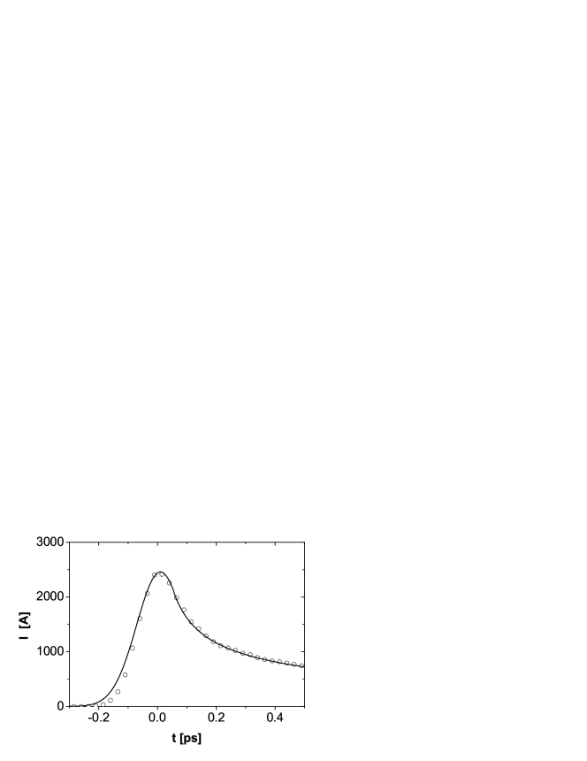
Figure 32: Current distribution along the bunch reconstructed from an ideal set of experimental data for the form-factor and correct value of time constant for the bunch tail (solid curve). Circles present data from a tracking simulation code

Equation (49) gives a good fit. To illustrate how good an approximation to the actual current distribution is provided by (49), we show in Fig. 32 the current as a function of time, first the numerical simulation data, then as computed from (49). Equation (49) involves four independent parameters in the calculation of longitudinal density distribution: $\tau_{0}$, which characterizes the local charge concentration (non-Gaussian feature) of the compressed density, $\tau_{1}$, which characterizes the bunch tail and fitting parameters, $t_{0}$ and $t_{1}$. In this case detailed information on the longitudinal bunch distribution (actually constants: $\tau_{0}$, $\tau_{1}$ and $t_{0}$, $t_{1}$) can be derived from the particular measured square modulus of the bunch form-factor by using an independently obtained tail constant $\tau_{1}$ (for example by means of a streak camera). A quantity of considerable physical interest is the parameter $\tau_{0}$ which characterizes the leading peak. The value of $\tau_{0}$ can be related to the value of the initial local energy spread $\Delta\gamma/\gamma$ in the electron beam if the compaction factor $R_{56}$ of the magnetic chicane is known. Fig. 33 shows plots of the peak current versus time for several values of the local energy spread. By comparing these curves, some feeling can be obtained about the effective reduction in peak current. As the energy spread is increased from 5 keV to 15 keV, the maximum peak current falls from 3.5 kA to 2 kA.

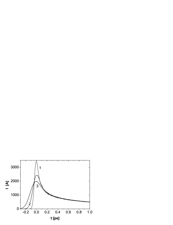
Figure 33: Typical current distribution along the bunch after full compression with a single bunch compressor. Curve 1, 2, and 3 correspond to local energy spread of 5, 10, and 15 keV at the entrance of the bunch compressor. The head of the bunch is at the left side. The charge of the bunch is 3 nC

The highest time resolution obtainable by means of a streak camera is in the sub-picosecond range. By means of coherent radiation, the resolution can be made comparatively high because the resolution is determined by the spectral range in the measurement. Hence, this method will be useful for monitoring an ultra-short electron bunch at TTF FEL. In the TTF FEL Phase 2 the measurement of CSR spectrum can be made by using long period electromagnetic undulator as shown in Fig. 34. As already said, for the complete determination of the bunch profile function, downstream of the first TTF FEL bunch compressor, a measurement of the bunch length can be made independently by using a sub-picosecond resolution streak camera. The limiting resolution of the streak camera will prevent the measurement of the spike width. Nevertheless, the streak camera can detect the long time tail which is outside the CSR detector response.

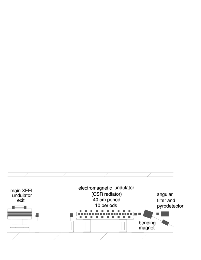
Figure 34: Bunch length measurement scheme for TTF XFEL. The CSR source uses the spent electron beam coming from the XFEL

The significance of the proposed scheme cannot be fully appreciated until we determine typical values of the energy in the radiation pulse detected within the central cone that can be expected in practice. In the case of TTF FEL, the bunch form factor modulus falls off rapidly for wavelengths shorter than 40 microns. At the opposite extreme, the dependence of the form factor on the exact shape of the electron bunch is rather weak and can be ignored outside the wavelength range $40\mu{\mathrm{m}}<\lambda<100\mu{\mathrm{m}}$. This point is made clear upon examination of the curves presented in Fig. 35. The energy in the radiation pulse can be estimated simply as in (48). From Fig. 36 it is quite clear that in the $40\mu{\mathrm{m}}-100\mu{\mathrm{m}}$ wavelength region of the CSR spectrum any local energy spread in the electron beam smaller than 20 keV produces energies larger than $0.1\mu{\mathrm{J}}$ in the radiation pulse.

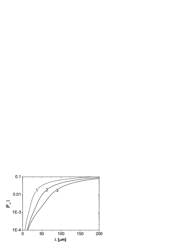
Figure 35: Form-factor of the electron bunch corresponding to the bunch profiles shown in Fig. 33

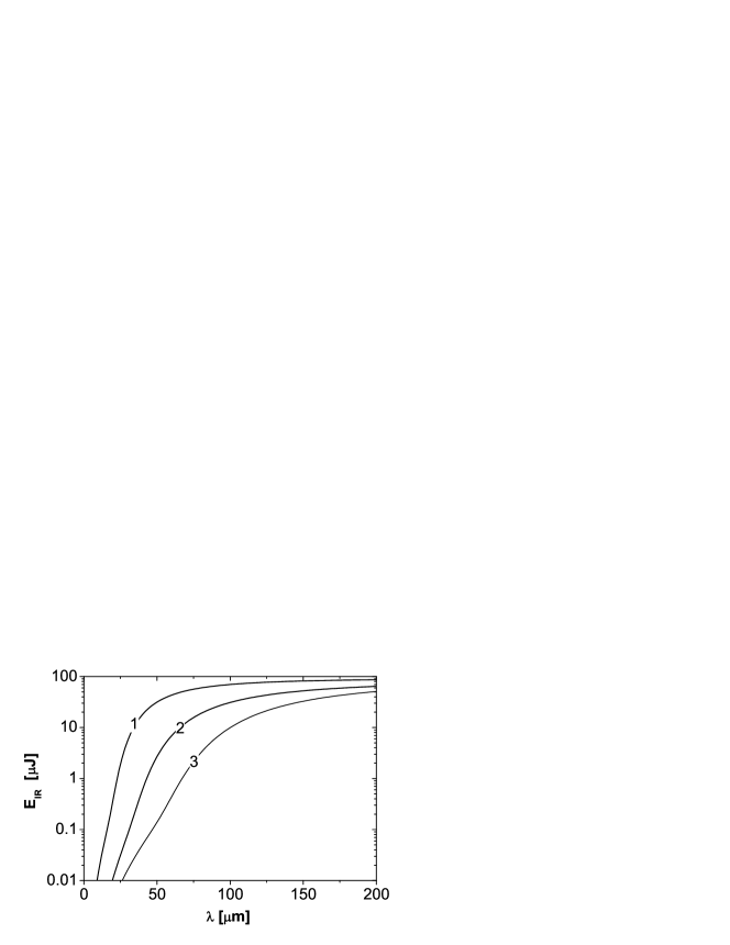
Figure 36: Energy in the radiation pulse detected within central cone. Curves 1, 2, and 3 correspond to a local energy spread of 5, 10, and 15 keV at the entrance to the bunch compressor (see Fig. 33). The bunch charge is 3 nC

To conclude this section we present examples of deconvolution of computer generated data; we hope that these will provide useful insight into the practical limits of deconvolution. We will demonstrate that constrained deconvolution is a useful experimental tool testable at each step in its development. By far the easiest and most informative way to examine the deconvolution process is to use a computer in place of a CSR spectrometer. By simulating a spectrum rather than using an actual CSR spectrometer to record it, we have a complete control over such factors as resolution, shape and noise. Also, we know what the perfectly deconvolved profile function would look like. In the deconvolution of actual CSR spectral data, the presence of noise is usually the main limiting factor: the effects of noise on deconvolution are demonstrated in the following. For the purpose of examining the deconvolution process, we begin with noisy data, which of course, can be realized in a simulation process. When other aspects of deconvolution, such as errors in the prior information are examined, noiseless data are used.

Figure 37: Electron bunch form factor corresponding to the case of 10 keV energy spread at the entrance of the bunch compressor. The solid curve presents an ideal measurement. Symbols present five sets of measurements with relative error $\pm 40\%$

Figure 38: Current distribution reconstructed from five sets of measurements with relative error $\pm 40\%$ (see Fig. 37). The solid line corresponds to an ideal measurement. The tail time constant in all cases is 9 ps

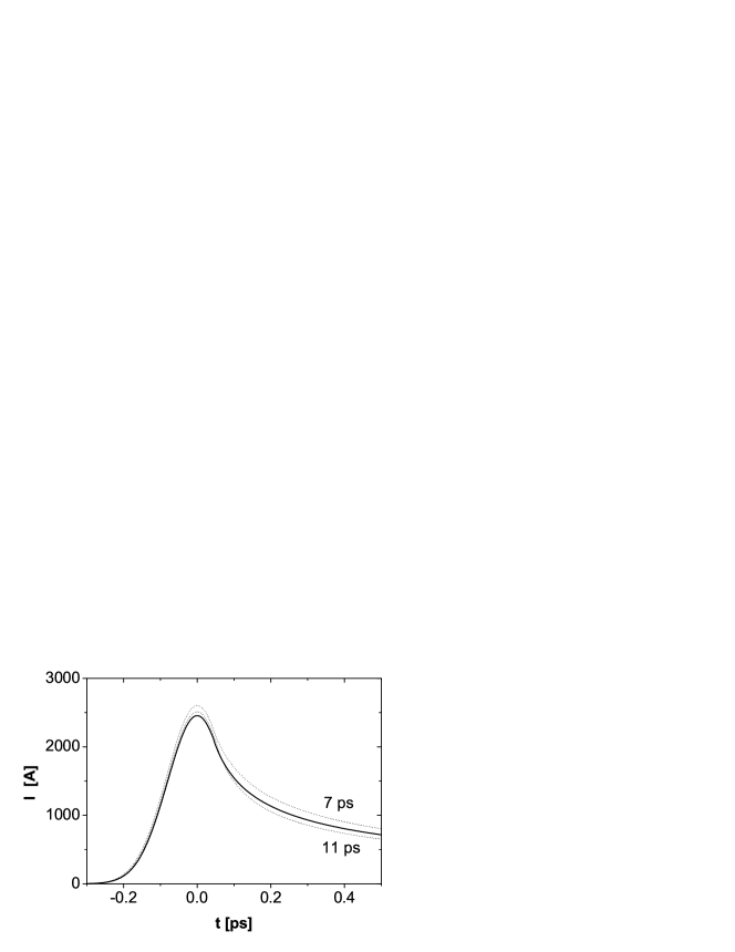
Figure 39: Current distribution reconstructed from an ideal set of experimental data for the form-factor (see Fig. 37), but with different values of time constants, 7 and 11 ps, for the bunch tail (dotted lines). The solid line corresponds to the correct value of the time constant, 9 ps

Our goal is to discover the limiting sensitivity of the measurement technique considered. Attention is therefore turned to the crucial question of how accurately the bunch profile parameters can be measured by this technique when the errors in the input data cannot be neglected. Surely, the preferable way to answer the question about errors in bunch form-factor measurement is the computer experiments way. The effects of various errors are included in a full simulation of deconvolution procedure. One important question to answer is about how well the modulus of bunch form factor must be known in order to perform a successful deconvolution. To obtain the sensitivity to error effects, we use a set of input error data for a simulated bunch profile spectrum (see Fig. 37). A 40% rms error (variable over the undulator scan) is included. The sensitivities of the final bunch profile function to the simulation input errors are summarized in Fig. 38. Only one random seed has been presented here as an example, but several seeds have been run with similar success. Fig. 38 shows that rms of CSR measurement should be within $\pm 50\%$. It is seen that the constrained deconvolution method is insensitive to the errors in the bunch form-factor.

As shown above, the bunch profile function is given by (49). An important issue to deal with consists in determining the dependence of the deconvolved function on the tail constant. One way to investigate this matter is to use a set of tail constants which differ from the real one in the deconvolution of a simulated spectrum. Fig. 39 shows the results of such a test. At first glance all three traces of Fig. 39 are practically identical, indicating that the tail parameter is less important than it would have probably been expected. We can therefore conclude that the width of the tail parameter should be within $\pm 50\%$ of the proper value. However, if the correct tail function is not readily determined (by a streak camera) there is some justification for deconvolution with a ”good guess” because even the extreme case shown in Fig. 39 is superior to trace the profile function without prior information.

6 Concluding remarks

Electron pulse-shape measurement is achieved by a three-step process.

(i) In the first step spectrum of coherent radiation $P(\omega)$ is measured. Coherent radiation from dipole magnet is emitted over a wide spectrum and should be analyzed with a spectrometer or interferometer. The proposed technique of using CSR from an undulator may be a more promising approach. The basic measurement in this case is extremely simple: the energy of the coherent radiation pulse within the central cone is recorded by a bolometer. In order to use the radiation from the undulator it has to be filtered: for such a purpose, a simple pinhole can be used.

(ii) The second step is to deduce the modulus of the bunch form-factor from the equation $P(\omega)=p(\omega)N^{2}\mid\bar{F}(\omega)\mid^{2}$; $p(\omega)$ should be applied to the result of the measurement, to obtain the bunch form factor. A careful analysis of the diagnostic instrumentation is required to find its exact $p(\omega)$ function. The computation of the single-particle spectrum for practical accelerator applications is a rather difficult problem. The long wavelength synchrotron radiation from bending magnets in the near zone integrates over many different vacuum chamber pieces and the quantity $p(\omega)$ is usually very difficult to know with good accuracy within the long wavelength range. In principle, modern computers allow one to perform direct calculation of the factor $p(\omega)$. The results of such simulations will depend on a large number of parameters. They will provide the possibility of obtaining a numerical answer for a specific set of input data, but hardly help to understand the physics of the problem. Success come to those who start from the physical point of view and begin by making the right kind of approximations, knowing what is large and what is small in a given complicated situation. We hope that the simple model employed here offers a useful introduction to the more formidable problems which arise in the computation of spontaneous emission spectrum distortions for real accelerators.

(iii) The third step consists in the reconstruction of the electron bunch profile from the measured data. The CSR spectrum measurement has an important limitation: it does not provide any information on the phase content of the pulse. It is clear that the retrievability of the information about the electron bunch profile function will in general not be complete, for it is the particular measured square modulus of the form-factor that can be obtained, not the complex form-factor itself. No spectral phase information is available, and the complete profile function cannot be obtained in general. Nevertheless, the less complete information can be exceedingly useful in many cases. For example, downstream of the bunch compressor the bunch charge distribution is strongly non-Gaussian with a narrow leading peak and a long tail. In this case detailed information about the longitudinal bunch distribution can be derived from the measured square modulus $\mid\bar{F}(\omega)\mid^{2}$ by measuring the bunch tail constant with a streak camera and by using all a-priori available information about profile function. In this paper we demonstrate that constrained deconvolution is a useful experimental tool testable at each step in its development. Although the present work is concerned primarily with fully compressed electron bunch downstream of the first bunch compressor, its applicability is not restricted to that area only: for example, multistage bunch compression is a suitable candidate for treatment by the methods described here.

References

- [1] TESLA Technical Design Report, DESY 2001-011, edited by F. Richard et al., and http://tesla.desy.de/
-
[2]
The LCLS Design Study Group, LCLS Design Study Report, SLAC reports
SLAC- R521, Stanford (1998) and
http:
www-ssrl.slacstanford.edu/lcls/CDR - [3] H. Wiedemann, ”Particle Accelerator Physics” (Springer, Berlin, 1995)
- [4] J. Schwinger, Phys. Rev. 75, 1912 (1949)
- [5] V. G Bagrov, N. I. Fedosov, and I. M. Ternov, Phys. Rev. D 28, 2464 (1982)
- [6] V. Ayvazyan et al., Phys. Rev. Lett. 88(2002)104802
- [7] J. D. Jackson, ”Classical electrodynamics” (John Wiley and Sons, New York, 1975)
- [8] P. J. Duke, ” Synchrotron radiation” (Oxford University Press, Oxford, 2000)
- [9] V. A. Bordovitsyn (Editor), ”Synchrotron Radiation Theory And Its Development” (World Scientific, Singapure-London, 1999)
- [10] E. Wolf, Proc. Phys. Soc., 80, 1269 (1962)
- [11] S. R. Robinson, J. Opt. Soc. Am., 68, 87 (1978)
- [12] P. A. Jansson (Editor), ”Deconvolution with application in spectroscopy” Academic Press, Inc. (1984)
- [13] R. Li, Nucl. Instr. and Meth. A 475(2001)498