Electromagnetic energy-momentum and forces in matter

Abstract

We discuss the electromagnetic energy-momentum distribution and the mechanical forces of the electromagnetic field in material media. There is a long-standing controversy on these notions. The Minkowski and the Abraham energy-momentum tensors are the most well-known ones. We propose a solution of this problem which appears to be natural and self-consistent from both a theoretical and an experimental point of view.

I Introduction

The discussion of the energy-momentum tensor in macroscopic electrodynamics is quite old. The beginning of this dispute goes back to Minkowski [1], Abraham [2], and Einstein and Laub [3]. Good reviews of the problem can be found in [4, 5, 6, 7], to mention but a few. Nevertheless, up to now the question was not settled and there is an on-going exchange of conflicting opinions concerning the validity of the Minkowski versus the Abraham energy-momentum tensor, see [8] for a recent discussion. Even experiments were not quite able to make a definite and decisive choice of electromagnetic energy and momentum in material media.

Here we propose the solution of the problem.

Our basic notations and conventions are as follows. We are using international SI units throughout. Correspondingly, $\varepsilon_{0},\mu_{0}$ are the electric and the magnetic constant (earlier called vacuum permittivity and vacuum permeability). The Minkowski metric is $g_{ij}={\rm diag}(c^{2},-1,-1,-1)$. Latin indices from the middle of the alphabet label the spacetime components, $i,j,k,\dots=0,1,2,3$, whereas those from the beginning of the alphabet refer to 3-space: $a,b,c,\dots=1,2,3$.

II New energy-momentum tensor

Our solution is as follows. The new electromagnetic energy-momentum in an arbitrary medium reads:

$$\mu_{0}\,T_{i}{}^{j}=-\,F_{ik}\,F^{jk}+{\frac{1}{4}}\,\delta_{i}^{j}\,F_{kl}F^{kl}.$$ (1)

The electromagnetic field strength $F_{ij}=({\bf E},{\bf B})$ is composed of the electric and magnetic 3-vector fields. Componentwise, Eq.(1) describes the energy density of the field

$$T_{0}{}^{0}=u={\frac{1}{2}}\left(\varepsilon_{0}\,E^{2}+{\frac{1}{\mu_{0}}}\,B^{2}\right),$$ (2)

its energy flux density (or Poynting vector)

$$T_{0}{}^{a}=s^{a}={\frac{1}{\mu_{0}}}\,\left[{\bf E}\times{\bf B}\right]^{a},$$ (3)

its field momentum density

$$T_{a}{}^{0}=-\,p_{a}=\varepsilon_{0}\,\left[{\bf B}\times{\bf E}\right]_{a},$$ (4)

and the Maxwell stress tensor

$$T_{a}{}^{b}=S_{a}{}^{b} = \varepsilon_{0}\left(E_{a}E^{b}-{\frac{1}{2}}\,\delta_{a}^{b}\,E^{2}\right)$$ (6)

$$\quad+{\frac{1}{\mu_{0}}}\left(B_{a}B^{b}-{\frac{1}{2}}\,\delta_{a}^{b}\,B^{2}\right).$$

As one can immediately notice that (1) has the same form as the vacuum energy-momentum tensor. However, its physical content is different, which follows from the fact that $F_{ij}=({\bf E},{\bf B})$ satisfies the macroscopic Maxwell equations in matter:

$$\nabla\times{\bf H}-\dot{\bf D} = {\bf j}^{\rm free},\qquad\nabla\cdot{\bf D}=\rho^{\rm free},$$ (7)

$$\nabla\times{\bf E}+\dot{\bf B} = 0,\qquad\nabla\cdot{\bf B}=0.$$ (8)

Here $\rho^{\rm free}$ and ${\bf j}^{\rm free}$ are the densities of the free (or, in other terminology, the “true” or “external”) charge and the free current. The fields ${\bf D}$ and ${\bf H}$ represent the electric and magnetic excitations (other names are “electric displacement” and “magnetic field intensity”). The field strengths $({\bf E},{\bf B})$ and the excitations $({\bf D},{\bf H})$ are related by means of the equations

$$\varepsilon_{0}\,{\bf E}={\bf D}-{\bf P},\quad{\rm and}\quad{\frac{1}{\mu_{0}}}\,{\bf B}={\bf H}+{\bf M}.$$ (9)

The polarization ${\bf P}$ and the magnetization ${\bf M}$ represent the bound (or “polarizational”) current and charge densities inside the material medium:

$${\bf j}^{\rm mat}=\dot{\bf P}+\nabla\times{\bf M},\qquad\rho^{\rm mat}=-\,\nabla\cdot{\bf P}.$$ (10)

The density of the mechanical (ponderomotive) force acting on matter is determined as the divergence of the energy-momentum tensor

$$f_{i}=\partial_{j}\,T_{i}{}^{j}.$$ (11)

Differentiating (1) and using the Maxwell equations (7), (8) and the equations (9) and (10), yields:

$$f_{0} = \dot{u}+\nabla\cdot{\bf s}=-\,{\bf E}\cdot{\bf j}^{\rm tot},$$ (12)

$$f_{a} = -\,\dot{p}_{a}+\partial_{b}\,S_{a}{}^{b}=\rho^{\rm tot}\,E_{a}+\left[{\bf j}^{\rm tot}\times{\bf B}\right]_{a}.$$ (13)

Here the total charge and current density are $\rho^{\rm tot}=\rho^{\rm free}+\rho^{\rm mat}$ and ${\bf j}^{\rm tot}={\bf j}^{\rm free}+{\bf j}^{\rm mat}$.

This result is quite natural and physically clear. The electromagnetic field affects matter by means of the two Lorentz forces (13): One acts on the free charge and current $(\rho^{\rm free},{\bf j}^{\rm free})$ (on the conductive current, for example), and another force acts on the bound charge and current (10). The latter have also a direct physical meaning in the macroscopic (Lorentz type averaging) framework and in the microscopic approaches, see Hirst [9], e.g. The temporally and spatially varying polarization and magnetization give rise to the electric and magnetic fields, like the free charges and currents do. Conversely, the bound charges and currents should also feel the electromagnetic field in the same way as the free charges and currents do.

The representation of the total electromagnetic force as the sum of the two terms with the clear-cut physical content (13) suggests a natural step to split the original energy-momentum (1) into the corresponding sum of the two energy-momentum tensors which are associated with the free and bound charge/current, respectively. Using (9) in (1), we find

$$T_{i}{}^{j}={}^{\rm f}T_{i}{}^{j}+{}^{\rm b}T_{i}{}^{j},$$ (14)

where we introduce the free-charge energy-momentum and the bound-charge energy-momentum tensors as

$${}^{\rm f}T_{i}{}^{j}=\left(\begin{array}[]{c|c}{}^{\rm f}u&-\,{}^{\rm f}p_{a}\\ \hline\cr{}^{\rm f}s^{b}&{}^{\rm f}S_{a}{}^{b}\end{array}\right),\qquad{}^{\rm b}T_{i}{}^{j}=\left(\begin{array}[]{c|c}{}^{\rm b}u&-\,{}^{\rm b}p_{a}\\ \hline\cr{}^{\rm b}s^{b}&{}^{\rm b}S_{a}{}^{b}\end{array}\right).$$ (15)

The components of the free-charge energy-momentum read explicitly

$${}^{\rm f}u = {\frac{1}{2}}\left({\bf E}\cdot{\bf D}+{\bf B}\cdot{\bf H}\right),$$ (16)

$${}^{\rm f}{\bf s} = {\bf E}\times{\bf H},\qquad{}^{\rm f}{\bf p}={\bf D}\times{\bf B},$$ (17)

$${}^{\rm f}S_{a}{}^{b} = E_{a}D^{b}+B_{a}H^{b}-{\frac{1}{2}}\,\delta_{a}^{b}\left({\bf E}\cdot{\bf D}+{\bf B}\cdot{\bf H}\right),$$ (18)

whereas the components of the bound-charge energy-momentum are

$${}^{\rm b}u = {\frac{1}{2}}\left(-\,{\bf E}\cdot{\bf P}+{\bf B}\cdot{\bf M}\right),$$ (19)

$${}^{\rm b}{\bf s} = {\bf E}\times{\bf M},\qquad{}^{\rm b}{\bf p}=-\,{\bf P}\times{\bf B},$$ (20)

$${}^{\rm b}S_{a}{}^{b} = -\,E_{a}P^{b}+B_{a}M^{b}-{\frac{1}{2}}\,\delta_{a}^{b}\left(-\,{\bf E}\cdot{\bf P}+{\bf B}\cdot{\bf M}\right).$$ (21)

One straightforwardly recognizes the tensor ${}^{\rm f}T_{i}{}^{j}$ with the components (16)-(18) as the well-known Minkowski energy-momentum tensor.

Similarly to (11), the divergences ${}^{\rm f}f_{i}=\partial_{j}{}^{\rm f}T_{i}{}^{j}$ and ${}^{\rm b}f_{i}=\partial_{j}{}^{\rm b}T_{i}{}^{j}$ determine the force densities. By construction, the total 4-force density is the sum $f_{i}={}^{\rm f}f_{i}+{}^{\rm b}f_{i}$. Explicitly, we have for the 3-force densities

$${}^{\rm f}f_{a} = \rho^{\rm free}\,E_{a}+\left[{\bf j}^{\rm free}\times{\bf B}\right]_{a}-X_{a},$$ (22)

$${}^{\rm b}f_{a} = \rho^{\rm mat}\,E_{a}+\left[{\bf j}^{\rm mat}\times{\bf B}\right]_{a}+X_{a}.$$ (23)

Here, in the Cartesian coordinates,

$$X_{a}={\frac{1}{2}}\left(E^{b}\partial_{a}D_{b}-D^{b}\partial_{a}E_{b}+H^{b}\partial_{a}B_{b}-B^{b}\partial_{a}H_{b}\right).$$ (24)

In particular, $X_{a}=\!{\frac{1}{2}}\!\left[\varepsilon_{0}\,E_{b}E_{c}\partial_{a}\varepsilon^{bc}+\mu_{0}\,H_{b}H_{c}\partial_{a}\mu^{bc}\right]$ for the linear material laws $D^{a}=\varepsilon_{0}\,\varepsilon^{ab}E_{b}$ and $B^{a}=\mu_{0}\,\mu^{ab}H_{b}$. This extra term vanishes for homogeneous media.

Thus indeed, tensors in the sum (14) are associated with the two different types of charges and currents in the material medium. The divergences produce, essentially, the two independent Lorentz forces acting separately on the free and on the bound charge and current.

III Some properties and applications

After all these preliminaries and formal derivations, we are in a position to discuss the physical properties of the energy-momentum (1). At first, some remarks about (1) in comparison to the Minkowski and Abraham tensors. Many authors (see the discussions in [5, 6, 7]) pointed to a clearly unphysical result produced by the Minkowski energy-momentum: in the absence of free charges and currents, a homogeneous medium appears to be always subject to the zero electromanetic force. This fact was usually taken in favor of the Abraham tensor which predicts an extra, so called Abraham force. However, the energy-momentum (1) does not suffer from such a deficiency. Even when the free charge and current densities are vanishing, the total force is, in general, non-trivial in view of the presence of polarization charge and current. Moreover, as compared to the rather ad hoc choice of the Abraham force, the mechanical action on the bound charge and current is in all cases described, using (1), by the well-known Lorentz force (13).

Furthermore, the Minkowski tensor is asymmetric which is obvious from the comparison of the energy flux ${}^{\rm f}{\bf s}$ and the field momentum ${}^{\rm f}{\bf p}$ in (17). Usually, this fact was also taken in favor of the Abraham tensor, which is symmetric. At the same time, despite its symmetry, the structure of the Abraham tensor is defined in a rather ad hoc manner with opaque physical motivations. In contrast to this, the energy-momentum (1) is naturally symmetric and the electromagnetic field momentum (4) is related to the energy flux (3) as ${\bf p}={\bf s}/c^{2}$. This is the famous Planck relation which generalizes the Einsteinian $\Delta m=\Delta E/c^{2}$ relation to field theory. The interesting discussion of von Laue [10] was concentrated mainly around this point.

As a simple application, let us consider the propagation of an electromagnetic plane wave from the vacuum into a dielectric medium with $\mu=1$ and refractive index $n=\sqrt{\varepsilon}$. More exactly, like in the previous discussions [11, 6, 7], we will confine ourselves to the case of a gaseous medium consisting of heavy atoms. We assume normal incidence on a plane boundary and we recall the reflection and transmission coefficients $R=(n-1)/(n+1)$ and $T=2/(n+1)$, respectively. Then, for incident and reflected waves in vacuum, we find for the mean field energy (16) and momentum (17), if averaged over one period,

$$\overline{u} = \varepsilon_{0}\,{\frac{|E_{0}|^{2}}{2}}\,(1+R^{2})=\varepsilon_{0}\,|E_{0}|^{2}\,{\frac{1+n^{2}}{(1+n)^{2}}},$$ (25)

$$\overline{\bf p} = {\frac{\varepsilon_{0}}{c}}\,{\frac{|E_{0}|^{2}}{2}}\,(1-R^{2})\,{\bf k}={\frac{\varepsilon_{0}}{c}}\,|E_{0}|^{2}\,{\frac{2n}{(1+n)^{2}}}\,{\bf k}.$$ (26)

On the other hand, within the dielectric, for the transmitted wave, Eqs. (16), (19) and (17), (20) yield

$$\overline{u} = \varepsilon_{0}\,{\frac{1+n^{2}}{2}}\,{\frac{|E_{0}|^{2}}{2}}\,T^{2}=\varepsilon_{0}\,|E_{0}|^{2}\,{\frac{1+n^{2}}{(1+n)^{2}}},$$ (27)

$$\overline{\bf p} = {\frac{\varepsilon_{0}n}{c}}\,{\frac{|E_{0}|^{2}}{2}}\,T^{2}\,{\bf k}={\frac{\varepsilon_{0}}{c}}\,|E_{0}|^{2}\,{\frac{2n}{(1+n)^{2}}}\,{\bf k}.$$ (28)

Here $E_{0}$ is the amplitude of the electric field and ${\bf k}$ the unit wave vector which specifies the direction of propagation. Comparing the above formulas, we see that both, the total energy and the total momentum calculated on the basis of (1), are conserved on the passage of the wave into the medium. This conclusion is in a complete agreement with the previous studies [11, 6, 7]. Moreover, it can be supplemented by a far more detailed analysis of wave propagation in a gaseous media that has demonstrated [11, 6, 7] the plausibility of the (“Abraham”) field momentum ${\bf E}\times{\bf H}/c$. However, since all these studies were confined to dielectrics with $\mu=1$, the arguments presented in [11, 6, 7] in actual fact give support to the field momentum (4) likewise.

IV Walker and Walker experiment

Finally, let us discuss the direct experimental confirmations of the energy-momentum (1). For this purpose, as a first example, we recall the measurements of Walker & Walker [12] of the force acting on a dielectric disk placed in crossed oscillating electric and magnetic fields, see Fig.1(a). The scheme of the experiment is as follows: The symmetry of the problem suggests to use cylindrical coordinates $(r,\varphi,z)$. A small cylinder is made of barium titanate with $\varepsilon=3340$ and $\mu=1$. Its height in $z$-direction is $l\approx 2$ cm, internal radius $r_{1}\approx 0.4$ cm, and external radius $r_{2}\approx 2.6$ cm. This disk is suspended between the poles of an electromagnet which creates the harmonically oscillating axial magnetic field. Besides, the oscillating field, with the phase difference of $\pi/2$, a radial electric field is created by means of an alternating voltage applied between the inner and the outer cylindrical surfaces of the disk. The oscillation frequency of the fields is rather low, namely, $\omega=60$ Hz. As a consequence, everywhere in the disk $r\omega n/c\sim z\omega n/c\sim 10^{-7}\ll 1$. Walker & Walker [12] measured the torque around the $z$-axis produced by the electromagnetic force.

Let us derive the theoretical value of the torque which is given by the volume integral

$$N_{z}=\int_{\rm disk}dv\,[{\bf r}\times{\bf f}]_{z}=\int_{\rm disk}dv\,rf_{\varphi}.$$ (29)

Since there are no free charges and currents in the dielectric, the Lorentz force (13) reduces only to the second term determined by the bound charges and currents. One can check that the Maxwell equations (7), (8), together with the constitutive relations ${\bf D}=\varepsilon\varepsilon_{0}{\bf E}$ and ${\bf B}=\mu_{0}{\bf H}$, are solved by the electric and magnetic field configuration

$${\bf E} = \sin(\omega t)\left({\frac{U_{0}}{r\log(r_{2}/r_{1})}}\,{\bf e}_{r}+{\frac{B_{0}}{2}}\,\omega r\,{\bf e}_{\varphi}\right),$$ (30)

$${\bf B} = \cos(\omega t)\left(B_{0}\,{\bf e}_{z}-{\frac{\varepsilon U_{0}}{r\log(r_{2}/r_{1})\,c^{2}}}\,\omega z\,{\bf e}_{\varphi}\right).$$ (31)

These approximate formulas are valid with very high accuracy due to the fact that $r\omega n/c\sim z\omega n/c\sim 10^{-7}\ll 1$ everywhere in the disk. As usual, $({\bf e}_{r},{\bf e}_{\varphi},{\bf e}_{z})$ denote the local orthonormal frame vectors of the cylindrical coordinate system. Here $B_{0}$ is the magnitude of the oscillating axial magnetic field and $U_{0}$ is the amplitude of the voltage applied between the inner ($r=r_{1}$) and the outer ($r=r_{2}$) cylindrical surfaces of the disk, $\Delta U=U_{0}\,\sin(\omega t)$.

The bound charge and current densities (10) are straightforwardly found to be $\rho^{\rm mat}=0$ and ${\bf j}^{\rm mat}=\dot{\bf P}=\varepsilon_{0}(\varepsilon-1)\dot{\bf E}$. Correspondingly, the Lorentz force turns out to be ${\bf f}={\bf j}^{\rm mat}\times{\bf B}=\varepsilon_{0}(\varepsilon-1)\dot{\bf E}\times{\bf B}$. Substituting (30) and (31) in (29), we obtain the torque

$$N_{z}=-\,\varepsilon_{0}(\varepsilon-1)\,\pi\,l\,(r_{2}^{2}-r_{1}^{2})\,{\frac{U_{0}B_{0}\omega}{\log(r_{2}/r_{1})}}\,\cos^{2}(\omega t).$$ (32)

This result was experimentally confirmed by Walker & Walker [12]. Although the authors of [12] apparently noticed that the torque measured fits the understanding of the electromagnetic force as the Lorentz force for the polarization current (in agreement with our approach), they ultimately claimed that their experiment confirms the Abraham force. The theoretical explanation presented in [12] was based on the idea that the Maxwell stress $S_{a}{}^{b}$ caused the unusual surface drag of the disk. However, when computing the force, see (13), the contribution of the stress $\partial_{b}\,S_{a}{}^{b}$ should be complemented by the momentum term $-\,\dot{p}_{a}$; the latter is missing in [12]. The alternative explanation [5] is based on the computation of forces on the metal coatings of the cylinder. This yields the result where the factor $(\varepsilon-1)$ above is replaced by $\varepsilon$. Since the dielectric matter in question has $\varepsilon=3340$, this experiment thus cannot be treated as the critical test for the different energy-momenta.

V Experiment of James

As another example we consider the experiment of James [13] which is in many respects very similar to the one of Walker & Walker. James, see Fig.1(b), had also placed a disk into crossed electric and magnetic fields. The small cylinders were made of a composition of nickel-zinc ferrite with $\mu=16$ or $43$ and $\varepsilon\approx 7$. Like in [12], the radial electric field was created by means of an oscillating voltage applied between the inner and the outer cylindrical surface of the disk. However, instead of an axial magnetic field, an azimuthal magnetic field was produced inside matter by an alternating electric current in a conducting wire placed along the axis of the disk. The resulting field configuration reads:

$${\bf E} = \left({\frac{U_{0}\,\sin(\omega_{u}t)}{r\log(r_{2}/r_{1})}}-{\frac{\mu\mu_{0}I_{0}}{2\pi r}}\,\cos(\omega_{i}t)\,\omega_{i}z\right){\bf e}_{r},$$ (33)

$${\bf B} = \left({\frac{\mu\mu_{0}I_{0}}{2\pi r}}\,\sin(\omega_{i}t)-{\frac{\mu\varepsilon\,U_{0}\,\cos(\omega_{u}t)}{r\log(r_{2}/r_{1})\,c^{2}}}\,\omega_{u}z\right){\bf e}_{\varphi}.$$ (34)

These formulas hold true in the approximation $z\omega_{u}n/c\sim z\omega_{i}n/c\sim 10^{-5}\ll 1$ which is fulfilled in James’ experiment everywhere in the cylinders with $r_{1},r_{2}$ and the length $l$ of order 1-3 centimeter. Here $I_{0}$ is the amplitude of the alternating current $I=I_{0}\,\sin(\omega_{i}t)$ along the $z$-axis, whereas $U_{0}$ gives, as before, the amplitude of the oscillating voltage, $\Delta U=U_{0}\,\sin(\omega_{u}t)$. The frequencies $\omega_{i}$ and $\omega_{u}$ are different and are varied in the course of the experiment between 10 and 30 kHz. Since this experiment, unlike [12], covers also magnetic media, we display the nontrivial permeability $\mu$. One can check that (33), (34) satisfy the Maxwell equations (7), (8).

A Electromagnetic force in James’ experiment

James [13] measured the force ${\cal F}_{z}$ acting along the axis of the disk in the crossed fields (33), (34). Let us derive the theoretical value of this force by using the general expression for the force density (13). There are no free charges and currents inside matter, $\rho^{\rm free}=0$ and ${\bf j}^{\rm free}=0$. By substituting (33), (34) into (10), we find $\rho^{\rm mat}=0$ and

$${\bf j}^{\rm mat}=\varepsilon_{0}\,(\mu\varepsilon-1)\Bigg{(}{\frac{\omega_{u}\,U_{0}\,\cos(\omega_{u}t)}{r\log(r_{2}/r_{1})}}+{\frac{\mu\mu_{0}I_{0}}{2\pi r}}\,\sin(\omega_{i}t)\,\omega_{i}^{2}z\Bigg{)}{\bf e}_{r}.$$ (35)

The total force is obtained as the integral of the force density

$${\bf j}^{\rm mat}\times{\bf B} = {\frac{(\varepsilon\mu-1)\varepsilon_{0}}{r^{2}}}\Big{[}{\frac{\mu\mu_{0}\,U_{0}I_{0}}{2\pi\log(r_{2}/r_{1})}}\,\omega_{u}\,\sin(\omega_{i}t)\cos(\omega_{u}t)$$ (37)

$$-\,\left(nU_{0}/c\log(r_{2}/r_{1})\right)^{2}\,\omega_{u}^{2}\,\cos^{2}(\omega_{u}t)\,z+(\mu\mu_{0}I_{0}/2\pi)^{2}\,\omega_{i}^{2}\,\sin^{2}(\omega_{i}t)\,z\Big{]}\,{\bf e}_{z}$$

over the volume of the disk:

$${\cal F}_{z}=\int_{\rm disk}dv\,[{\bf j}^{\rm mat}\times{\bf B}]_{z}={\frac{(\mu\varepsilon-1)\mu lU_{0}I_{0}}{c^{2}}}\,\omega_{u}\,\sin(\omega_{i}t)\cos(\omega_{u}t).$$ (38)

According to James [13], we choose $\omega_{i}=\omega_{u}\pm\omega_{0}$, with $\omega_{0}$ the mechanical resonance frequency of the disk, and find the final expression for the force

$${\cal F}_{z}=\pm\,{\frac{(\mu\varepsilon-1)\mu lU_{0}I_{0}}{2c^{2}}}\,\omega_{u}\,\sin(\omega_{0}t).$$ (39)

This theoretical prediction was actually verified in the experiment of James [13].

B Minkowski and Abraham forces in James’ experiment

In the isotropic case under consideration, $\varepsilon^{ab}=\delta^{ab}\,\varepsilon$ and $\mu^{ab}=\delta^{ab}\,\mu$. With the free charges and currents absent, the Minkowski 3-force density (22) reduces to the last term which contributes only at the ends of the cylinder. Since the permittivity has the constant value of $\varepsilon\neq 1$ inside the body, i.e. for $-l/2<z<l/2$, and drops to $\varepsilon=1$ outside of that interval, the derivative of such a stepwise function reads $\partial_{z}\varepsilon(z)=(\varepsilon-1)\left[\delta(z+l/2)-\delta(z-l/2)\right]$. Similar relation holds for the derivative of the permeability function $\mu(z)$. Correspondingly, we find for the Minkowski force

$${\cal F}_{z}^{\rm M} = -\,\int_{\rm disk}dvX_{z}=-\,{\frac{1}{2}}\int_{\rm disk}dv\left[\varepsilon_{0}\,E^{2}\,\partial_{z}\varepsilon+\mu_{0}\,H^{2}\,\partial_{z}\mu\right]$$ (40)

$$= \pi\int_{r_{1}}^{r_{2}}dr\,r\left\{(\varepsilon-1)\varepsilon_{0}\left[E^{2}(l/2)-E^{2}(-l/2)\right]+(\mu-1)\mu_{0}\left[H^{2}(l/2)-H^{2}(-l/2)\right]\right\}.$$ (41)

Substituting the squares of the electric and magnetic fields (33) and (34) [note that ${\bf H}={\bf B}/\mu\mu_{0}$], we obtain:

$${\cal F}_{z}^{\rm M}=-\,{\frac{l\,U_{0}I_{0}}{c^{2}}}\left[\mu(\varepsilon-1)\,\omega_{i}\,\sin(\omega_{u}t)\cos(\omega_{i}t)+\varepsilon(\mu-1)\,\omega_{u}\,\sin(\omega_{i}t)\cos(\omega_{u}t)\right].$$ (42)

The Abraham 3-force density differs from the Minkowski expression by the so-called Abraham term [see [5], eq. (1.6) on page 140, for example]:

$${\bf f}^{\rm A}={\bf f}^{\rm M}+{\frac{\mu\varepsilon-1}{c^{2}}}\,{\frac{\partial}{\partial t}}\,({\bf E}\times{\bf H}).$$ (43)

It is straightforward to evaluate the last term. Using (33) and (34), we get

$${\frac{1}{c^{2}}}\,{\bf E}\times{\bf H} = {\frac{\varepsilon_{0}}{\mu r^{2}}}\Big{[}{\frac{\mu\mu_{0}\,U_{0}I_{0}}{2\pi\log(r_{2}/r_{1})}}\,\sin(\omega_{u}t)\sin(\omega_{i}t)-(\mu\mu_{0}I_{0}/2\pi)^{2}\,\omega_{i}\,\sin(\omega_{i}t)\cos(\omega_{i}t)\,z$$ (45)

$$-\,\left(nU_{0}/c\log(r_{2}/r_{1})\right)^{2}\,\omega_{u}\,\sin(\omega_{u}t)\cos(\omega_{u}t)\,z\Big{]}\,{\bf e}_{z}.$$

Taking the time derivative and integrating over the body, we find an additional contribution to the total force:

$$\Delta{\cal F}_{z} = \int_{\rm disk}dv\,{\frac{\mu\varepsilon-1}{c^{2}}}\,{\frac{\partial}{\partial t}}\,({\bf E}\times{\bf H})_{z}$$ (46)

$$= {\frac{(\mu\varepsilon-1)\,lU_{0}I_{0}}{c^{2}}}\left[\omega_{i}\,\sin(\omega_{u}t)\cos(\omega_{i}t)+\omega_{u}\,\sin(\omega_{i}t)\cos(\omega_{u}t)\right].$$ (47)

In James’ experiment, we put $\omega_{i}=\omega_{u}\pm\omega_{0}$ and select only the component varying with the mechanical resonance frequency of the body, $\omega_{0}$. Then (42) and (47) yield the Minkowski and the Abraham forces:

$${\cal F}_{z}^{\rm M} = {\frac{l\,U_{0}I_{0}}{2c^{2}}}\left[\mu\,(\varepsilon-1)\,\omega_{0}\mp(\mu-\varepsilon)\,\omega_{u}\right]\sin(\omega_{0}t),$$ (48)

$${\cal F}_{z}^{\rm A} = {\cal F}_{z}^{\rm M}+\Delta{\cal F}_{z}={\frac{l\,U_{0}I_{0}}{2c^{2}}}\left[(1-\mu)\,\omega_{0}\mp(\mu-\varepsilon)\,\omega_{u}\right]\sin(\omega_{0}t).$$ (49)

C Theories versus experiment

All the theoretical expressions for the electromagnetic force look similar: compare (39) with (48) and (49). However, the crucial difference is revealed when we recall that James measured not the force itself but a “reduced force” defined as the mean value ${\frac{1}{2}}\left[{\cal F}_{z}(\omega_{u},\omega_{i}=\omega_{u}+\omega_{0})+{\cal F}_{z}(\omega_{u},\omega_{i}=\omega_{u}-\omega_{0})\right]$, see eq. (9) on page 60 of James’ thesis [13] and the footnote on page 158 of [5]. With high accuracy, James observed the vanishing of the reduced force in his experiment. This observation is in complete agreement with the theoretical derivation (39) based on our new energy-momentum tensor, whereas both, the expressions of Minkowski (48) and of Abraham (49), clearly contradict this experiment.

The explanation proposed in [5] in support of the Abraham force appears to be inconsistent mathematically and misleading physically. Namely, the computation of the force is reduced in [5] to the evaluation of the surface integral of the Maxwell stress in the vacuum “just outside the disk”. However, instead of the usual continuity of the tangential electric field, an unsubstantiated matching condition was introduced for $\bf E$ on the boundary ($z=\pm l/2$) in order to find the fields outside the disk. Such a derivation [which yields a result different from (49) above] cannot be considered to be a satisfactory theoretical explanation.

To begin with, there is not any good reason why one should replace a well-defined volume integral for the total force by a surface integral. Formally, this is allowed, of course, but as soon as we know the fields inside the body everywhere, see (33) and (34), we can proceed directly by constructing the explicit expressions of the force densities (22), (23), and (43) and then straightforwardly find the corresponding volume integrals. There is no logical need to perform an auxiliary computation in order to find the vacuum fields “just outside” the body, which appears to be a separate nontrivial problem. Provided the latter problem is solved correctly, we anticipate that the final result would agree with our (49). And certainly, one should use the standard matching conditions since this amounts to nothing else than to apply Maxwell’s equations in a thin neighborhood near the surface. Accordingly, as to the matching of the electric field, we can only impose (as usual) the continuity of the tangential components of electric field. Imposing a different discontinuity condition [as was done in eq. (3.17) of ref. [5], e.g.] is tantamount to assuming that Maxwell’s equations are violated near and across the boundary.

In our theoretical analysis, we used the field configuration (33), (34) which is valid inside of the cylinder. Near the ends, strictly speaking, one should take into account the deformation of the fields. However, it is well known that the corresponding corrections are confined to the regions very close to the ends. More exactly, the most important point is that the resulting end corrections for the total force are not proportional to the length of the cylinder. In other words, such end corrections (provided one computes them carefully) obviously would not compensate the reduced force of Minkowski (48) and of Abraham (49), which are both proportional to the length $l$. It is worthwhile to note that the end corrections were never taken into account in the previous analyses [13, 5], and we use here precisely the same field configuration (33), (34) as in [13, 5].

VI Discussion and conclusion

Let us summarize our results. In the present paper we gave evidence that the correct energy-momentum tensor of the electromagnetic field in material media is described by (1). This tensor is symmetric and satisfies Planck’s field-theoretical generalization ${\bf p}={\bf s}/c^{2}$ of Einstein’s formula $\Delta m=\Delta E/c^{2}$. The corresponding electromagnetic force turns out to be the Lorentz force acting on the free and bound charge and current densities. The energy-momentum (1) can be naturally represented as a sum (14) of the Minkowski energy-momentum and the bound-charge energy-momentum tensor.

Our derivations here are in fact motivated by our axiomatic approach to classical electrodynamics [14] in which the Lorentz force represents one of the fundamental postulates of the scheme. In particular, if one starts from the Lorentz force equations (12) and (13) and reverses the order of the equations, one finally derives the energy-momentum tensor (1) that we first introduced without preliminary explanations. Besides the evidence of the general validity of the Lorentz force axiom for point particles, a careful analysis of the wave propagation in material media as well as a proper interpretation of the experiments by Walker & Walker and by James, give further support to this basic cornerstone of classical electrodynamics. In our discussion we did not touch the electro- and magnetostriction effects because their consideration requires a more detailed specification of the internal mechanical properties of the medium. Moreover, in most cases the overall electro- and magnetostriction effects are balanced and are not directly observable.

At the present level of understanding, we can thus conclude that the tensor (1) passes the theoretical and experimental tests and qualifies for a correct description of the energy-momentum properties of the electromagnetic field in macroscopic electrodynamics.

As we have learned recently, the same energy-momentum tensor was introduced by P. Poincelot [15] who insisted on the equal physical treatment of the free and the polarizational charges and currents. Such an equality is natural in our axiomatic approach to electrodynamics [14].

Acknowledgments. YNO’s work was partially supported by FAPESP, and by the Deutsche Forschungsgemeinschaft (Bonn) with the grants 436 RUS 17/70/01 and HE 528/20-1.

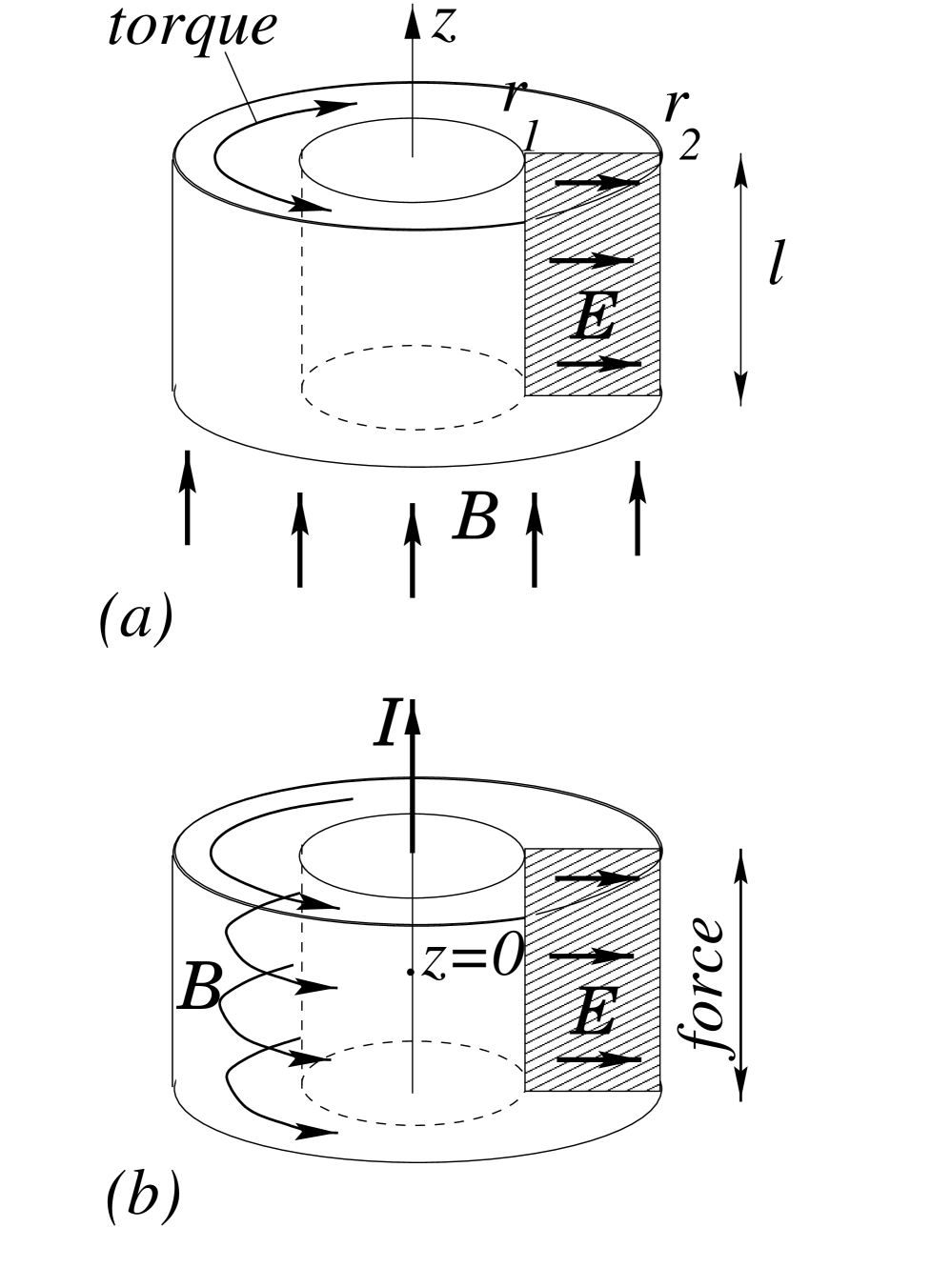
FIG. 1.: (a) Walker & Walker experiment; (b) James’s experiment.

REFERENCES

- [1] H. Minkowski, Nachr. Ges. Wiss. Göttingen (1908) 53.
- [2] M. Abraham, Rend. Circ. Mat. Palermo 28 (1909) 1; M. Abraham, Rend. Circ. Mat. Palermo 30 (1910) 33.
- [3] A. Einstein and J. Laub, Ann. d. Phys. 26 (1908) 541.
- [4] F.N.H. Robinson, Phys. Rept. 16 (1975) 313.
- [5] I. Brevik, Phys. Rept. 52 (1979) 133.
- [6] D.V. Skobeltsyn, Sov. Phys. Uspekhi 16 (1973) 381 [Usp. Fiz. Nauk 110 (1973) 253 (in Russian)]; D.V. Skobeltsyn, Sov. Phys. Uspekhi 20 (1977) 528 [Usp. Fiz. Nauk 122 (1977) 295 (in Russian)].
- [7] V.L. Ginzburg, Sov. Phys. Uspekhi 16 (1973) 434 [Usp. Fiz. Nauk 110 (1973) 309 (in Russian)]; V.L. Ginzburg and V.A. Ugarov, Sov. Phys. Uspekhi 19 (1976) 94 [Usp. Fiz. Nauk 118 (1976) 175 (in Russian)]; V.L. Ginzburg, Sov. Phys. Uspekhi 20 (1977) 546 [Usp. Fiz. Nauk 122 (1977) 325 (in Russian)].
- [8] S. Antoci and L. Mihich, Eur. Phys. J. D3 (1998) 205; S. Antoci and L. Mihich, Nuovo Cim. B112 (1997) 991.
- [9] L.L. Hirst, Rev. Mod. Phys. 69 (1997) 607.
- [10] M. von Laue, Z. Phys. 128 (1950) 387; M. von Laue, in: “Albert Einstein als Philosoph und Naturforscher”, Ed. P.A. Schilpp (W. Kohlhammer Verlag: Stuttgart, 1955) 364; see also F. Beck, Z. Phys. 134 (1953) 136; H.A. Haus, Physica 43 (1969) 77.
- [11] J.P. Gordon, Phys. Rev. A8 (1973) 14.
- [12] G.B. Walker and G. Walker, Can. J. Phys. 55 (1977) 2121; G.B. Walker, D.G. Lahoz, and G. Walker, Can. J. Phys. 53 (1975) 2577; G.B. Walker and D.G. Lahoz, Nature 253 (1975) 339; G.B. Walker and G. Walker, Nature 263 (1976) 401; G.B. Walker and G. Walker, Nature 265 (1977) 324.
- [13] R.P. James, Force on permeable matter in time-varying fields, Ph.D. Thesis (Dept. of Electrical Engineering, Stanford Univ.: 1968); R.P. James, Proc. Nat. Acad. Sci. (USA) 61 (1968) 1149. A detailed description and discussion of James’s experiment can be found in [5], pp. 155-158.
- [14] F.W. Hehl and Yu.N. Obukhov, Foundations of classical electrodynamics (Birkhäuser: Boston, 2003).
- [15] P. Poincelot, C.R. Acad. Sci. Paris, Série B 264 (1967) 1064; P. Poincelot, C.R. Acad. Sci. Paris, Série B 264 (1967) 1179; P. Poincelot, C.R. Acad. Sci. Paris, Série B 264 (1967) 1225; P. Poincelot, C.R. Acad. Sci. Paris, Série B 264 (1967) 1560.