Liquid-vapor oscillations of water in hydrophobic nanopores

Abstract

Water plays a key role in biological membrane transport. In ion channels and water-conducting pores (aquaporins), one dimensional confinement in conjunction with strong surface effects changes the physical behavior of water. In molecular dynamics simulations of water in short (0.8 nm) hydrophobic pores the water density in the pore fluctuates on a nanosecond time scale. In long simulations (460 ns in total) at pore radii ranging from 0.35 nm to 1.0 nm we quantify the kinetics of oscillations between a liquid-filled and a vapor-filled pore. This behavior can be explained as capillary evaporation alternating with capillary condensation, driven by pressure fluctuations in the water outside the pore. The free energy difference between the two states depends linearly on the radius. The free energy landscape shows how a metastable liquid state gradually develops with increasing radius. For radii larger than ca. 0.55 nm it becomes the globally stable state and the vapor state vanishes. One dimensional confinement affects the dynamic behavior of the water molecules and increases the self diffusion by a factor of two to three compared to bulk water. Permeabilities for the narrow pores are of the same order of magnitude as for biological water pores. Water flow is not continuous but occurs in bursts. Our results suggest that simulations aimed at collective phenomena such as hydrophobic effects may require simulation times longer than 50 ns. For water in confined geometries, it is not possible to extrapolate from bulk or short time behavior to longer time scales.

1 Introduction

Channel and transporter proteins control flow of water, ions and other solutes across cell membranes. In recent years several channel and pore structures have been solved at near atomic resolution (1, 2, 3, 4, 6, 5) which together with three decades of physiological data (7) and theoretical and simulation approaches (8) allow us to describe transport of ions, water or other small molecules at a molecular level. Water plays a special role here: it either solvates the inner surfaces of the pore and the permeators (for example, ions and small molecules like glycerol), or it is the permeant species itself as in the aquaporin family of water pores (9, 10, 11) or in the bacterial peptide channel gramicidin A (gA), whose water transport properties are well studied (12, 13, 14). Thus, a better characterization of the behavior of water would improve our understanding of the biological function of a wide range of transporters. The remarkable water transport properties of aquaporins—water is conducted through a long (ca. 2 nm) and narrow (ca. 0.3 nm diameter) pore at bulk diffusion rates while at the same time protons are strongly selected against—are the topic of recent simulation studies (15, 16).

The shape and dimensions of biological pores and the nature of the pore lining atoms are recognized as major determinants of function. How the behavior of water depends on these factors is far from understood (17). Water is not a simple liquid due to its strong hydrogen bond network. When confined to narrow geometries like slits or pores it displays an even more diverse behavior than already shown in its bulk state (18, 19).

A biological channel can be crudely approximated as a “hole” through a membrane. Earlier molecular dynamics (MD) simulations showed pronounced layering effects and a marked decrease in water self diffusion in infinite hydrophobic pore models (20, 21). Recently, water in finite narrow hydrophobic pores was observed to exhibit a distinct two-state behavior. The cavity is either filled with water at approximately bulk density (liquid-like) or it is almost completely empty (vapor-like) (22, 23). Similar behavior was seen in Gibbs ensemble Monte Carlo simulations (GEMC) in spherical (24) and cylindrical pores (25).

In our previous simulations (23) we explored model pores of the dimensions of the gating region of the nicotinic acetylcholine receptor nAChR (26). Hydrophobic pores of radius $R\geq 0.7$ nm were filled during the whole simulation time (up to 6 ns) whereas narrow ones ($R\leq 0.4$ nm) were permanently empty. Changing the pore lining from a hydrophobic surface to a more hydrophilic (polar) one rendered even narrow pores water—and presumably ion—conducting. At intermediate radii ($0.4$ nm $<R<0.7$ nm) the pore-water system was very sensitive to small changes in radius or character of the pore lining. In a biological context, a structure close to the transition radius would confer the highest susceptibility to small conformational rearrangements (i.e. gating) of a channel.

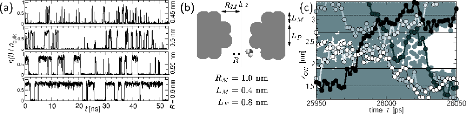
Figure 1: (a) Oscillating water density in model pores of increasing pore radius $R$. The water density $n(t)$ (in units of the bulk water density $n_{\text{bulk}}$) over the simulation time shows strong fluctuations on a greater than ns time scale ($50$ ps moving average smoothing). Two distinctive states are visible: open at approximately $n_{\text{bulk}}$ (liquid water), and closed with very few or no water in the pore (water vapor). (b) The pore model consists of methane pseudo atoms of van der Waals radius $0.195$ nm. A water molecule is drawn to scale. (c) Permeant water molecules in a $R=0.55$ nm pore as it switches from the open to the closed state. $z$-coordinates of the water oxygen atoms are drawn every 2 ps. The mouth and pore region are indicated by horizontal broken and solid lines. Five trajectories are shown explicitly. The white water molecule permeates the pore within 54 ps whereas the black one only requires about 10 ps.

We have extended these simulations to beyond 50 ns in order to explore the longer timescale behavior of the water-pore system. Starting from the observed oscillations in water density (Fig. 1a) we analyze the kinetics and the free energy of the system. We compare the water transport properties of the pores to experimental and theoretical data.

2 Methods

2.1 Model

The pore model was designed to mimic the dimensions of a biological pore [e.g., the gate region of nAChR (26)], whilst retaining the tractability of a simple model. Cylindrical pores of finite length were constructed from concentric rings of pseudo atoms (Fig. 1b). These hydrophobic pseudo atoms have the characteristics of methane molecules, i.e. they are uncharged Lennard-Jones (LJ) spheres with a van der Waals radius of 0.195 nm. The pore consists of two mouth regions (radius $R_{M}=1$ nm, length $L_{M}=0.4$ nm) and an inner pore region ($L_{P}=0.8$ nm) of radius $0.35\ \text{nm}\leq R\leq 1.0\ \text{nm}$, which is the minimum van der Waals radius of the cavity. The centers of the pore lining atoms are placed on circles of radius $R+0.195$ nm. The model was embedded in a membrane mimetic, a slab of pseudo atoms of thickness ca. 1.5 nm or 1.9 nm. Pseudo atoms were harmonically restrained to their initial position with a force constant of $1000$ kJ mol^-1 nm^-2, resulting in positional fluctuations of ca. 0.1 nm, comparable to those of pore lining atoms in membrane protein simulations although this does not allow for global collective motions as in real proteins.

2.2 Simulation Details

MD simulations were performed with gromacs v3.0.5 (27) and the SPC water model (28). The LJ-parameters for the interaction between a methane molecule and the water oxygen are $\epsilon_{\text{CO}}=0.906493$ kJ mol^-1 and $\sigma_{\text{CO}}=0.342692$ nm from the gromacs force field. The integration time step was 2 fs and coordinates were saved every 2 ps. With periodic boundary conditions, long range electrostatic interactions were computed with a particle mesh Ewald method [real space cutoff 1 nm, grid spacing 0.15 nm, 4th order interpolation (29)] while the short ranged van der Waals forces were calculated within a radius of 1 nm. The neighbor list (radius 1 nm) was updated every 10 steps.

Weak coupling algorithms (30) were used to simulate at constant temperature ($T=300$ K, time constant 0.1 ps) and pressure ($P=1$ bar, compressibility $4.5\times 10^{-5}$ bar^-1, time constant 1 ps) with the $x$ and $y$ dimensions of the simulation cell held fixed at 6 nm (or 3.9 nm for the 80 ns simulation of the $R=0.35$ nm pore). The length in $z$ was 4.6 nm in both cases (ensuring bulk-like water behavior far from the membrane mimetic).

The large (small) system contained about 700 (300) methane pseudo atoms and 4000 (1500) SPC water molecules. Simulation times $T_{\text{sim}}$ ranged from 52 ns to 80 ns (altogether 460 ns). Bulk properties of SPC water were obtained from simulations in a cubic cell of length 3 nm (895 molecules) with isotropic pressure coupling at 300 K and 1 bar for 5 ns.

2.3 Analysis

Time courses and density

For the density time courses (Fig. 1a) the pore occupancy $N(t)$, i.e. the number of water molecules within the pore cavity (a cylinder of height $L_{P}=0.8$ nm containing the pore lining atoms) was counted. The density $n(t)$ is given by $N(t)$ divided by the water-accessible pore volume $V=L_{P}\,\pi R_{\text{eff}}^{2}$ and normalized to the bulk density of SPC water at 300 K and 1 bar ($n_{\text{bulk}}=53.67\pm 0.03$ mol l^-1). The effective pore radius for all pores is $R_{\text{eff}}=R-\delta R$. Choosing $\delta R=0.03$ nm fixes the density $\langle N\rangle/V$ in the (most bulk-like) $R=1.0$ nm-pore at the value calculated from the radial density, $R_{0}^{-1}\!\!\int_{0}^{R_{0}}\!\!\!\,n(r)\,dr$, where $R_{0}=1.05$ nm is the radius at which $n(r)$ vanishes.

The density $n(\mathbf{r})$ was determined on a grid of cubic cells with spacing 0.05 nm. Two- and one-dimensional densities were computed by integrating out the appropriate coordinate(s). A probabilistic interpretation of $n(\mathbf{r})$ leads to the definition of the potential of mean force (PMF) of a water molecule $\beta F(\mathbf{r})=-\ln[n(\mathbf{r})/n_{\text{bulk}}]$ with $\beta^{-1}=k_{B}T$, via Boltzmann-sampling of states.

Free energy density and chemical potential

The Helmholtz free energy as a function of the pore occupancy $N$ at constant $T=300$ K for a given pore with volume $V$ was calculated from the probability distribution $p(N)$ of the occupancy as $\beta F(T,V,N)=-\ln p(N)$ and transformed into a free energy density $f(T,n)=F/V$. A fourth order polynomial in $n$ was least-square fitted to $\beta f(T,n)$. The chemical potential $\mu(T,n)=\partial f(T,n)/\partial n$ was calculated as the analytical derivative of the polynomial.

The $\beta f$ curves obtained for different radii $R$ from the simulations are only determined within an unknown additive constant $f_{0}(T;R)$ but a thermodynamic argument shows that all these curves coincide at $n=0$: For $n=0$ no water is in the pore, so the free energy differential is simply $dF=-S\,dT+2\gamma\,dA$ with the constant surface tension of the vacuum (inside the pore)-water (outside) interface of area $A=\pi R^{2}$. At constant $T$ this implies $F(R)=2\gamma\,A+\text{const}(T)$, so that the free energy density $f(T,n=0;R)=F(R)/V=2\gamma\,A/(L\,A)=2\gamma/L$ of a pore with radius $R$ and length $L$ is independent of $R$. Hence, all free energy density curves necessarily coincide at $n=0$ and $f_{0}$ is a function of $T$ only.

Kinetics

The time series $n(t)/n_{\text{bulk}}$ of the water density in the pore was analyzed in the spirit of single channel recordings (31) by detecting open (high-density; in the following denoted by a subscript $o$) and closed (approximately zero density; subscript $c$) pore states, using a Schmitt-trigger with an upper threshold of 0.65 and a lower threshold of 0.15 . A characteristic measure for the behavior of these pores is the openness $\langle\omega\rangle=T_{o}/T_{\text{sim}}$, i.e. the probability for the pore being in the open state (23) with errors estimated from a block-averaging procedure (27). The distribution of the lifetimes $t_{\alpha}$ of state $\alpha=\{o,c\}$ are exponentials $\tau_{\alpha}^{-1}e^{-t_{\alpha}/\tau_{\alpha}}$ (data not shown). The maximum-likelihood estimator for the characteristic times $\tau_{o}$ and $\tau_{c}$ is the mean $\tau_{\alpha}=\langle t_{\alpha}\rangle$.

The free energy difference between closed and open state, $\Delta F=F_{c}-F_{o}$, can be calculated in two ways. Firstly, we obtained it from the equilibrium constant $K=T_{c}/T_{o}=(T_{\text{sim}}-T_{o})/T_{o}=\langle\omega\rangle^{-1}-1$ of the two-state system as $\beta\,\Delta F_{\text{kin}}=-\ln K$. Secondly, $\Delta F$ was determined from $p(N)$ as the ratio between the probability that the pore is in the closed state and the probability for the open state: $\beta\,\Delta F_{\text{eq}}=-\ln P_{c}/P_{o}=-\ln\sum_{N\leq N^{\ddagger}}p(N)/\sum_{N>N^{\ddagger}}p(N)$. The definition of state used here is independent of the kinetic analysis. It only depends on $N^{\ddagger}$, the pore occupancy in the transition state, the state of lowest probability between the two probability maxima that define the closed and open state. The relationship involving $K$ can be inverted to describe the openness in terms of $\Delta F(R)$, $\langle\omega(R)\rangle=\bigl{(}1+\exp[-\beta\,\Delta F(R)]\bigr{)}^{-1}$.

Dynamics

The three components of the self-diffusion coefficient were calculated from the Einstein relations $\bigl{\langle}\bigl{(}x_{i}(t)-x_{i}(t_{0})\bigr{)}^{2}\bigr{\rangle}=2D_{i}\,(t-t_{0})$. The simulation box was stratified perpendicular to the pore axis with the central layer containing the pore. During $T_{\text{sim}}$ the mean square deviation (msd) of water molecules in a given layer was accumulated for 10 ps and after discarding the first 2 ps, a straight line was fit to the msd to obtain $D_{i}$. These diffusion coefficients were averaged in each layer for the final result.

The current density (flux per area) was calculated as $j_{0}=\Phi_{0}/A$ from the equilibrium flux $\Phi_{0}=M/T_{\text{sim}}$ with the total number of permeant water molecules $M$ and the effective pore cross section $A=\pi R_{\text{eff}}^{2}$ for pores or $A=L_{x}L_{y}$ for the bulk case, i.e. a simulation box of water with periodic boundary conditions. Permeant water molecules were defined as those whose pore entrance and exit $z$-coordinate differed. In addition, distributions of permeation times were computed.

3 Results and Discussion

The water density in the pore cavity oscillates between an almost empty (closed) and filled (open) state (Fig. 1a). We refer to the water-filled pore state as open because such a pore environment would favorably solvate an ion and conceivably allow its permeation. Conversely, we assume that a pore that cannot sustain water at liquid densities will present a significant energetic barrier to an ion. As shown in Fig. 1c, water molecules can pass each other and often permeate the pore in opposite directions simultaneously.

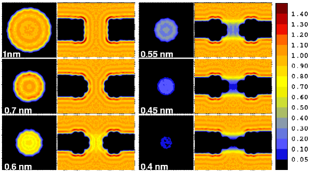
Figure 2: Water density in hydrophobic pores with radii ranging from 1.0 nm to 0.4 nm. Left column in each panel: density $z$-averaged over the length of the pore. Right column: radially averaged density. The density is in units of SPC bulk water at 300 K and 1 bar [plots prepared with xfarbe 2.5 (32)].

Even though the oscillating behavior was already suggested by earlier $1$ ns simulations (23) only at these longer times do clear patterns emerge. The characteristics of the pore-water system change substantially with the pore radius. The oscillations (Fig. 1a) depend strongly on the radius. The water density (Fig. 2) shows large pores to be water-filled and strongly layered at bulk density. With decreasing radius the average density is reduced due to longer closed states even though layer structures remain. The narrowest pores appear almost void of water.

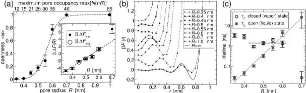
Figure 3: (a) Openness $\langle\omega(R)\rangle$ of hydrophobic pores and free energy difference $\Delta F(R)$ between states (inset). Wide pores are permanently water-filled ($\langle\omega\rangle=1$) whereas narrow ones are predominantly empty ($\langle\omega\rangle\approx 0$). The broken line is the function $\bigl{(}1+\exp[-\beta\,\Delta F_{\text{eq}}(R)]\bigr{)}^{-1}$, with $\Delta F_{\text{eq}}(R)$ determined independently of $\langle\omega(R)\rangle$. $\Delta F(R)$ appears to be a linear function of $R$, regardless if estimated from the kinetics ($\Delta F_{\text{kin}}$) or the equilibrium probability distribution of the pore occupancy ($\Delta F_{\text{eq}}$). (b) Radial potential of mean force of water $F(r)$. Very narrow pores show a relatively featureless PMF, consistent with a predominantly vapor-like state. For larger pore radii, the liquid state dominates. The PMF of the 1 nm pore is very similar to the one of water near a planar hydrophobic slab ($R=\infty$). PMFs are drawn with arbitrary offsets. (c) Kinetics open$\rightleftharpoons$closed. The average lifetime of the open state $\tau_{o}$ depends on the radius exponentially whereas $\tau_{c}$ is approximately constant in the two-state region (cf. Fig. 4) of radii.

The sudden change in behavior is borne out quantitatively by the openness (Fig. 3a), which indicates a sharp increase with increasing radius around $R=0.55$ nm. Although the range of radii over which this transition takes place appears to be small ($0.45$ nm to $0.7$ nm) the cross-sectional area doubles. The maximum number of water molecules actually found in the cavity in our simulations more than doubles from $21$ to $46$ in this range of $R$, so that the average environment which each water molecule experiences changes considerably.

Density

The radial densities in Fig. 2 show destabilisation of the liquid phase with decreasing pore radius. Above $R=0.45$ nm distinctive layering is visible in the pore, and for the larger pores appears as an extension of the planar layering near the slab. For $R<0.45$ nm no such features remain and the density is on average close to $0$. The open state can be identified with liquid water and the closed state with water vapor. In the continuously open 1 nm-pore, the average density $\langle n(t)\rangle/n_{\text{bulk}}$ is $0.82$, but $0.032$ in the closed $0.35$ nm-pore. Brovchenko et al. (33) carried out GEMC simulations of the coexistence of liquid TIP4P water with its vapor in an infinite cylindrical hydrophobic pore of radius $R=1.075$ nm. At $T=300$ K they obtained a liquid density of $0.81$ and a vapor density close to $0$, in agreement with the numbers from our MD simulations.

Analysis of the structure in the radial PMF (Fig. 3b) lends further support to the above interpretation. Water molecules fill the narrow pores ($R\lessapprox 0.45$ nm) homogeneously as it is expected for vapor. For the wider pores, distinct layering is visible as the liquid state dominates. The number of layers increases from two to three, with the central water column being the preferred position initially. As the radius increases, the central minimum shifts toward the wall. For $R=0.7$ nm the center of the pore is clearly disfavored by $0.2\,k_{B}T$. In the largest pore ($R=1.0$ nm), the influence of curvature on the density already seems to be negligible as it is almost identical to the situation near a planar hydrophobic slab.

Kinetics

Condensation (filling of the pore) and evaporation (emptying) occur in an avalanche-like fashion as shown in Fig 1c. In our simulations both events take place within ca. 30 ps, roughly independent of $R$. However, the actual evaporation and condensation processes seem to follow different paths, as we can infer from the analysis of the kinetics of the oscillations. The time series of Fig. 1a reveals that the lifetimes of the open and closed state behave differently with increasing pore radius (Fig. 3c): In the range $0.45\ \text{nm}\leq R\leq 0.6\ \text{nm}$, the average time a pore is in the closed state is almost constant, $\tau_{c}=1.40\pm 0.37$ ns; outside this range no simple functional relationship is apparent. The average open time can be described as an exponential $\tau_{o}(R)=a\exp(R/\zeta)$ with $a=1.3\times 10^{-5}\ \text{ns}$ and $\zeta=4.9\times 10^{-2}\ \text{nm}$ for $0.35\ \text{nm}\leq R\leq 0.7\ \text{nm}$.

$1/\tau_{o}$ is related to the “survival probability” of the liquid state and $1/\tau_{c}$ to that of the vapor state. These times characterize the underlying physical evaporation and condensation processes. Their very different dependence on $R$ implies that these processes must be quite different. The initial condensation process could resemble the evaporation of water molecules from a liquid surface. Evaporating molecules would not interact appreciably, so that this process would be rather insensitive to the area of the liquid-vapor interface $A=\pi R^{2}$ and hence $R$. The disruption of the liquid pore state, on the other hand, displays very strong dependence on the radius. Conceivably, the pore empties once a density fluctuation has created a vapor bubble that can fill the diameter of the pore and expose the wall to vapor, its preferred contact phase. The probability for the formation of a spherical cavity of radius $\lambda$ with exactly $N$ water molecules inside was determined by Hummer et al. (34). From their study we find that the probability $p(\lambda;n)$ for the formation of a bubble of radius $\lambda$ and density below a maximum density $n$ is apparently an exponential. Once a bubble with $\lambda\approx R$ develops, the channel rapidly empties but this occurs with a probability that decreases exponentially with increasing $R$, which corresponds to the observed exponential increase in $\tau_{o}$. In particular, for low density bubbles ($n<0.2\,n_{\text{bulk}}$) we estimate the decay constant in $p(\lambda;n)$ as $2\times 10^{-2}$ nm, which is of the same order of magnitude as $\zeta$.

From the equilibrium constant $K(R)=T_{c}(R)/T_{o}(R)=\exp[-\beta\,\Delta F(R)]$ the free energy difference between the two states $\Delta F=F_{c}-F_{o}$ can be calculated. $\Delta F$ increases linearly with the pore radius (inset of Fig. 3a), $\beta\,\Delta F(R)=a_{0}+a_{1}R$ with $a^{\text{kin}}_{0}=-13.2\pm 1.4$ and $a^{\text{kin}}_{1}=23.7\pm 3.0\ \text{nm}^{-1}$. Together with $K(R)$, the gating behavior of the pore is characterized (31). In this sense, the MD calculations have related the input structure to a “physiological” property of the system. (Note, however, that the time scales of ion channel gating and of the oscillations observed here differ by five orders of magnitude.)

Free energy density

The Helmholtz free energy density $f(T,n;R)$ displays one or two minima (Fig. 4a): one for the empty pore ($n=0$) and one in the vicinity of the bulk density. The 0.45 nm pore is close to a transition point in the free energy landscape: the minimum for the filled pore is very shallow and disappears at smaller radii ($R=0.4$ nm and 0.35 nm). For very large and very small radii, only one thermodynamic stable state exists: liquid or vapor. For intermediate radii, a metastable state appears. Near $R=0.55$ nm both states are almost equally probable although they do not coexist spatially because the pore is finite and small. In infinite pores spatially alternating domains of equal length would be expected (35) and were actually observed in MD simulations (36). The oscillating states in short pores, on the other hand, alternate temporally, thus displaying a kind of “time-averaged” coexistence.

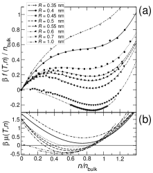
Figure 4: (a) Free energy density $f(T,n)$ at constant $T=300$ K. (b) Chemical potential $\mu(T,n)$. $n$ is the water density in the pore, normalized to $n_{\text{bulk}}=53.7$ mol l^-1. $f$ is given in units of $k_{B}T$ and the inverse of the liquid molecular volume of bulk water ($v_{l}^{-1}=n_{\text{bulk}}$). Two minima correspond to the observed two-state behavior. The vapor state becomes metastable with increasing radius and for $R>0.55$ nm the liquid state is globally stable. $f(T,n;R=1.0\ \text{nm})$ is drawn with an arbitrary offset.

For higher densities $n/n_{\text{bulk}}>1$ the curves start to resemble parabolas, similar to a parabolic $f(T,n)$ seen for cylindrical volumes (data not shown) and spherical cavities (34) in bulk water.

The chemical potential (Fig. 4b) shows the transition from the stable vapor state, $\mu(T,n)>0$, through the two-state regime to the stable liquid state, $\mu(T,n)<0$. The features of $\mu(T,n)$ indicate that the condensation (and evaporation) processes occur in an avalanche-like fashion: Let the density in the pore be at the transition state, the left zero of $\mu$. If the density is perturbed to increase slightly then $\mu$ becomes negative. Every additional molecule added to the pore decreases the free energy further by an amount $\mu$ while the increase in density lowers the chemical potential even more. This leads to the avalanche of condensation. It only stops when the stable state, the right zero of $\mu$, is reached. Now a further addition of molecules to the pore would actually increase the free energy and drive the system back into the stable state. Similarly, a perturbation that decreases the density in the transition state leads to accelerated evaporation.

From the probability distribution $p(N)$ the free energy difference between closed and open state $\Delta F(R)$ is calculated, $a^{\text{eq}}_{0}=-14.9\pm 2.2$ and $a^{\text{eq}}_{1}=26.3\pm 4.1\ \text{nm}^{-1}$, consistent with the estimate from the kinetics. $\Delta F(R)$ (inset of Fig. 3a) shows the transfer of stability from the vapor state for small $R$ to the liquid state for large $R$. The coexistence regime is at $\Delta F(R_{c}=0.57\ \text{nm})=0$.

Dynamics

MD simulations not only allow us to investigate the thermodynamic properties of the system but also the dynamical behavior of individual molecules. A few selected water molecules are depicted in Fig. 1c shortly before the pore empties. They show a diverse range of behaviors and no single-file like motion of molecules is visible in the liquid state. On evaporation (and condensation) the state changes within ca. 30 ps.

Table 1: Dynamical properties of water in hydrophobic pores. $R$ is the van der Waals pore radius, with $R=\infty$ denoting the bulk. $\langle\omega\rangle$ is the openness. The mean permeation time $\langle\tau_{p}\rangle$ is measured relative to the bulk value, $\langle\tau_{p,\text{bulk}}\rangle=29.9\pm 0.1$ ps. The equilibrium current density $j_{0}$ is the total number of permeant water molecules per unit time and unit area ($j_{0,\text{bulk}}=320\pm 3~{}$ns${}^{-1}\,\text{nm}^{-2}$). The diffusion coefficient along the pore axis $D_{z}$ is normalized to the bulk value of SPC water at 300 K and 1 bar ($D_{\text{bulk}}=4.34\pm 0.01\ \text{nm}^{2}\,\text{ns}^{-1}$). One standard deviation errors in the last decimals are given in parentheses.

$R/\text{nm}$		$\langle\omega\rangle$		$\langle\tau_{p}\rangle/\langle\tau_{p,\text{bulk}}\rangle$		$j_{0}/j_{0,\text{bulk}}$		$D_{z}/D_{\text{bulk}}$
0.	35	0.	008(2)	0.	482(61)	0.	025(2)
0.	4	0.	015(5)	0.	421(25)	0.	027(2)	2.	87(9)
0.	45	0.	101(30)	0.	629(12)	0.	109(3)	2.	27(4)
0.	5	0.	181(41)	0.	729(10)	0.	194(4)	1.	91(3)
0.	55	0.	291(89)	0.	786(8)	0.	279(4)	1.	87(3)
0.	6	0.	775(79)	0.	833(5)	0.	721(6)	1.	32(1)
0.	7	0.	999(1)	0.	799(3)	1.	004(7)	1.	25(0)
1.	0	1.	000(0)	0.	819(2)	1.	011(5)	1.	18(0)
$\infty$				1.	000(3)	1.	000(8)	1.	00(0)

The mean permeation time $\langle\tau_{p}\rangle$ in Table 1 increases with the pore radius, i.e. water molecules permeate narrow hydrophobic pores faster than they diffuse the corresponding distance in bulk water (the reference value). This is consistent with higher diffusion coefficients $D_{z}$ in the narrow pores (up to almost three times the bulk value). The diffusion coefficient perpendicular to the pore axis, $D_{xy}$, drops to approximately half the bulk value. Martí and Gordillo (37) also observe increased diffusion in simulations on water in carbon nanotubes ($D_{z}\leq 1.65\,D_{\text{bulk}}$) and a corresponding decrease in $D_{xy}$. Experimental studies on water transport through desformyl gA (13) can be interpreted in terms of a $D_{z}$ of five times the bulk value. Histograms (data not shown) for $\tau_{p}$ show that there is a considerable population of ‘fast’ water molecules (e.g. the black and the dark gray one in Fig. 1c) with $\tau_{p}$ between 2 and 10 ps, which is not seen in bulk water. The acceleration of water molecules in the pore can be understood as an effect of 1D confinement. The random 3D motion is directed along the pore axis and the particle advances in this direction preferentially. The effect increases with decreasing radius, i.e. increasing confinement. The average equilibrium current density $j_{0}$ follows the trend of the openness closely but more detailed time-resolved analysis shows water translocation to occur in bursts in all pores. In narrow pores, bursts occurring during the “closed” state contribute up to 77% of the total flux (data not shown). For single-file pores, simulations (22, 14) and theory (38) also point towards concerted motions as the predominant form of transport.

Capillary condensation

The behavior as described so far bears the hallmarks of capillary condensation and evaporation (39, 40, 19) although it is most often associated with physical systems which are macroscopically extended in at least one dimension such as slits or long pores. Capillary condensation can be discussed in terms of the Kelvin equation (18),

$$\ln\frac{p}{p_{0}}=-\frac{\beta\gamma_{lv}v_{l}}{r},$$ (1)

which describes how vapor at pressure $p$ relative to its bulk-saturated pressure $p_{0}$ coexists in equilibrium with its liquid. Liquid and vapor are divided by an interfacial meniscus of curvature $1/r$ ($r>0$ if the surface is convex); $\gamma_{lv}$ is the surface tension between liquid and vapor and $v_{l}$ the molecular volume of the liquid. Although the Kelvin equation is not expected to be quantitative in systems of dimensions of only a few molecular diameters it is still useful for obtaining a qualitative picture. Curvature $1/r$ and contact angle $\theta$ in a cylindrical pore of radius $R$ are related by $R=r\cos\theta$. With Young’s equation, $\gamma_{wv}=\gamma_{wl}+\gamma_{lv}\cos\theta$, Eq. 1 becomes

$$\ln\frac{p(R)}{p_{0}}=-\frac{\beta(\gamma_{wv}-\gamma_{wl})v_{l}}{R},$$ (2)

independent of the interface. For our system, the surface tension between liquid water and the wall, $\gamma_{wl}>0$, and between vapor and the wall, $\gamma_{wv}>0$, are fixed quantities. The hydrophobicity of the wall implies $\gamma_{wv}<\gamma_{wl}$, i.e. the wall is preferentially in contact with vapor; $v_{l}$ can be considered constant. Hence, for a given pore of radius $R$ there exists one vapor pressure $p(R)>p_{0}$ at which vapor and liquid can exist in equilibrium. Water only condenses in the pore if the actual vapor pressure exceeds $p(R)$. Otherwise, only vapor will exist in the pore. The effect is strongest for very narrow pores. Hence a higher pressure is required to overcome the surface contributions, which stabilize the vapor phase in narrow pores. The pressure fluctuates locally in the liquid bulk “reservoir.” These fluctuations can provide an increase in pressure above the saturation pressure in the pore and thus drive oscillations between vapor and liquid.

Comparison with experiments, simulations, and a theoretical model

Experiments on aquaporins (9, 10) and gA (12, 13) yield osmotic permeability coefficients of water, $p_{f}$, of the order of $10^{-12}$ to $10^{-14}\ \text{cm}^{3}\text{s}^{-1}$. We calculate $p_{f}=\frac{1}{2}\Phi_{0}v_{l}$ from the equilibrium flux of our MD simulations (14) and find that narrow ($R=0.35$ nm and $0.4$ nm), predominantly “closed” pores have $p_{f}\approx 5\times 10^{-14}\ \text{cm}^{3}\text{s}^{-1}$, that is, the same magnitude as Aqp1, AqpZ, and gA (see Table 2).

Table 2: Osmotic permeability coefficient $p_{f}$ and equilibrium flux $\Phi_{0}$ of water in selected simulations and experiments. We used the relationship $p_{f}=\frac{1}{2}\Phi_{0}v_{l}$ from Ref. 14 in order to compare non-equilibrium experiments (upper half of the table) with equilibrium molecular dynamics simulations (lower half). $v_{l}=3.09\times 10^{-23}$ cm³ is the volume of a water molecule in the liquid state.

	Ref.	$p_{f}\times 10^{14}$		$\Phi_{0}$
		[$\text{cm}^{3}\text{s}^{-1}$]		[$\text{ns}^{-1}$]
Aqp1	(9)	4	.9	3	.2
Aqp4	(9)	15		9	.7
AqpZ	(10)	2	.0	1	.3
gA	(12)	1	.6	1	.0
desformyl gA	(13)	110		71
$R=0.35$ nm		4	.0	2	.6
$R=0.40$ nm		5	.7	3	.7
$R=0.45$ nm		30	.0	19	.4
$R=0.50$ nm		66	.5	43	.0
$R=0.55$ nm		117		75	.8
$R=0.60$ nm		363		235
$R=0.70$ nm		700		453
$R=1.0$ nm		1480		956
carbon nanotube	(22)	26	.2	16	.9
desformyl gA (DH)	(14)	10		5	.8

As these pores are longer (ca. $2$ nm) and narrower ($R<0.2$ nm) than our model pores, strategically placed hydrophilic groups (15) seem to be needed to stabilize the liquid state and facilitate water transport in these cases.

Recently Giaya and Thompson (41) presented an analytical mean-field model for water in infinite cylindrical hydrophobic micropores. They predict the existence of a critical radius $R_{c}$ for the transition from a thermodynamically stable water vapor phase to a liquid phase. The crucial parameter that $R_{c}$ depends on is the water-wall interaction. We choose the effective fluid-wall interaction $\epsilon_{\text{eff}}=\rho_{w}\,\epsilon_{fw}$, the product of the density of wall atoms with the well-depth of the fluid-wall interaction potential, as a parameter to compare different simulations because this seems to be the major component in the analytical fluid-wall interaction.

Table 3: Comparison of different studies of water in hydrophobic pores. The wall-atom density $\rho_{w}$ is in units of nm^-3, the fluid-wall interaction $\epsilon_{fw}$ in kJ mol^-1 and the effective interaction strength $\epsilon_{\text{eff}}$ in kJ mol^-1 nm^-3. The critical pore radius $R_{c}$ is given in nm. The pore length was 0.8 nm in this work, 1.7 nm in the carbon nanotube simulations (22) and infinite in the mean field model (41).

Ref.	$\rho_{w}$	$\epsilon_{fw}$		$\epsilon_{\text{eff}}$	$R_{c}$
this work	8	0.	906493	7	$\approx 0.57$
(22)	50	0.	478689	24	$<0.24$
		0.	272937	14	$>0.24$
(41)	110	0		0	1500
		1.	4	154	190
		1.	45	160	0.35
		2.	0	220	0

As shown in Table 3, compared to carbon nanotube simulations our pore has a very small $\epsilon_{\text{eff}}$ and thus can be considered extremely hydrophobic. This explains why Hummer et al. (22) observe permanently water filled nanotubes with a radius of only 0.24 nm although their bare fluid-wall interaction potential is weaker than in our model. The much higher density of wall atoms in the nanotube, however, more than mitigates this. Once they lower their $\epsilon_{\text{eff}}$ to double of our value, they also observe strong evaporation. This suggests that the close packing of wall atoms within a nanotube may result in behavior not seen in biological pores. The mean field model agrees qualitatively with the simulations as it also shows a sharp transition and high sensitivity to $\epsilon_{\text{eff}}$.

4 Conclusions

We have described oscillations between vapor and liquid states in short ($L_{P}=0.8$ nm), hydrophobic pores of varying radius ($0.35$ nm$\leq R\leq 1.0$ nm). Qualitatively, this behavior is explained as capillary evaporation, driven by pressure/density fluctuations in the water “reservoir” outside the pore. Similar behavior is found in simulations by different authors with different water models [SPC (this work), SPC/E, TIP3P (data not shown), TIP3P (22), TIP4P (25)] in different nanopores [atomistic flexible models (this work), carbon nanotubes (22), spherical cavities (24) and smooth cylinders (25, 42)].

We presented a radically simplified model for a nanopore that is perhaps more hydrophobic than in real proteins [although we note the existence of a hydrophobic pore in the MscS channel (6)]. From comparison with experimental data on permeability we conclude that strategically placed hydrophilic groups are essential for the functioning of protein pores. The comparatively high permeability of our “closed” pores suggests pulsed water transport as one possible mechanism in biological water pores. Local hydrophobic environments in pores may promote pulsatory collective transport and hence rapid water and solute translocation.

Our results indicate new, intrinsically collective dynamic behavior not seen on simulation time scales currently considered sufficient in biophysical simulations. These phase oscillations in simple pores—a manifestation of the hydrophobic effect—require more than 50 ns of trajectory data to yield a coherent picture over a free energy range of $6\,k_{B}T$. We thus cannot safely assume that the behavior of water within complex biological pores may be determined by extrapolation from our knowledge of the bulk state or short simulations alone.

Acknowledgments

This work was funded by The Wellcome Trust. Our thanks to all of our colleagues for their interest in this work, especially Joanne Bright, José Faraldo-Gómez, Andrew Horsfield and Richard Law.

References

- Doyle et al. (1998) Doyle, D. A., Morais-Cabral, J., Pfützner, R. A., Kuo, A., Gulbis, J. M., Cohen, S. L., Chait, B. T., & MacKinnon, R. (1998) Science 280, 69–77.
- Chang et al. (1998) Chang, G., Spencer, R. H., Lee, A. T., Barclay, M. T., & Rees, D. C. (1998) Science 282, 2220–2226.
- Fu et al. (2000) Fu, D., Libson, A., Miercke, L. J., Weitzman, C., Nollert, P., Krucinski, J., & Stroud, R. M. (2000) Science 290, 481–486.
- Sui et al. (2001) Sui, H., Han, B. G., Lee, J. K., Walian, P., & Jap, B. K. (2001) Nature 414, 872–878.
- Dutzler et al. (2002) Dutzler, R., Campbell, E. B., Cadene, M., Chait, B. T., & MacKinnon, R. (2002) Nature 415, 287–294.
- Bass et al. (2002) Bass, R. B., Strop, P., Barclay, M., & Rees, D. C. (2002) Science 298, 1582–1587.
- Hille (2001) Hille, B. (2001) Ion Channels of Excitable Membranes (Sinauer Associates, Sunderland MA, U.S.A.), 3rd ed.
- Tieleman et al. (2001) Tieleman, D. P., Biggin, P. C., Smith, G. R., & Sansom, M. S. P. (2001) Quart. Rev. Biophys. 34, 473–561.
- Yang et al. (1997) Yang, B., van Hoek, A. N., & Verkman, A. S. (1997) Biochemistry 36, 7625–7632.
- Pohl et al. (2001) Pohl, P., Saparov, S. M., Borgnia, M. J., & Agre, P. (2001) Proc. Natl. Acad. Sci. USA 98, 9624–9629.
- Fujiyoshi et al. (2002) Fujiyoshi, Y., Mitsuoka, K., de Groot, B. L., Philippsen, A., Grubmüller, H., Agre, P., & Engel, A. (2002) Curr. Opin. Struct. Biol. 12, 509–515.
- Pohl and Saparov (2000) Pohl, P. & Saparov, S. M. (2000) Biophys. J. 78, 2426–2434.
- Saparov et al. (2000) Saparov, S. M., Antonenko, Y. N., , & Pohl, P. (2000) Biophys. J. 79, 2526–2534.
- de Groot et al. (2002) de Groot, B. L., Tieleman, D. P., Pohl, P., & Grubmüller, H. (2002) Biophys. J. 82, 2934–42.
- Tajkhorshid et al. (2002) Tajkhorshid, E., Nollert, P., Jensen, M. Ø., Miercke, L. J., O’Connell, J., Stroud, R. M., & Schulten, K. (2002) Science 296, 525–530.
- de Groot and Grubmüller (2001) de Groot, B. L. & Grubmüller, H. (2001) Science 294, 2353–2357.
- Finkelstein (1987) Finkelstein, A. (1987) Water Movement Through Lipid Bilayers, Pores, and Plasma Membranes. Theory and Reality (John Wiley & Sons, New York).
- Christenson (2001) Christenson, H. K. (2001) J. Phys.: Condens. Matter 13, R95–R133.
- Gelb et al. (1999) Gelb, L. D., Gubbins, K. E., Radhakrishnan, R., & Sliwinska-Bartkowiak, M. (1999) Rep. Prog. Phys. 62, 1573–1659.
- Lynden-Bell and Rasaiah (1996) Lynden-Bell, R. M. & Rasaiah, J. C. (1996) J. Chem. Phys. 105, 9266–9280.
- Allen et al. (1999) Allen, T. W., Kuyucak, S., & Chung, S.-H. (1999) J. Chem. Phys. 111, 7985–7999.
- Hummer et al. (2001) Hummer, G., Rasaiah, J. C., & Noworyta, J. P. (2001) Nature 414, 188–190.
- Beckstein et al. (2001) Beckstein, O., Biggin, P. C., & Sansom, M. S. P. (2001) J. Phys. Chem. B 105, 12902–12905.
- Brovchenko et al. (2000) Brovchenko, I., Paschek, D., & Geiger, A. (2000) J. Chem. Phys. 113, 5026–5036.
- Brovchenko and Geiger (2002) Brovchenko, I. & Geiger, A. (2002) J. Mol. Liquids 96–97, 195–206.
- Unwin (2000) Unwin, N. (2000) Phil. Trans. Roy. Soc. London B 355, 1813–1829.
- Lindahl et al. (2001) Lindahl, E., Hess, B., & van der Spoel, D. (2001) J. Mol. Mod. 7, 306–317. http://www.gromacs.org.
- Hermans et al. (1984) Hermans, J., Berendsen, H. J. C., van Gunsteren, W. F., & Postma, J. P. M. (1984) Biopolymers 23, 1513–1518.
- Darden et al. (1993) Darden, T., York, D., & Pedersen, L. (1993) J. Chem. Phys. 98, 10089–10092.
- Berendsen et al. (1984) Berendsen, H. J. C., Postma, J. P. M., DiNola, A., & Haak, J. R. (1984) J. Chem. Phys. 81, 3684–3690.
- Sakmann and Neher (1983) Sakmann, B. & Neher, E., eds. (1983) Single-Channel Recordings (Plenum Press, New York).
- Preusser (1989) Preusser, A. (1989) ACM Trans. Math. Softw. 15, 79–89. http://www.fhi-berlin.mpg.de/grz/pub/xfarbe/.
- Brovchenko et al. (2001) Brovchenko, I., Geiger, A., & Oleinikova, A. (2001) Phys. Chem. Chem. Phys. 3, 1567–1569.
- Hummer et al. (1996) Hummer, G., Garde, S., García, A. E., Pohorille, A., & Pratt, L. R. (1996) Proc. Natl. Acad. Sci. USA 93, 8951–8955.
- Privman and Fisher (1983) Privman, V. & Fisher, M. E. (1983) J. Stat. Phys. 33, 385–417.
- Peterson et al. (1988) Peterson, B. K., Gubbins, K. E., Heffelfinger, G. S., Marconi, U. M. B., & van Smol, F. (1988) J. Chem. Phys. 88, 6487–6500.
- Martí and Gordillo (2001) Martí, J. & Gordillo, M. C. (2001) Phys. Rev. E 64, 021504–1.
- Berezhkovskii and Hummer (2002) Berezhkovskii, A. & Hummer, G. (2002) Phys. Rev. Lett. 89, 065403–1–4.
- Rowlinson and Widom (1982) Rowlinson, J. S. & Widom, B. (1982) Molecular Theory of Capillarity (Clarendon Press, Oxford).
- Evans (1990) Evans, R. (1990) J. Phys.: Condens. Matter 2, 8989–9007.
- Giaya and Thompson (2002) Giaya, A. & Thompson, R. W. (2002) J. Chem. Phys. 117, 3464–3475.
- Allen et al. (2002) Allen, R., Melchionna, S., & Hansen, J.-P. (2002) Phys. Rev. Lett. 89, 175502–1–175502–4.