The power law character of off-site power failures

A. John Arul ¹¹1Corresponding author’s e-mail: arul@igcar.ernet.in, C. Senthil Kumar^♮, S. Marimuthu and Om Pal Singh Reactor Physics Division, Indira Gandhi Centre for Atomic Research,^♮AERB-Safety Research Institute
Kalpakkam, 603 102, India

Abstract

A study on the behavior of off-site AC power failure recovery times at three nuclear plant sites is presented. It is shown, that power law is appropriate for the representation of failure frequency-duration correlation function of off-site power failure events, based on simple assumptions about component failure and repair rates. It is also found that the annual maxima of power failure duration follow Frechet distribution, which is a type II asymptotic distribution, strengthening our assumption of power law for the parent distribution. The extreme value distributions obtained are used for extrapolation beyond the region of observation.

off-site power, power law, extreme value

1. Introduction
Estimation of off-site power failure characteristics is important for the safe design and operation of nuclear power plants. The emergency power supply requirements are based on the ability to forecast the maximum credible loss of off-site power (LOSP) duration during the life time of the plant. The observed data is available only over a period of less than two decades and scarce on long duration failures. We address two questions: first, what is the nature of the parent distribution, i.e., the form of frequency-duration correlation function and second how to extrapolate for failure durations longer than the observed maximum.

First we show, based on simple assumptions about the off-site power supply system component failure and repair rates, that the frequency-duration correlation function is a power law of the form, $y\propto x^{-k}$ . Next, it is established that the distribution of annual maxima, of observed failures follow Type II asymptotic distribution (Frechet distribution, see Johnson 1970). This result strengthens the premise, that the parent distribution for power failure duration-correlation is power law in character. Extreme value analysis is also used to make extrapolations for more number of years than observed, for instance to estimate the most probable loss of off-site power duration in say, 50 or 100 years.

2. Off-site power failure frequency-duration function
The off-site AC power at a plant may be lost due to supply failure from the power grid or because of plant centered equipment failure like station transformer, feeders, breakers etc. The grid failure could be a minor grid disturbance or grid collapse. The grid power may also fail due to severe environmental conditions. Baranowsky, (1988) has used Weibull functions of the form $(\lambda_{i}e^{(-\alpha_{i}t^{\beta})})$ for representing the frequency of off-site power failure events of each type, exceeding a given duration. Although the fits are good, it would be better if some physical basis could be established for the fitted function. Further considering the scarcity of data, instead of a series of stretched exponentials a single function would be preferable. It is postulated here that there is a mixture of power failure rates $\lambda_{i}$ with a certain probability density $g(\lambda_{i})$ as $\lambda_{i}\in\{\lambda_{i}|i=1..N\}$ . Similarly for the repair rates $\mu_{i}\in\{\mu_{i}|i=1..N\}$ . That is, there are different kinds of equipment each with a specific $\lambda_{i}$ and $\mu_{i}$ . Then the probability of observing a failure of duration $t^{\prime}\geq t$ is

P(t^{\prime}\geq t)=\sum_{i}{g(\lambda_{i})\exp(-\mu_{i}t)}d

(1)

where $e^{(-\mu_{i}t)}$ is the probability that the failed component is not restored in time t, assuming constant repair rate $\mu_{i}$ . Since more frequent failures are generally repairable in shorter times compared to rare failures which take more time to set right, it is assumed that $\mu\propto\lambda$ , with this assumption in equation 1, and going over to the continuous limit we get,

P(t^{\prime}\geq t)=\int{g(\lambda)e^{(-c\lambda t)}d\lambda}

(2)

Where $c>0$ is a constant of proportionality. The form of $g$ is not known, however it is known (Johnson, 1970) that if gamma distribution

g(\lambda)=\alpha e^{(-\alpha\lambda)}(\alpha\lambda)^{(k-1)}/\Gamma(k)

for constants $\alpha,k>0$ , is assumed for $g$ , then Pareto distribution is obtained as the cumulative distribution function $F(t)=1-P(t^{\prime}\geq t)$ . That is the solution of equation 2 is

P(t^{\prime}\geq t)={1\over(1+{c\over\alpha}t)^{k}}

(3)

For large $t$ , $P(t)$ goes like $P(t)\backsim(\theta/t)^{k};k>0;\theta>0;t\geq 0$ , where $\theta=\alpha/c$ and

F(t)\approx 1-(\theta/t)^{k}

(4)

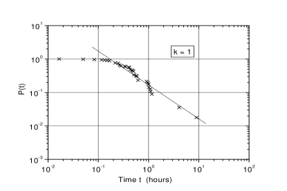
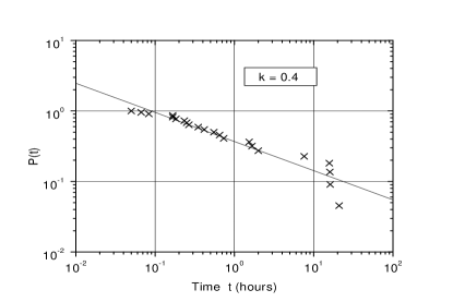
This family includes Cauchy, $t$ and $F$ distributions. The function P(t) is plotted for data observed at two plant sites, over a period of 15-20 years, in Fig. 1 and 2. The plots show P(t) versus LOSP time $t$ in Log-Log scale. The linear fits are shown alongside, which confirm the power law character of the distribution. In Fig. 1 there is considerable deviation from straight line for the first few points. This is due to the fact that for small values of $t$ , i.e., for ${c\over\alpha}t<<1$ , P(t) is virtually constant, and the power law dependence manifests fully for large $t$ . The LOSP frequency-duration correlation function has the same time dependence as it will be different from $P(t)$ only by a constant factor.

3. Extreme value analysis of LOSP duration
The distribution of maximum of $m$ observations of the random variable $t$ , distributed as F(t) is,

\lim_{m\longrightarrow\infty}F(t)^{m}=G(t)

The non-trivial limit distribution G(t) is obtained by appropriate scaling of the variable $t$ ,

\lim_{m\longrightarrow\infty}F((t-b_{m})/\theta_{m})^{m}=G(t)

when $F(t)$ is of the form of equation 4, the asymptotic limit, with $b_{m}=0$ is

G(t)=e^{-(\theta/t)^{k}}

(5)

which is one of the three possible asymptotic limits, that is, a type II extreme value distribution (Fisher et al., 1928 and Gumbel, 1954) also known as Frechet distribution. For finite $m$ equation 5 is written as $G_{m}(t)=e^{-(\theta_{m}/t)^{k}}$ .

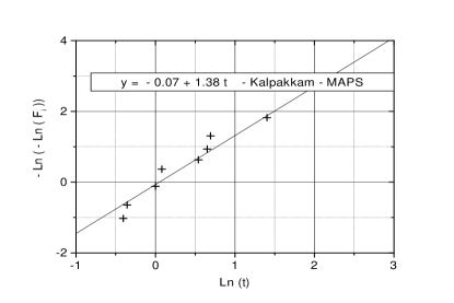
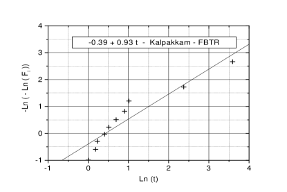
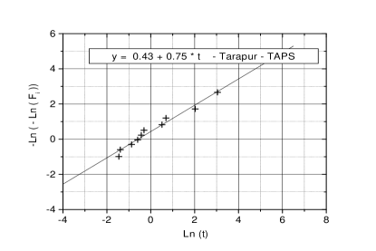
Extreme value analysis of LOSP data collected in (Theivarajan 1999, Marimuthu et al., 2000 and Kumar et al., 2002), is done as follows. The annual maximum $t_{i}$ for each location is arranged in ascending order as, $t_{1}<t_{2}<...<t_{N}$ . The plotting points F(i) are calculated as

F(i)=(i-0.3)/(N+0.4)

(See Karl Bury, 1999), where N is the number of years over which the data is collected. The $F(i)$ approximate the median of the distribution free estimate of the cumulative distribution function. When $-ln(-ln(F(i)))$ are plotted against $ln(t)$ , where $t$ is the power failure duration, straight lines are obtained as depicted in Figs. 3, 4 and 5, as expected from equation 5. The exponents $k$ obtained from the slope, is shown in the respective figures.

The distribution of maximum in any $n$ years will be

G_{n}(t)=G_{m}(t)^{n}=e^{-(\theta_{n}/t)^{k}}

(6)

where

\theta_{n}=\theta_{m}n^{(1/k)}

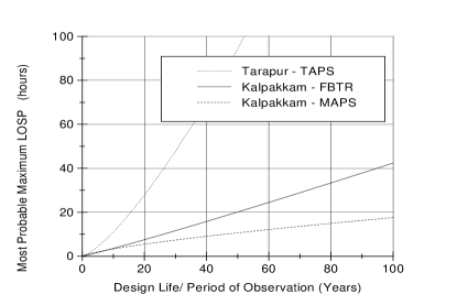
The most probable maximum in $n$ years of observation, obtained from equation 6 is,

\widehat{t}=\theta({nk\over{k+1}})^{(1/k)}

The most probable maximum $\widehat{t}$ is plotted in Fig. 6, for the three locations. The relatively higher value of most probable maximum for TAPS and FBTR cases is due to higher incidence of recorded on-site power distribution equipment failure. From Fig. 6 we can infer that, for instance a 20 h LOSP extrema is likely in TAPS site in 15 y, whereas events of such duration are expected to occur only in 50 years and 100 years respectively for the FBTR and MAPS sites. These conclusions are based on the data collected from these sites and results are indicative only.

4. Conclusion
The nature of the relationship of off-site power failure duration and its frequency is studied and it is found to have power law dependence. Plausible physical basis for the observed behavior is given. The power law nature of asymptotic behavior is confirmed by performing an extreme value analysis of the data. The extreme value distribution is also used to extrapolate beyond observed LOSP durations.

It is interesting to note that, power laws have been observed in a variety of natural and man made settings like, frequency distribution of words (Zipf, 1949), distribution of incomes, earthquake magnitudes and recently in internet topology (Faloutsos et al., 1999), to name a few. Based on the intimate connection between power laws and the ideas of self organized criticality (Bak et al., 1987), it can be said that off-site power distribution system seems to evolve into a critical state, where failures of longer duration are not infrequent, as one would expect for exponential distribution. Although it is convenient not to consider cutoffs to failure duration from a theoretical perspective, it would be better if methods could be devised to include cutoffs considering the finiteness of the system.

References

1.

Bak P., Tang C., and Wiesenfeld K. 1988. Self-Organized Criticality, Phys. Rev. A, 38, 364.
2.

Baranowski, P. W. 1988. Evaluation of Station Blackout Accidents at Nuclear Power Plants, NUREG-1032, USNRC, Washington.
3.

Faloutsos M., Faloutsos P., and Faloutsos C. 1999. On Power-Law Relationships of the Internet Topology, SIGCOMM ’99, pp. 251-262.
4.

Fisher R. A. and Tippet L.H.C., 1928, Limiting forms of the frequency distributions of the largest or smallest members of a sample, Proceedings of the Cambridge Philosophical Society 24, pp. 180-190.
5.

Gumbel, E. J. 1954. Statistical Theory of Extreme Values and Some Practical Applications, National Bureau of Standards Applied Mathematics Series 33, Washington.
6.

Johnson N. L. and Kotz S. 1970. Distributions in statistics continuous univariate distributions-1, John Wiley & Sons, New York.
7.

Karl Bury, 1999. Statistical Distributions in Engineering, Cambridge University Press.
8.

Kumar, C. S., Arul, A. J., Anandapadmanaban, B., Marimuthu, S. 2002. Estimation of Station Blackout Frequency in FBTR, ROMG/FBTR/S-AX-01/52000/SAR-38.
9.

Marimuthu, S., Theivarajan, N., Kumar, C. S., and John Arul, A. 2000. Statistics of Loss of Off-Site Power at Kalpakkam, Rev. A., PFBR/01160/DN/1000, Kalpakkam, India.
10.

Theivarajan, N. 1999. Recommended Design Basis Data for the Loss of Off-site Power, IGCAR Internal Report, PFBR/51100/DN/1001, Kalpakkam, India.
11.

Zipf, G. K. 1949. Human Behavior and Principle of Least Effort: An Introduction to Human Ecology, Addison Wesley, Cambridge, Massachusetts.

Refer to caption — Figure 1: P(t) versus loss of off-site power duration $t$ for site Kalpakkam-MAPS