Present address: ]LPGP, Bât. 210, UPS, F-91405 Orsay

Dynamical analysis of the nonlinear growth of the $m=n=1$ resistive internal mode

Abstract

A dynamical analysis is presented that self-consistently takes into account the motion of the critical layer, in which the magnetic field reconnects, to describe how the $m=n=1$ resistive internal kink mode develops in the nonlinear regime. The amplitude threshold marking the onset of strong nonlinearities due to a balance between convective and mode coupling terms is identified. We predict quantitatively the early nonlinear growth rate of the $m=n=1$ mode below this threshold.

The large scale dynamics and confinement properties of tokamak plasmas depend intimately on the behavior of $m=n=1$ magnetohydrodynamic (MHD) internal kink modes. This has motivated an intense, long-lasting, experimental and theoretical research, notably devoted to study their implication in magnetic reconnection or as triggers of the sawtooth oscillations and crashes. These phenomena typically proceed beyond the linear regime, that is now rather well understood but assumes very small amplitudes of the modes. To offer a quantitative, predictive description of their nonlinear manifestations remains a difficult objective of both academic interest and very practical importance. This is especially relevant for the design of fusion burn experiments in which the fulfilment of linear stability constraints is challenged by the search for ignition. Such devices are thus expected to operate at best close to marginal stability for the $m=n=1$ ideal mode so that nonlinear effects come into play for fairly small values of the mode amplitude Coppi02 ; Odblom02 .

In this Letter, we focus on the $m=n=1$ resistive mode Coppi76 in which a finite resistivity $\eta$ destabilizes the otherwise marginally stable ideal MHD internal kink mode. Since Kadomtsev’s scenario Kadomtsev predicting the complete reconnection of the helical flux within the $q=1$ surface on a timescale of order $\eta^{-1/2}$, that later appeared too large to account for observations, the nonlinear behavior of the $m=n=1$ mode has become a somewhat controversial issue. Some numerical simulations suggested that the mode still grows exponentially into the nonlinear regime waddell which was supported by a theoretical model Hazeltine86 . Later some analytic studies Waelbroeck89 , supported by numerical simulations Biskamp91 , rather predicted a transition to an algebraic growth early in the nonlinear stage. This result was challenged by Aydemir’s recent simulations using a dynamical mesh Aydemir97 . These did show the linear exponential stage evolving towards an algebraic stage, yet this was brutally interrupted by a second nonlinear exponential growth. A modified Sweet-Parker model was able to fit continuously both stages of evolution Aydemir97 and the transition related to a change in the geometry of the current sheet Wang99 . However, some fundamental questions remain unanswered or unclear. Among them, how to relate the transition threshold with $\eta$ ? or what is the role of the $q$-profile ? The aim of this Letter is to describe analytically how the $m=n=1$ resistive mode develops in the nonlinear regime, by focusing on the equations controlling plasma dynamics.

We consider the low-$\beta$ reduced MHD equations

$$\frac{\partial U}{\partial t} = \left[\phi,U\right]+\left[J,\psi\right]$$ (1)

$$\frac{\partial\psi}{\partial t} = \left[\phi,\psi\right]+\eta(J-J_{0})$$ (2)

assuming helical symmetry FirpoMIT . Only a single angular variable is then involved in the problem, namely the helical angle $\alpha\equiv\varphi-\theta$, with $\varphi$ the toroidal and $\theta$ the poloidal angles. $U=\nabla_{\bot}^{2}\phi$ is the vorticity and $J=\nabla_{\bot}^{2}\psi$ the helical current density, with $\nabla_{\bot}^{2}\equiv r^{-1}\partial_{r}r\partial_{r}+r^{-2}\partial_{\alpha}^{2}$. Time is normalized by the poloidal Alfvén time ($t\rightarrow t/\tau_{Hp}$), the radial variable by the minor radius ($r\rightarrow r/a$) and $\eta$ is the dimensionless resistivity, inverse of the magnetic Reynolds number $S$ ($\eta\equiv S^{-1}=\tau_{Hp}/\tau_{R}$) with the poloidal Alfvén time $\tau_{Hp}=\left(\mu_{0}\rho_{0}\right)^{1/2}R/B_{0\varphi}$ and resistive time $\tau_{R}=\mu_{0}a^{2}/\eta_{0}$. The Poisson brackets are defined by $\left[\phi,U\right]=-\mathbf{\hat{\varphi}}\cdot\left(\mathbf{\nabla}_{\bot}\phi\times\mathbf{\nabla}_{\bot}U\right)=r^{-1}\left(\partial_{r}\phi\partial_{\alpha}U-\partial_{r}U\partial_{\alpha}\phi\right)$. $\phi$ and $\psi$ are the plasma velocity and helical magnetic field potentials expressed in cylindrical coordinates, so that the velocity is $\mathbf{v}=\mathbf{\hat{\varphi}}\times\mathbf{\nabla}_{\bot}\phi$ and the magnetic field is $\mathbf{B}=B_{0\varphi}\mathbf{\hat{\varphi}}+\mathbf{\hat{\varphi}}\times\mathbf{\nabla}_{\bot}\left(\psi-r^{2}/2\right)$.

We consider MHD equilibria given by $\phi_{0}=0$ and by an helical magnetic flux $\psi_{0}\left(r\right)$, related to the safety profile $q(r)$ through $d_{r}\psi_{0}=r\left[1-1/q(r)\right]$, such that $q=1$ for an internal radius $r=r_{s0}$. Thus $d_{r}\psi_{0}\left(r_{s0}\right)=0$. This means that the low-frequency ideal linear equations associated to (1)-(2) are singular at $r=r_{s0}$, with a formally diverging current density. This marks the presence of a critical layer in which the dynamics differs considerably from the outer one and where resistivity enters to cure the singularity.

We wish to analyse perturbatively the time evolution of the $m=1$ mode. For this, we assume that only the $m=1$ mode is destabilized initially with an amplitude $A_{0}$, neglect all ideal MHD transients and restrict to the linear resistive timescale $\tau\equiv\eta^{1/3}t$. We do not consider the somehow ill-posed, singular limit $\eta\rightarrow 0$, but instead realize that two small parameters are indeed competing in this problem, namely the small given resistivity $\eta$ and the time-dependent amplitude $A(\tau)$ of the linear $m=1$ mode. This introduces some subtleties in the amplitude expansion. The order one solution is given by linear theory using an asymptotic analysis Coppi76 to match inner and outer solutions. Excitation of the $m=1$ mode leads to a self-consistent correction to the location of the critical layer. One estimates the amplitude threshold, scaling with $\eta$, at which next order solution is required and the procedure iterated. Separability in time and space propagates at each order resulting in an amplitude expansion in $A$. As in any perturbative approach, the solution is formally known when the order one solution is. This is given by the linear theory reviewed now.

Let $f_{n}^{(m)}$ be the projection on $\exp(im\alpha)$ of any function $f$ at order $n$. In the inner resistive layer, Eqs. (1)-(2) read

$$\left[\frac{\partial}{\partial\tau}\frac{\partial^{2}}{\partial x^{2}}\phi_{1}^{(1)}+i\kappa_{0}x\frac{\partial^{2}}{\partial x^{2}}\psi_{1}^{(1)}\right]w^{-1} = 0$$ (3)

$$\left[\frac{\partial}{\partial\tau}\psi_{1}^{(1)}+i\kappa_{0}x\phi_{1}^{(1)}-\frac{\partial^{2}}{\partial x^{2}}\psi_{1}^{(1)}\right]w = 0$$ (4)

where we define $\kappa_{0}\equiv\psi_{0}^{\prime\prime}\left(r_{s0}\right)/r_{s0}$. In these equations, $x$ is the stretched coordinate $x=\left(r-r_{s0}\right)/w$ and $w\equiv\eta^{1/3}$ the magnitude of the width of the critical layer giving the maximal resistive ordering Coppi76 in (3)-(4). In the layer, radial derivatives are large, since $\partial_{r}=w^{-1}\partial_{x}$ and (3)-(4) are the dominant equations for $w\ll 1$. There is one unstable solution, the $m=1$ resistive mode, with growth rate $\hat{\gamma}_{L}=\kappa_{0}^{2/3}=q^{\prime}(r_{s0})^{2/3}$. Real space potentials read

$$\psi_{1}\left(x,\alpha,\tau\right) = A_{0}\exp\left(\hat{\gamma}_{L}\tau\right)g_{L}\left(\frac{\kappa_{0}^{1/3}x}{\sqrt{2}}\right)\cos\alpha$$ (5)

$$\phi_{1}\left(x,\alpha,\tau\right) = -\frac{A_{0}}{\sqrt{2}}\exp\left(\hat{\gamma}_{L}\tau\right)g_{L}^{\prime}\left(\frac{\kappa_{0}^{1/3}x}{\sqrt{2}}\right)\sin\alpha$$ (6)

where $g_{L}$ is the function

$$g_{L}\left(s\right)=\frac{s}{2}\mathop{\mathrm{erfc}}\left(s\right)-\frac{1}{2\sqrt{\pi}}\exp(-s^{2}).$$ (7)

This solution was chosen to satisfy the matching asymptotic conditions $g_{L}^{\prime}\left(-\infty\right)=1$ and $g_{L}^{\prime}\left(+\infty\right)=0$. This analysis has to be complemented with the derivation of the outer solution. On the resistive timescale, this amounts to solve, at leading (zero) order in $w$, a linear system of ideal MHD equilibria, singular at $r=r_{s0}$ FirpoMIT . This illustrates the passive character of the outer domain. We only retain here that, given the asymptotic and boundary conditions imposing $\psi_{1}^{\prime(1)}(r_{s0}^{+})=0$ and $\psi_{1}^{(1)}(1)=0$, the outer linear $m=1$ solution $\psi_{1}^{(1)}(r)$ is identically vanishing for $r_{s0}<r\leq 1$.

Linear theory breaks down when, in the resistive critical layer, nonlinear terms due to mode couplings, e.g. in Eq. (1) $\left[\phi_{1},U_{1}\right]\sim w^{-3}A^{2}$, balance linear ones, i.e. $\kappa_{0}xw\partial_{\alpha}J_{1}\sim A/w$ in Eq. (3). Thus $A(\tau)=\mathcal{O}(\eta^{2/3})$ marks the onset of second order terms. Before pursuing the analysis on the critical layer, we need to track it and self-consistently estimate its location. The total magnetic flux in the critical layer is now $\psi\left(x,\alpha,\tau\right)=\eta^{2/3}\psi_{0}^{\prime\prime}\left(r_{s0}\right)x^{2}/2+\psi_{1}\left(x,\alpha,\tau\right)$. To follow continuously the linear stage, we define the ’backbone’ $r_{s}\left(\alpha,\tau\right)$ of the critical layer as the ’neutral’ field line with $\partial_{r}\psi\left(r_{s}\right)\equiv 0$. Writing $r_{s1}\left(\alpha,\tau\right)=r_{s}\left(\alpha,\tau\right)-r_{s0}=wx_{1}(\alpha,\tau)$ with $\partial_{x}\psi(x_{1})=0$, this gives

$$r_{s1}\left(\alpha,\tau\right)\simeq-\frac{A\left(\tau\right)}{\eta^{1/3}}\frac{\kappa_{0}^{1/3}g_{L}^{\prime}\left(0\right)}{\sqrt{2}\psi_{0}^{\prime\prime}\left(r_{s0}\right)}\cos\alpha$$ (8)

which relates to the shift of the core plasma inside the $q=1$ surface due to the kink instability. Then the x-point shift $r_{s1}\left(\alpha=\pi,\tau\right)$ goes like $A(\tau)/\eta^{1/3}$, consistently with Aydemir’s numerical results Aydemir97 . Thus the critical radius starts to leave the linear critical layer band, centered on $r_{s0}$, when $r_{s1}\left(\alpha,\tau\right)$ becomes of the order $\eta^{1/3}$ for some $\alpha$, that is when $A\left(\tau\right)\gtrsim\eta^{2/3}$. This is again the threshold marking the end of the linear stage. We need now to define a generalized stretched coordinate in the critical layer as $x=\left(r-r_{s}\left(\alpha,\tau\right)\right)/w$. The replacements $\partial_{\tau}\rightarrow\partial_{\tau}-w^{-1}\left(\partial r_{s}/\partial\tau\right)\partial_{x}$ and $\partial_{\alpha}\rightarrow\partial_{\alpha}-w^{-1}\left(\partial r_{s}/\partial\alpha\right)\partial_{x}$ are then required note1 .

The second order critical layer equations involve an inhomogeneous part composed of quadratic terms in the order one solutions (5), (6) and (8). This acts to force the growth of the $m=0$ and $m=2$ perturbations but brings no contribution to the $m=1$ dynamics. Therefore the $m=1$ equations (3)-(4) are unchanged, except that, due to the motion of the critical layer (8), one needs to replace $\kappa_{0}$ in (3)-(4) by the time-dependent average

$$\kappa^{(0)}(\tau)\equiv\frac{1}{2\pi}\int\limits_{0}^{2\pi}\frac{\partial_{r}^{2}\psi\left[r_{s}\left(\alpha,\tau\right)\right]}{r_{s}\left(\alpha,\tau\right)}d\alpha.$$ (9)

This introduces a generalized linear system of equations. Neglecting the initially zero amplitudes of the $m=0$ and $m=2$ perturbations in front of $A(\tau)$, the second order correction to the location of the critical layer is given by $r_{s2}\left(\alpha,\tau\right)\simeq-\left(2\psi_{0}^{\prime\prime}\left(r_{s0}\right)\right)^{-1}\psi_{0}^{\prime\prime\prime}\left(r_{s0}\right)r_{s1}\left(\alpha,\tau\right)^{2}$. The validity threshold of the second order solution is reached when the instantaneous critical line moves out of the critical layer of width $w$ centered on $r_{s0}+r_{s1}\left(\alpha,\tau\right)$ for some $\alpha$. This corresponds to $r_{s2}\left(\alpha,\tau\right)\sim w$, that is to $r_{s1}\left(\alpha,\tau\right)^{2}\sim\eta^{1/3}$, which gives $A(\tau)=\mathcal{O}\left(\eta^{1/2}\right)$. This threshold in the amplitude of the linear $m=1$ mode marks the onset of third order terms, that will contribute again to the $m=1$ dynamics. Its brutal manifestation is visible on Aydemir’s plots Aydemir97 . They clearly report a transition in the $m=1$ kinetic energy when this becomes of order $\eta/2$ note2 , namely around $5\times 10^{-8}$ for $\eta=10^{-7}$ and around $5\times 10^{-6}$ for $\eta=10^{-5}$.

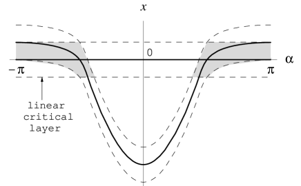
Figure 1: Picture in the $(x,\alpha)$ space of the initial linear critical layer and of a nonlinear one centered on the instantaneous transverse neutral field line (in bold). The grey region represents their overlapping domain within which the gradients of linear potentials are $\mathcal{O}(w^{-1})$-large.

At third order, cubic terms in the order one solutions or quadratic terms coupling the $m=0$ and $m=2$ second order terms to the $m=1$ first order ones appear in the inhomogeneous part of the critical layer equations and modify the $m=1$ dynamics. These terms involve some radial derivatives, e.g. $\partial_{r}\phi_{1}^{(1)}$, that are $\mathcal{O}(w^{-1})$-large only within the linear layer. Locality enters here the analysis since the dominant contribution of these mode coupling terms comes from the localized zone in $(r,\alpha)$ where the instantaneous and linear critical layers overlap. This is depicted by the grey shaded region in Fig. 1. The novelty is that, in this region, mode couplings are now able to balance convective derivatives, both being dominant with respect to linear terms. More explicitly, while, e.g. in the Eq. (1) written in the region where the instantaneous and linear critical layers overlap, the magnitude of linear terms is $\partial_{\tau}\partial_{r}^{2}\phi^{(1)}\sim w^{-2}A(\tau)$, convective terms are of the order of $\partial_{\tau}r_{s2}^{(0)}\partial_{r}^{3}\phi_{1}^{(1)}\sim w^{-5}A^{3}$. Thus linear terms become negligible for $A(\tau)\gg\eta^{1/2}$, which marks the onset of the fully nonlinear regime for the $m=1$ mode. Moreover, convective terms, e.g. $\partial_{\tau}r_{s2}^{(0)}\partial_{r}^{3}\phi_{1}^{(1)}\sim w^{-5}A^{2}\partial_{\tau}A$, equilibrate mode coupling terms, such as $-r_{s0}^{-1}\partial_{r}\phi_{1}^{(-1)}\partial_{\alpha}r_{s1}^{(1)}\partial_{r}U_{1}^{(1)}\sim w^{-5}A^{3}$ coming from $\left[\phi,U\right]$ in the shear-Alfvén law (1). The nonlinear growth rate derives from this balance. As $\kappa^{(0)}(\tau)$ is no longer involved in those convective and mode coupling terms, there is no extra time-dependence in the dominant equations, so that the nonlinear growth rate is just equal, by continuity, to the growth rate of the $m=1$ mode when $A(\tau)$ becomes of order $\eta^{1/2}$. Its value depends notably on the equilibrium $q$-profile as we shall see below. After some spatial averaging, a rough summary of the time evolution of the $m=1$ mode amplitude may be then finally written as

$$\frac{dA}{dt}-\gamma\left(t\right)A+\frac{c}{\eta}A^{2}\left(\frac{dA}{dt}-\gamma\left(t_{NL}\right)A\right)=0,$$ (10)

where the initial value of the growth rate $\gamma\left(0\right)$ is $\gamma_{L}$ and where the early time dependence of $\gamma$ comes from the motion of the critical layer and is computed quantitatively below. In Eq. (10), $c$ is a constant of order one and $t_{NL}$ denotes the (magnitude of the) time at which $A$ becomes of order $\eta^{1/2}$. Eq. (10) describes effectively the transition between two (almost) exponential stages. Because $\phi_{3}^{(1)}$and $\psi_{3}^{(1)}$ are zero at the onset of the third order regime, Eq. (10) remains valid during some stage even if the structure and scaling of the critical layer should substantially change as the generalized linear stage is left.

For the convective exponential stage to be fully valid, the overlap between the linear and instantaneous critical layers should be large enough. One expects then a qualitatively different late behavior of the $m=1$ dynamics if the x-point region is far away from the linear layer when $A(\tau)=\mathcal{O}\left(\eta^{1/2}\right)$, that is, due to (8), if $\eta^{-1/6}\ggg 1$. This regime is extremely challenging to reach numerically but may be satisfied in tokamak plasmas.

We finally examine the early nonlinear effects on the growth rate of the $m=1$ mode due to the motion of the critical layer. This amounts to solve the system of differential equations (3)-(4) for $\kappa_{0}$ replaced with $\kappa^{(0)}\left(\tau\right)$, defined in (9). It can be checked that, as long as the order of magnitude of $A\left(\tau\right)$ is lower than $\eta^{1/2}$, $\kappa^{(0)}\left(\tau\right)$ may be approximated by $\left(2\pi\right)^{-1}\int\nolimits_{0}^{2\pi}r_{s}\left(\alpha,\tau\right)^{-1}\psi_{0}^{\prime\prime}\left[r_{s}\left(\alpha,\tau\right)\right]d\alpha$ at leading order. This expression will be retained in the numerical computations. The time-dependent growth rate is defined as $\hat{\gamma}\left(\tau\right)\equiv d_{\tau}A/A.$ In this generalized linear system, there is one condition shared with the linear derivation: for a solution in separate variables $\tau$ and $x$, it is that $\hat{\gamma}\left(\tau\right)/\kappa\left(\tau\right)$ be constant. This constant is then fixed by continuity with the linear solution at time zero giving

$$\frac{\hat{\gamma}\left(\tau\right)}{\kappa^{(0)}\left(\tau\right)}=\frac{\hat{\gamma}_{L}}{\kappa_{0}}=\kappa_{0}^{-1/3}.$$ (11)

Here one implicitly assumes that the spatial part of the linear eigenfunctions remains valid note3 . The instantaneous critical radius is $r_{s}\left(\alpha,\tau\right)=r_{s0}+\eta^{1/3}x_{s}\left(\alpha,\tau\right)$ where $x_{s}(\alpha,\tau)$ is given by the approximate expression

$$x_{s}\left(\alpha,\tau\right)=H^{-1}\left(-\frac{A(\tau)\kappa_{0}^{1/3}\cos\alpha}{\eta^{2/3}\sqrt{2}\psi_{0}^{\prime\prime}(r_{s0})}\right).$$ (12)

$H^{-1}$ denotes the inverse of the monotonously growing function defined by $H(x)\equiv x/g_{L}^{\prime}\left(\kappa_{0}^{1/3}x/\sqrt{2}\right)$. Due to the asymmetric nature of the $m=1$ resistive eigenfunctions (7), $H^{-1}(x)$ is very asymmetric, grossly equal to $x$ below $x=0$ and exponentially small above. This confers a much more important weight on negative arguments of $H^{-1}$ than on positive ones in the averaging (9). The magnetic island has thus a higher effective contribution to the early nonlinear correction of the growth rate than the region of x-point. A rough estimate of the angular average of $x_{s}$ is given by $x_{s}^{(0)}(\tau)\simeq-\left(2\pi\right)^{-1}A\left(\tau\right)\kappa_{0}^{1/3}/\left(\eta^{2/3}\sqrt{2}\psi_{0}^{\prime\prime}(r_{s0})\right)\int\nolimits_{-\pi/2}^{\pi/2}d\alpha\cos\alpha$. Eq. (11) defines a first order differential equation in $A(\tau)$ that admits then the approximate form $\hat{\gamma}\left(\tau\right)\simeq\hat{\gamma}_{L}+\eta^{1/3}d_{r}\left[r^{-1}\psi_{0}^{\prime\prime}(r)\right]\left(r_{s0}\right)x_{s}^{(0)}(\tau)$. Going back to time $t$ and to $\gamma_{L}\equiv\eta^{1/3}\hat{\gamma}_{L}$, this gives

$$\frac{dA}{dt}\simeq\gamma_{L}A(t)-C_{0}A(t)^{2}$$ (13)

where $C_{0}=$ $\left(q_{0}^{\prime}+r_{s0}q_{0}^{\prime\prime}-2r_{s0}q_{0}^{\prime 2}\right)/\left(\pi\sqrt{2}r_{s0}^{2}q_{0}^{\prime 2/3}\right)$ and the index $0$ denotes an evaluation at $r_{s0}$. Eq. (13) shows the first nonlinear contribution to the $m=1$ evolution. The early behavior of the $m=1$ growth rate is thus $\gamma(t)\simeq\gamma_{L}-C_{0}A_{0}\exp\left(\gamma_{L}t\right)$. In order to check numerically these analytic predictions for the generalized linear stage, that brings the first nonlinear contributions to the growth rate, we used Aydemir’s initial conditions Aydemir97 . The safety profile is $q(r)=q_{m}\left\{1+r^{4}\left[\left(q_{a}/q_{m}\right)^{2}-1\right]\right\}^{1/2}$ with $q_{m}=0.9$, $q_{a}=3$, giving $C_{0}>0$. The differential equation (11) was integrated numerically for $A_{0}=\sqrt{2}\times 10^{-5.5}$ corresponding to an initial kinetic energy in the $m=1$ mode of the order $10^{-11}$.

Figure 2: Analytic nonlinear growth rate corresponding to the initial conditions used in Ref. Aydemir97 and resistivity $\eta=10^{-7}$, neglecting third order convective effects coming into play when $A(t)$ becomes of order $\eta^{1/2}$. This occurs for $t\simeq 1000$.

The nonlinear growth rate $\gamma\left(t\right)\equiv\eta^{1/3}\hat{\gamma}(\tau)$ is plotted on Fig. 2 for $S=10^{7}$. This curve appears to be in fine agreement with the Figure 1 of Ref. Aydemir97 for times $t$ roughly below 1000 Alfvèn times.

Fig. 3 illustrates the influence of the $q$-profile around $r_{s0}$ on the time evolution of $\gamma$ due to (9). A sudden bump in the nonlinear growth could thus even be observed, before the onset of convective effects, for the special shape of $q$ chosen in Fig. 3. Moreover, some $q$-profile may induce a saturation of $A$ below the convective threshold and lead to partial reconnection. Most importantly, the approach described here may be transposed to model the early nonlinear behavior of a variety of internal kinks such as two-fluid Aydemir92 ; Rogers96 ; Biskamp97 and/or collisionless Cafaro98 models.

Figure 3: Analytic nonlinear growth rate for the same initial values as in Fig. 2 but with a modified equilibrium safety profile $q(r)$. Its behavior around $r_{s0}$ is plotted in the insert.

Discussions with L. Sugiyama are gratefully acknowledged. MCF thanks A. Aydemir for several communications on his simulations. This work was supported in part by the U.S. Department of Energy.

References

• (1) B. Coppi et al., FT/P2-10, 19th IAEA Fusion Energy Conference, Lyon (2002).
• (2) A. Oedblom et al., Phys. Plasmas 9, 155 (2002).
• (3) B. Coppi, R. GalvΓ£o, M. N. Rosenbluth, and P. H. Rutherford, Sov. J. Plasma Phys. 2, 3276 (1976); G. Ara et al., Ann. Physics 112, 443 (1978).
• (4) B.B. Kadomtsev, Fiz. Plasmy 1, 710 (1975) [Sov. J. Plasma Phys. 1, 389 (1975)].
• (5) B.V. Waddell, M.N. Rosenbluth, D.A. Monticello, and R.B. White, Nucl. Fusion 16, 3 (1976).
• (6) R.D. Hazeltine, J.D. Meiss, and P.J. Morrison, Phys. Fluids 29, 1633 (1986).
• (7) F.L. Waelbroeck, Phys. Fluids B 1, 2372 (1989).
• (8) D. Biskamp, Phys. Fluids B 3, 3353 (1991).
• (9) A.Y. Aydemir, Phys. Rev. Lett. 78, 4406 (1997).
• (10) X. Wang and A. Bhattacharjee, Phys. Plasmas 6, 1674 (1999).
• (11) M.-C. Firpo, to be published.
• (12) It can be checked that angular contributions in Laplacians are negligible in the critical layer for $A(\tau)\ll\eta^{1/3}$.
• (13) The factor $1/2$ in the kinetic energy of the $m=1$ mode comes from the expression of the linear solution $\phi_{1}$ in (6).
• (14) This is partly justified by the matching to the vanishing order one outer solution for rβ‰₯rs​0π‘Ÿsubscriptπ‘Ÿπ‘ 0r\geq r_{s0}.
• (15) A.Y. Aydemir, Phys. Fluids B 4, 3469 (1992).
• (16) B. Rogers and L. Zakharov, Phys. Plasmas 3, 2411 (1996).
• (17) D. Biskamp and T. Sato, Phys. Plasmas 4, 1326 (1997).
• (18) E. Cafaro et al., Phys. Rev. Lett. 80, 4430 (1998).