Distance, dissimilarity index, and network community structure

Abstract

We address the question of finding the community structure of a complex network. In an earlier effort [H. Zhou, Phys. Rev. E (2003)], the concept of network random walking is introduced and a distance measure defined. Here we calculate, based on this distance measure, the dissimilarity index between nearest-neighboring vertices of a network and design an algorithm to partition these vertices into communities that are hierarchically organized. Each community is characterized by an upper and a lower dissimilarity threshold. The algorithm is applied to several artificial and real-world networks, and excellent results are obtained. In the case of artificially generated random modular networks, this method outperforms the algorithm based on the concept of edge betweenness centrality. For yeast’s protein-protein interaction network, we are able to identify many clusters that have well defined biological functions.

I Introduction

A graph (network) of vertices (nodes) and edges is a useful tool in describing the interactions between different agents of a complex system. For example if we want to analyze protein-protein physical interactions in yeast Saccharomyces cerevisiae Uetz et al. (2000), we would like to denote each protein as a distinct vertex of a graph, and setup an edge between two vertices if the corresponding proteins have direct physical interactions. Many such kinds of networks are constructed in sociological, biological, and technological fields, and they usually have very complicated connection patterns. What one needs is a method that is capable of classifying vertices of a complex network into different clusters (communities). If a network is appropriately decomposed into a series of functional units, (a) the structure of the network can be better understood and the relationship between its different components will be clear, (b) the principal function of each cluster can be inferred from the functions of its members, and (c) possible functions for members of a cluster can be suggested by comparing the functions of other members. Network clustering techniques are therefore very important in the emerging fields of bioinformatics and proteomics.

A good clustering method needs to satisfy two conditions: First, the inherent structure of the network should be reserved; Second, it should provide a quantified resolution parameter to mark the significance of the clusters obtained at each level of the partitioning process. The global organization of a network should already be identified at low resolutions and more and more fine structures emerge as the resolving power is increased.

Many existing methods Wasserman and Faust (1994); Ravasz et al. (2002) only take account of local information of each vertex, such as number of nearest-neighbors shared with other vertices, number of vertex-independent paths to other vertices, etc.. Recently, Girvan and Newman Girvan and Newman (2002) suggested an elegant global algorithm which extended the concept of vertex betweenness centrality of Freeman Freeman (1977) also to edges. Their algorithm works iteratively by removing the current edge(s) of the highest degree of betweenness centrality. When applying to an ensemble of random modular networks, this algorithm greatly outperforms some conventional methods Girvan and Newman (2002). On the other hand, it does not provide a parameter to quantify the differences between communities.

In reference zho (a) a Brownian particle is $``$introduced” into a network to $``$measure” the distances between vertices. In the present work, we extend the basic idea of zho (a) by defining, based on this distance matrix, a quantity called the dissimilarity index between nearest-neighboring vertices. The dissimilarity index signifies to what extent two nearest-neighboring vertices would like to be in the same community. A hierarchical algorithm is then worked out; it takes use of information on the dissimilarity indices and decompose a network into a hierarchical sequence of clusters. Each of the communities is characterized by an upper and a lower dissimilarity threshold.

The method, which could work on unweighted as well as weighted networks, is applied to several artificial and real networks, and very satisfying results are obtained. For the case of random modular networks, the present algorithm outperforms the method of Girvan and Newman Girvan and Newman (2002). When applying the algorithm to the protein-protein interaction network of yeast, we are able to identify many protein clusters which have well defined biological functions.

In section II we review the distance measure of reference zho (a) and define a dissimilarity index for each pair of nearest-neighboring vertices. A dissimilarity-index-based hierarchical algorithm is outlined in section III, and applied to two kinds of artificially generated networks and four real-world networks in section IV. We conclude our work in section V.

II Distance measure and dissimilarity index

In the opinion of Flake, Lawrence, and Giles Flake et al. (2000), a community in a (sub)graph should satisfy the requirement that each vertex’s total intra-community interaction be stronger than the total interaction with other vertices in the (sub)graph. This turns out to be a very strong constraint. In this work, we weaken this condition and require only that a vertex should have stronger total interaction with other vertices of its own community than with vertices of any another community of the (sub)graph.

We consider a connected network of $N$ vertices and $M$ edges. The network’s connection pattern is specified by the generalized adjacency matrix $A$. We assume that the value of each non-zero element of matrix $A$ (say $A_{ij}$) denotes the interaction strength between vertex $i$ and $j$. The distance, $d_{ij}$, from vertex $i$ to vertex $j$ is defined as the average number of steps needed for a Brownian particle on this network to move from vertex $i$ to vertex $j$ zho (a). At each vertex (say $k$) the Brownian particle will jump in the next step to a nearest-neighboring vertex (say $l$) with probability $P_{kl}=A_{kl}/\sum_{m=1}^{N}A_{km}$. The distance matrix thus defined is asymmetric (in general $d_{ij}\neq d_{ji}$), and it is calculated by solving $N$ linear-algebraic equations zho (a).

Taking any vertex $i$ as the origin of the network, then the set $\{d_{i1},\cdots,d_{i,i-1},d_{i,i+1},\cdots,d_{iN}\}$ measures how far all the other vertices are located from the origin. Therefore it is actually a perspective of the whole network with vertex $i$ being the viewpoint. Suppose vertex $i$ and $j$ are nearest-neighbors ($A_{ij}>0$), the difference in their perspectives about the network can be quantitatively measured. We define the dissimilarity index, $\Lambda(i,j)$, by the following expression:

$$\Lambda(i,j)={\sqrt{\sum\limits_{k\neq i,j}^{N}[d_{ik}-d_{jk}]^{2}}\over(N-2)}.$$ (1)

If two nearest-neighboring vertices $i$ and $j$ belong to the same community, then the average distance $d_{ik}$ from $i$ to any another vertex $k$ ($k\neq i,j$) will be quite similar to the average distance $d_{jk}$ from $j$ to $k$, therefore the network’s two perspectives (based on $i$ and $j$, respectively) will be quite similar. Consequently, $\Lambda(i,j)$ will be small if $i$ and $j$ belong to the same community and large if they belong to different communities.

III the algorithm

We exploit the dissimilarity index to decipher the community structure of a network. After the distance matrix $\{d_{ij}\}$ and the dissimilarity indices for all the nearest-neighboring vertices $\{\Lambda(i,j)\}$ are obtained, the algorithm works as follows:

1.

Intially the whole network is just one single community. This community is assigned an upper dissimilarity threshold $\theta_{\rm upp}$ equalling to the maximum value of all the different dissimilarity indices.

2.

For each community, a resolution threshold parameter $\theta$ is introduced and is assigned the initial value $\theta_{\rm upp}$ of that community. The algorithm is unable to discriminate between two nearest-neighboring vertices $i$ and $j$ when $\Lambda(i,j)\leq\theta$; if this happens, vertices $i$ and $j$ are marked as $``$friends”.

3.

The $\theta$ value is decreased differentially. All edges in the community are examined to see whether two nearest-neighboring vertices are friends. Different friends sets of the community are then formed, each of which contains all the friends of the vertices in the set. There may also be vertices in the community that do not have any friends. Each of these vertices is moved to the friends set that has the strongest interaction with it. After this operation, vertices of the community are distributed into a number of disjointed sets (this number may be unity).

4.

Each vertex in a subcluster should have stronger interaction with vertices within this subcluster than with vertices of any another subcluster of this community. To fulfill this requirement, we perform a local adjustment process: move each of the vertices that fail to meet this requirement to the friends set that has the strongest total interaction with it. This adjustment process is performed simultaneously for all these unstable vertices and is repeated until no unstable vertices remains.

5.

If vertices of the community remain together, the algorithm returns to step 3. If they are divided into two or more sets, then the community under processing is assigned a lower dissimilarity threshold $\theta_{\rm low}$ equalling to the current $\theta$ value, and it is no longer considered. Each of the identified subsets of this community is regarded as a new (lower-level) community, with upper dissimilarity threshold $\theta_{\rm upp}$ equalling to the current $\theta$ value. The algorithm returns to step 2 to work with another identified community.

6.

After all the (sub)communities are processed, a dendrogram is drawn to demonstrate the relationship between different communities as well as the upper and lower dissimilarity thresholds of each community. The vertex set of each community is also reported.

The above procedure could be easily implemented with C++ programming language. The source code as well as the data for the examples studied in the following section will be made publicly available zho (b).

IV Applications

We test the performance of the above-mentioned algorithm by applying it first to two kinds of artificial networks and to three real-world networks.

IV.1 Artificial random modular networks

To quantitatively compare with the work of Girvan and Newman Girvan and Newman (2002) the algorithm is first applied to a random modular network. The network has $128$ nodes, which are divided into $4$ modules of size $32$ each. Each vertex has on average $16$ edges connecting to other vertices, and on average $\overline{z}_{\rm out}$ of each vertex’s edges are to vertices of other modules. All the edges are setup randomly with these two fixed expectation values. The present method is able to recover the modular structure of the network up to $\overline{z}_{\rm out}\simeq 7$. It slight outperforms the method of Girvan and Newman Girvan and Newman (2002) in performance. For example, working on an ensemble of random graphs with $\overline{z}_{\rm out}=6.0$ by the present method, on average only $4.5$ vertices are misclassified, each of which is assigned a cluster identity different from those of the majority of vertices of its module; while on average about $13$ vertices are misclassified by the method of Girvan and Newman Girvan and Newman (2002).

Figure 1: The community structure of a random modular network of $128$ vertices and $1067$ unweighted edges (see the main text for the rules how such a network is generated). Here and in following figures, in the pattern $xx$-$yy$, the number $yy$ after the hyphen denotes the group-identity of vertex $xx$ according to information from other sources.

In figure 1, the community structure of a randomly generated modular network with $\overline{z}_{\rm out}=6.0$ is demonstrated. When the resolution threshold is beyond $0.323$, the network as a whole could be regarded as a giant community. At resolution threshold $0.323$, however, $3$ subgroups suddenly emerge, with size $32$, $32$, and $64$, respectively. The first two communities correspond to two modules of the network, and the last one is the merge of the other two modules. At resolution threshold $0.319$, this later community again is divided into two subcommunities of $32$ vertices each, corresponding to the remaining two modules. At resolution threshold $0.258$, one of the modules of the network is found to fission into two subgroups of size $14$ and $18$, respectively. In this example, the designed four modules of the network correspond to the resolution range from $0.258$ to $0.319$.

How to interpret the resolution parameters in the dengrograms such as that shown in figure 1? Take module $2$ and module $3$ as examples. Figure 1 suggests that edges between these two modules have dissimilarity indices larger than $0.323$, while edges within these modules have dissimilarity indices $\simeq 0.227$. Therefore there is a large dissimilarity gap of about $0.1$ between an inter-modular edge and an intra-modular edge.

It is noticeable that by the present algorithm, each community has certain range of stability. Subcommunities emerge only when the resolution threshold is lowered below certain level, and they emerge abruptly.

IV.2 Regular hierarchy networks

We analyze here the community structure of the model hierarchy network studied by Ravasz and coauthors Ravasz et al. (2002). The network is constructed by several steps Ravasz et al. (2002): At level $n=0$, a fully connected unit of four vertices is generated. At level $n=1$, three replicas of this unit are added and the external vertices of these replicas are connected to the central vertex of the $n=0$ unit, while the central vertices of the replicas are connected to each other. This replication-connection process could be continued to any desired level $n$. In figure 2A such a network at level $n=2$ is shown. It was remarked Ravasz et al. (2002) that conventional network clustering methods are unable to uncover the hierarchical structure of such a network. The present method, however, works very well: figure 2B demonstrates the obtained community structure of the network figure 2A. The hierarchy organization of the vertices in the network is largely reserved in 2B. At resolution threshold $1.95$ the network is divided into $4$ subgroups of size $3$ and a giant component of size $62$. Later at resolution threshold $1.89$, this giant component again is fissioned into $2$ parts: one part has size $12$ and is further divided into $3$ subgroups of size $4$ at resolution threshold $1.52$; the other part has size $50$, which, at resolution threshold $1.53$ further decomposes into $3$ subgroups of size $13$, $13$, and $14$, respectively. At resolution threshold $0.91$, each of these three subgroups is further divided into $3$ subgroups.

Figure 2: A hierarchy network Ravasz et al. (2002) at level $n=2$ (A) and its community structure (B).

IV.3 The karate club network

The karate club data Zachary (1977) examined in references Girvan and Newman (2002) and zho (a) is re-evaluated here. This network is weighted, each edge is assigned a different strength. The present algorithm leads to the community structure of figure 3. At resolution threshold $1.67$ the network decomposes into one small component of $5$ vertices and a large component of $29$ vertices. At resolution threshold $0.87$, this large component further decomposes into two subgroups, One of which has $18$ members and the other has $11$ members. Comparison with the actual fission pattern is also shown in figure 3.

Figure 3: The community structure of the karate club network of Zachary Zachary (1977).

IV.4 The foot-ball team network

The foot-ball team network compiled by Girvan and Newman Girvan and Newman (2002) and studied in references Girvan and Newman (2002) and zho (a) is re-investigated here. The present method results in the community structure of figure 4. Each vertex’s actual group-identity is also shown for comparison. In the resolution region between $0.41$ and $0.64$ there are $12$ communities according to the present algorithm. Of the $12$ actual groups, only members from group-$12$ are distributed to other groups (with good reasons, because actually there are very few direct interactions between the five members of this cluster). Vertex $111$ are classified together with members of group-$11$, we have checked that this vertex has $8$ edges linking to group-$11$ and only $3$ edges to other groups. Vertex $59$ is classified together with members of group-$9$, we have also checked that it has stronger interaction with group-$9$ than with any another group.

Figure 4: The community structure of the foot-ball network of Girvan and Newman Girvan and Newman (2002).

The organization of the different teams suggested by the present algorithm seems to be even better than the original organization.

IV.5 The scientific collaboration network

The scientific collaboration network compiled by Girvan and Newman Girvan and Newman (2002) and examined in references Girvan and Newman (2002) and zho (a) is also re-examined. This network is also weighted. The present method suggests a community structure shown in figure 5. In accordance with the actual situation, on the global scale, the network clearly has $3$ giant communities of comparable sizes. Each of these giant communities could further be decomposed into several subcommunities when the resolving power is increased.

Figure 5: The community structure of the scientific collaboration network of Girvan and Newman Girvan and Newman (2002).

IV.6 The protein interaction network of yeast

The protein interaction network of yeast is constructed based on the data reported in references Xenarios et al. (2000) and Deane et al. (2002), it contains $1471$ proteins and $2770$ edges (protein-protein physical interactions). This network has already been studied in reference zho (a); here we constructed a reduced interaction network based on the original one. First, self-connection is removed; second, proteins which are connected to the network by only one edge are removed. The second step is continued until no proteins of degree one remains. The reason to remove all the proteins of degree one is that, according to the idea of Girvan and Newman Girvan and Newman (2002), a vertex that is connected to the network by just one edge should be in the same community as its nearest-neighboring vertex, therefore its status need not to be considered separately. Of cause, we have checked that actually identical results are obtained when the network-reduction process is not performed. The reduced network contains $871$ proteins and $2043$ unweighted interactions (edges).

Figure 6: The community structure of the reduced protein-protein interaction network of yeast.

The community structure of this network is demonstrated in figure 6. It seems to be strikingly different from those of the other networks studied in this paper. At the resolution range between $\sim 1.5$ to $18.0$ many small communities appear, but the network is dominated by just one large cluster of size proportional to the total size of the network. This is in accordance with reference zho (a) where the original network was decomposed into one large component and several small components. When the resolution threshold is decreased below $1.5$, the largest cluster is divided into several subclusters of comparable sizes. The biological significance of such a community structure is yet to be investigated.

Based on the community structure shown in figure 6, we can construct clusters of proteins that might be of biological significance. Here we just show three examples of such protein clusters, corresponding respectively to higher, medial, and lower resolution thresholds.

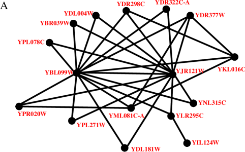
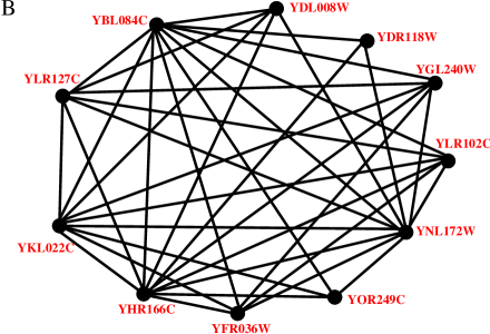
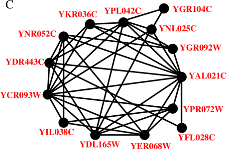
Figure 7: Examples of proteins clusters identified according to the community structure of figure 6.

The first example is a cluster which appears at resolution threshold $18.04$. It contains $16$ proteins and $33$ edges, and has the structure shown in figure 7A. This cluster is stable, namely that each vertex in it is more connected to vertices in this cluster than to vertices outside; and it has no further subcommunity structure. According to the protein interaction databank Xenarios et al. (2000); Bairoch and Apweiler (2000), $15$ of these proteins are all involved in ATP synthesis process in yeast. They may form a very important part of yeast’s mitochondrial ATPase complex. One protein of this cluster, YIL124W, is a hypothetical membrane protein. Because this last protein has only one interaction with other members of the cluster, it may not have similar biological functions as the other members.

The second example is a cluster which appears at resolution threshold $5.11$. It contains $11$ proteins and $38$ edges, and has the structure shown in figure 7B. This cluster is also stable and has no further structure. According to the protein interaction databank Xenarios et al. (2000); Bairoch and Apweiler (2000), among these $11$ proteins, YBL084C, YFR036W, YHR166C, YKL022C are known to be cell division control proteins; YGL240W plays a role in cell cycle and mitosis; YDR118W, YNL172W, YOR249C probably are membrane proteins; and YLR127C, YDL008W, YLR102C are hypothetical proteins whose functions remain to be determined. It is quite likely that all the proteins in this cluster are closely involved in cell division and membrane fission process. We anticipate that the three hypothetical proteins of this cluster will also have similar biological functions.

The third example is a cluster which appears only when the resolution threshold is refined to below $0.88$. It contains $14$ proteins and $41$ protein-protein interactions. This cluster is also stable and has no further structure. The interaction pattern of this cluster is demonstrated in figure 7C. Among these $14$ proteins, according to the protein interaction databank Xenarios et al. (2000); Bairoch and Apweiler (2000), YCR093W, YPR072W, YDL165W, YER068W, YIL038C are general negative regulator of transcription subunits; YAL021C is a glucose-repressible alcohol dehydrogenase transcriptional effector; YNR052C is a ubiquitous transcription factor; YDR443C, YGR104C are suppressors of RNA polymerases; YNL025C is the RNA polymerase II holoenzyme cyclin-like subunit; YPL042C is the meiotic mRNA stability protein kinase UME5; YGR092W is the cell cycle protein kinase DBF2; and YKR036C and YFL028C are two hypothetical proteins. It is quite likely that this cluster is mainly involved in RNA transcription process and we also anticipate that the two hypothetical proteins of this cluster are strongly related with this biological function.

To conclude this subsection, we stress that, based on the community structure of figure 6 many clusters of proteins can be constructed. Here we have mentioned just three examples. These identified protein clusters could help researchers to assign possible biological functions to hypothetical proteins, and could also suggest possible proteins that may be involved in carrying out a particular biological reaction.

V conclusion and discussion

In our earlier work zho (a), the distance between two vertices of a graph is defined as the average number of steps a Brownian particle takes to move from one vertex to the other. Based on this distance measure, in the present work we define a dissimilarity index to signify to what extent two nearest-neighboring vertices will be different from each other. We observe that vertices belonging to the same group usually have very small dissimilarity indices between them, while vertices of different communities usually have large dissimilarity indices between them. The observation leads naturally to an algorithm of network clustering. We applied this method to several artificial networks and also to different real networks in social and biological systems and satisfactory results are obtained. Different clusters of a network obtained by our method are characterized by a range of resolution threshold.

The examples studied by us in this paper suggest that our algorithm is very promising in identifying the community structure of a complex networked system. Why it works? Maybe it is because of the following reasons. First, the vertex-vertex distance measure has taken into account the topological structure of the network as well as the local connections of the network. The distances from one vertex to all the other vertices of the network actually give a perspective of the whole network viewed from this vertex. Second, the dissimilarity index defined by equation (1) compares the perspectives viewed from two nearest-neighboring vertices. It is intuitively appealing to assume that the perspectives of the different vertices of the same community are similar to each other while those of vertices of different communities will be quite different.

It is anticipated that the present work will find applications in the field of complex networks, as well as in the fields of sociological and biological sciences.

References

- Uetz et al. (2000) P. Uetz, L. Giot, G. Cagney, T. A. Mansfield, R. S. Judson, J. R. Knight, D. Lockshon, V. Narayan, M. Srinivasan, P. Pochart, et al., Nature (London) 403, 623 (2000).
- Wasserman and Faust (1994) S. Wasserman and K. Faust, Social Network Analysis: Methods and Applications (Cambridge University Press, UK, 1994).
- Ravasz et al. (2002) E. Ravasz, A. L. Somera, D. A. Mongru, Z. N. Oltvai, and A.-L. Barabási, Science 297, 1551 (2002).
- Girvan and Newman (2002) M. Girvan and M. E. J. Newman, Proc. Natl. Acad. Sci. U.S.A. 99, 7821 (2002).
- Freeman (1977) L. C. Freeman, Sociometry 40, 35 (1977).
- zho (a) H. Zhou (2003), Phys. Rev. E (to appear); eprint e-print: cond-mat/0302030.
- Flake et al. (2000) G. W. Flake, S. Lawrence, and C. L. Giles, in Proceedings of the Sixth International Conference on Knowledge Discovery and Data Mining (ACM SIGKDD-2000) (2000), pp. 150–160.
- zho (b) http://www.mpikg-golm.mpg.de/th/people/zhou/ NetworkCommunity.html.
- Zachary (1977) W. W. Zachary, J. Anthropol. Res. 33, 452 (1977).
- Xenarios et al. (2000) I. Xenarios, D. W. Rice, L. Salwinski, M. K. Baron, E. M. Marcotte, and D. Eisenberg, Nucleic Acids Res. 28, 289 (2000).
- Deane et al. (2002) C. M. Deane, L. Salwinski, I. Xenarios, and D. Eisenberg, Mol. Cell. Proteomics 1, 349 (2002).
- Bairoch and Apweiler (2000) A. Bairoch and R. Apweiler, Necleic Acids Res. 28, 45 (2000).