Network Landscape from a Brownian Particle’s Perspective

Abstract

Given a complex biological or social network, how many clusters should it be decomposed into? We define the distance $d_{i,j}$ from node $i$ to node $j$ as the average number of steps a Brownian particle takes to reach $j$ from $i$. Node $j$ is a global attractor of $i$ if $d_{i,j}\leq d_{i,k}$ for any $k$ of the graph; it is a local attractor of $i$, if $j\in E_{i}$ (the set of nearest-neighbors of $i$) and $d_{i,j}\leq d_{i,l}$ for any $l\in E_{i}$. Based on the intuition that each node should have a high probability to be in the same community as its global (local) attractor on the global (local) scale, we present a simple method to uncover a network’s community structure. This method is applied to several real networks and some discussion on its possible extensions is made.

A complex networked system, such as an organism’s metabolic network and genetic interaction network, is composed of a large number of interacting agents. The complexity of such systems originates partly from the heterogeneity in their interaction patterns, aspects of which include the small-world Watts and Strogatz (1998) and the scale-free properties Barabási and Albert (1999); Faloutsos et al. (1999) observed in many social, biological, and technological networks Strogatz (2001); Albert and Barabási (2002); Dorogovtsev and Mendes (2002). Given this high degree of complexity, it is necessary to divide a network into different subgroups to facilitate the understanding of the relationships among different components Girvan and Newman (2002); Ravasz et al. (2002).

A complex network could be represented by a graph. Each component of the network is mapped to a vertex (node), and the interaction between two components is signified by an edge between the two corresponding nodes, whose weight is related to the interaction strength. The challenge is to dissect this graph based on its connection pattern. We know that to partition a graph into two equally sized subgroups such that the number of edges in between reaches the absolute minimum is already a NP-complete problem, a solution is not guaranteed to be found easily; however it is still a well-defined question. On the other hand, the question $``$How many subgroups should a graph be divided into and how?” is ill-posed, as we do not have an objective function to optimize; and we have to rely on heuristic reasoning to proceed.

If we are interested in identifying just one community that is associated with a specified node, the maximum flow method Ford and Fulkerson (1979) turns out to be efficient. Recently, it is applied to identifying communities of Internet webpages Flake et al. (2000). An community thus uncovered is usually very small; and for this method to work well one needs a priori knowledge of the network to select the source and sink nodes properly. Another elegant method is based on the concept of edge betweenness Freeman (1977). The degree of betweenness of a edge is defined as the total number of shortest paths between pair of nodes which pass through it. By removing recursively the current edge with the highest degree of betweenness, one expects the connectivity of the network to decrease the most efficiently and minimal cutting operations is needed to separate the network into subgroups Girvan and Newman (2002). This idea of Girvan and Newman Girvan and Newman (2002) could be readily extended to weighted graphs by assigning each edge a length equalling its reciprocal weight. Furthermore, in the sociology literature, there is a relatively long tradition in identifying communities based on the criteria of reachability and shortest distance (see, e.g., Wasserman and Faust (1994)).

In this paper, a new method of network community identification is described. It is based on the concept of network Brownian motion: If an intelligent Brownian particle lives in a given network for a long time,what might be its perspective of the network’s landscape? We suggest that,without the need to removing edges from the network, the node-node distances $``$measured” by this Brownian particle can be used to construct the community structure and to identify the central node of each community. This idea is tested on several social and biological networks and satisfiable results are obtained. Several ways are discussed to extend and improve our method.

Consider a connected network of $N$ nodes and $M$ edges. Its node set is denoted by $V=\{1,\cdots,N\}$ and its connection pattern is specified by the generalized adjacency matrix $A$. If there is no edge between node $i$ and node $j$, $A_{ij}=0$; if there is an edge in between, $A_{ij}\equiv A_{ji}>0$ and its value signifies the interaction strength (self-connection is allowed). The set of nearest-neighbors of node $i$ is denoted by $E_{i}$. A Brownian particle keeps moving on the network, and at each time step it jumps from its present position (say $i$) to a nearest-neighboring position ($j$). When no additional knowledge about the network is known, it is natural to assume the following jumping probability $P_{ij}=A_{ij}/\sum_{l=1}^{N}A_{il}$ (the corresponding matrix $P$ is called the transfer matrix). One verifies that at time $t\gg M$ the probability $\rho(k)$ for the Brownian particle to be at any node $k$ is nonvanishing and equals to $\sum_{l}A_{kl}/\sum_{m,n}A_{mn}$, proportional to the total interaction capacity $\sum_{l}A_{kl}$ of node $k$.

Define the node-node distance $d_{i,j}$ from $i$ to $j$ as the average number of steps needed for the Brownian particle to move from $i$ through the the network to $j$. From some simple linear-algebra calculation Kolman (1973) it is easy to see that

$$d_{i,j}=\sum_{l=1}^{N}\left({1\over I-B(j)}\right)_{il},$$ (1)

where $I$ is the $N\times N$ identity matrix, and matrix $B(j)$ equals to the transfer matrix $P$ except that $B_{lj}(j)\equiv 0$ for any $l\in V$. The distances from all the nodes in $V$ to node $j$ can thus be obtained by solving the linear algebraic equation $[I-B(j)]\{d_{1,j},\cdots,d_{N,j}\}^{T}=\{1,\cdots,1\}^{T}$. We are mainly interested in sparse networks with $M=O(N)$; for such networks there exist very efficient algorithms Tewarson (1973); Davis and Duff (1999) to calculate the root of this equation. If node $j$ has the property that $d_{i,j}\leq d_{i,k}$ for any $k\in V$, then $j$ is tagged as a global attractor of node $i$ ($i$ is closest to $j$ in the sense of average distance). Similarly, if $j\in E_{i}$ and $d_{i,j}\leq d_{i,l}$ for any $l\in E_{i}$, then $j$ is an local attractor of $i$ ($i$ is closest to $j$ among all its nearest-neighbors). We notice that, in general the distance from $i$ to $j$ ($d_{i,j}$) differs from that from $j$ to $i$ ($d_{j,i}$). Consequently, if $j$ is an attractor of $i$, node $i$ is not necessarily also an attractor of $j$.

If a graph is divided into different subgroups, on the local scale we intuitively expect that each node $i$ will have a high probability to be in the same subgroup as its local attractor $j$, since among all the nearest-neighboring nodes in $E_{i}$, node $j$ has the shortest $``$distance” from node $i$. For simplicity let us just assume this probability to be unity (a possible improvement is discussed later). Thus, we can define a local-attractor-based community (or simply a $``$L-community”) as a set of nodes $L=\{i_{1},\cdots,i_{m}\}$ such that (1) if node $i\in L$ and node $j$ is an local attractor of $i$, then $j\in L$, (2) if $i\in L$ and node $k$ has $i$ as its local attractor,then $k\in L$, and (3) any subset of $L$ is not a L-community. Clearly, two L-communities $L_{a}$ and $L_{b}$ are either identical ($L_{a}\equiv L_{b}$) or disjoint ($L_{a}\cap L_{b}=\emptyset$). Based on each node’s local attractor the graph could be decomposed into a set of L-communities.

According to the same intuitive argument, on the global scale we expect that each node will have a high probability to be in the same community as its global attractor, and if assume this probability to be unity we can similarly construct the global-attractor-based communities ($``$G-communities”) based on the global-attractor of each node. For small networks, we expect the L- and G-community structures to be identical; while for large networks, each G-community may contain several L-communities as its subgroups. A community could be characterized by its size $N_{c}$ and an instability index $I_{c}$. A node $i$ in community $C$ is referred to as unstable if its total direct interaction with nodes in any another community $C^{\prime}$, $\sum_{k\in C^{\prime}}A_{ik}$, is stronger than its total direct interaction with other nodes in its own community, $\sum_{k\in C\backslash i}A_{ik}$. $I_{c}$ is the total number of such nodes in each community. We can also identify the center of a community (if it exists) as the node that is the global attractor of itself.

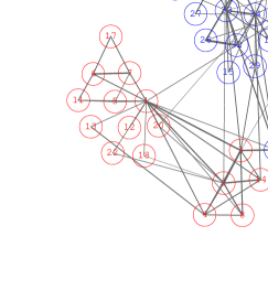
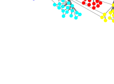
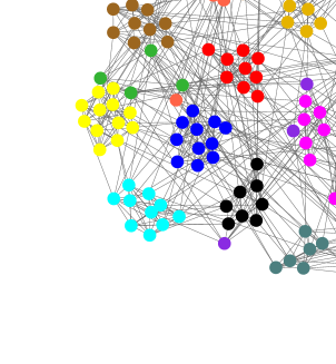
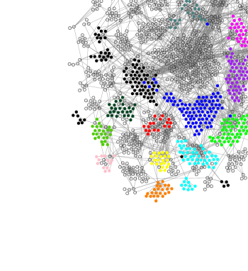
Figure 1: (Color) Community structure of some model networks (the nodes of the same L-community are spatially grouped together). (a) The karate club network compiled by Zachary Zachary (1977) (here nodes are colored according to their actual groupings); (b) the scientific collaboration network compiled by Girvan and Newman Girvan and Newman (2002); (c) the foot-ball match network compiled by Girvan and Newman Girvan and Newman (2002) (nodes are colored according to their actual groupings); and (d) the yeast protein interaction network Xenarios et al. (2000); Deane et al. (2002), here nodes of the same G-community are encoded with the same color (open circles denote nodes in $G_{1}$).

Now we test the above-mentioned simple method on some well-documented networks whose community structures are known. The first example is the social network recorded by Zachary Zachary (1977). This network contains $34$ nodes and $77$ weighted edges, and it was observed to spontaneously fission into two groups of size $16$ and $18$, respectively Zachary (1977) (these two groups are marked by two colors in Fig. 1A). The results of our method is shown in Fig. 1A. Community $L_{1}$ contains $11$ elements (node $13$ is unstable and has stronger direct interaction with $L_{2}$), $L_{2}$ has $6$ elements (node $9$ has stronger direct interaction with $L_{3}$), and $L_{3}$ has $17$ elements. Nodes $1$ (the manager), $3$, and $34$ (the officer) are the corresponding centers. We find that for this network the G-communities coincide with the L-communities.

As another example, the scientific collaboration network of Santa Fe Institute Girvan and Newman (2002) is considered. The giant connected component contains $118$ nodes and $200$ weighted edges, the weights are assigned according to the measure in Newman (2001). The present method divides the network into six L-communities, see Fig. 1B. All the nodes in community $L_{1}$ (size $14$), $L_{2}$ ($41$), $L_{4}$ ($8$), $L_{5}$ ($26$), and $L_{6}$ ($17$) are locally stable, and one node in $L_{3}$ has stronger direct interaction with community $L_{6}$. Same as the above example, the G-community structure is also identical to the L-community structure. Girvan and Newman divided this network into four major groups by recursively removing edges of highest degree of betweenness Girvan and Newman (2002): the largest of which was further divided into three subgroups and the second largest was divided into two subgroups. There are still some minor differences between the six subgroups obtained by the present method and those obtained in Girvan and Newman (2002), which may be attributed to the fact that, in the treatment of Girvan and Newman (2002) the network was regarded as unweighted.

The method is further tested on a relatively more complicated case, the foot-ball match network compiled by Girvan and Newman Girvan and Newman (2002). It contains $115$ nodes and $613$ unweighted edges. These $115$ teams were distributed into $12$ conferences by the game organizers. Based on the connection pattern, the present method divides them into $15$ L-communities, of which $11$ are locally stable: $L_{2}$ (size $9$), $L_{3}$ ($13$), $L_{4}$ ($14$), $L_{5}$ ($10$), $L_{6}$ ($8$), $L_{7}$ ($6$), $L_{8}$ ($7$), $L_{9}$ ($6$), $L_{10}$ ($4$), $L_{11}$ ($6$), and $L_{13}$ (size $9$). One element of $L_{1}$ (size $9$) has stronger interaction with $L_{10}$, and one element of $L_{12}$ (size $10$) has stronger interaction with $L_{3}$, and all the elements of $L_{14}$ (size $2$) and $L_{15}$ (size $2$) are locally unstable. The G-communities of this network are also identical to the L-communities. In Fig. 1C the community structure of this network is shown, where nodes belonging to each identified community are located together, and the different colors encode the actual $12$ conferences Girvan and Newman (2002). Figure  1C indicates that the predicted communities coincide very well with the actual communities. The community structure obtained by the present method is also in very good correspondence with that obtained by Girvan and Newman Girvan and Newman (2002) based on edge betweenness.

The above-studied networks all have relatively small network sizes and the identified G-communities coincide with the L-communities. Now we apply our method to the protein interaction network (yeast core Xenarios et al. (2000); Deane et al. (2002)) of baker’s yeast. The giant connected component of this network contains $1471$ proteins and $2770$ edges (assumed to be unweighted, since the interaction strengths between the proteins are generally undetermined). The present method dissect this giant component into $14$ G-communities (Table. 1) and into $69$ L-communities ($11$ of them contain one locally unstable node, $15$ of them have $2$-$7$ locally unstable nodes, all the others are stable). The relationship between the G- and L-communities is demonstrated in Fig 1D, where proteins are grouped into L-communities and those of the same G-community have the same color. We see from Fig. 1D that if two nodes are in the same L-community, they are very probable to be in the same G-community. The largest G-community ($G_{1}$) contains more than half of the proteins and is centered around nucleoporin YMR047C, which, according to SWISS-PROT description Bairoch and Apweiler (2000), is $``$an essential component of nuclear pore complex” and $``$may be involved in both binding and translocation of the proteins during nucleocytoplasmic transport”. YMR047C interact directly only with $39$ other proteins (it is even not the most connected node in the system), but associated with it is a group of $935$ proteins as suggested by the present method. The protein interaction network may be evolved to facilitate efficient protein transportation by protein-mediated indirect interactions.

What will happen if the protein YMR047C is removed from the network? The resulting perturbed system has $1463$ nodes and $2729$ edges, and we find that its L-community structure does not change much. Altogether $72$ L-communities are identified, and most of them contain more or less the same set of elements as in the unperturbed network. However, there is a dramatic change in the G-community structure. There are now $21$ G-communities (the largest of which has $574$ proteins), while $G_{1}$ of the original system breaks up into eight smaller G-communities. It was revealed that the most highly connected proteins in the cell are the most important for its survival, and mutations in these proteins are usually lethal Jeong et al. (2001). Our work suggests that, these highly connected proteins are especially important because they help integrating many small functional modules (L-communities) into a larger unit (G-community), enabling the cell to perform concerted reactions in response to environment stimuli.

In the above examples, the network studied are all from real-world. We have also tested the performance of our method to some artificial networks generated by computer. To compare with the result of Ref. Girvan and Newman (2002), we generated an ensemble of random graphs with $128$ vertices. These vertices are divided into four groups of $32$ vertices each. Each vertex has on average $16$ edges, $z_{\rm out}$ of which are to vertices of other groups, and the remaining are to vertices within its group; all these edges are drawn randomly and independently in all the other means. Using the method of Girvan and Newman, it was reported Girvan and Newman (2002) that when $z_{\rm out}<6$ all the vertices could be classified with high probability. Our present method in its simplest form could work perfectly only when $z_{\rm out}<2.5$. In the artificial network, the vertices are identical with each other in the statistical sense and there is no correlation between the degrees of two neighboring edges. Our method seems not to be the best for such kind of random networks.

In summary, we have suggested a simple way of grouping a graph of nodes and edges into different subgraphs based on the node-node distance measured by a Brownian particle. The basic idea was applied to several real networked systems and very encouraging results were obtained. The concept of random walking was also used in some recent efforts to facilitate searching on networks (see, e.g., Tadić (2002); Guimerà et al. (2002)), the present work may be the first attempt in applying it on identifying network community structure. Some possible extensions of our method are immediately conceivable: First, in the present work we have assumed that a node will be in the same community as its attractor with probability $1$. Naturally, we can introduce a $``$inverse temperature” $\beta$ and suppose that node $i$ be in the same community as node $j$ with probability proportional to $\exp(-\beta d_{i,j})$. The present work discusses just the zero temperature limit. We believe that the communities identified at zero temperature will persist until the temperature is high enough. Second, we can construct a gross-grained network by regarding each L-community as a single node, and defining the distance from one L-community to another as the average node-node distance between nodes in these two communities. The present method can then be applied, and the relationship between different L-communities can be better understood. Third, for very large networks, it is impractical to consider the whole network when calculating node-node distance. Actually this is not necessary, since the length of the shortest path between a given node and its attractor should be small. We can therefore focus on a localized region of the network to identify the attractor of a given node.

Furthermore, based on the distance measure of the present paper, we can define a quantity called the dissimilarity index for any two nearest-neighboring nodes. Nearest-neighboring vertices of the same community tend to have small dissimilarity index, while those belonging to different communities tend to have high dissimilarity index. Extensions of the present work will be reported in a forthcoming paper zhou2003 .

An interesting task is to use extended versions of the present method to explore the landscape of the Internet’s autonomous system Faloutsos et al. (1999) and that of the metabolic network of E. coli Selkov Jr et al. (1998); Ravasz et al. (2002).

I am grateful to M. Girvan and M. E. J. Newman for sharing data and to Professor R. Lipowsky for support.

Table 1: G-communities of yeast’s protein interaction network Xenarios et al. (2000); Deane et al. (2002). $N_{c}$ is the community size, $I_{c}$ is the number of locally unstable nodes.

index	$N_{c}$	$I_{c}$	center	index	$N_{c}$	$I_{c}$	center
$G_{1}$	$935$	$7$	YMR047C	$G_{8}$	$52$	$1$	YBR109C
$G_{2}$	$90$	$3$	YNL189W	$G_{9}$	$37$	$1$	YGR218W
$G_{3}$	$17$	$4$	YER148W	$G_{10}$	$19$	$2$	YML109W
$G_{4}$	$57$	$5$	YFL039C	$G_{11}$	$26$	$0$	YDR167W
$G_{5}$	$97$	$3$	YDR388W	$G_{12}$	$24$	$0$	YDL140C
$G_{6}$	$59$	$0$	YJR022W	$G_{13}$	$13$	$0$	YOL051W
$G_{7}$	$22$	$0$	YDR448W	$G_{14}$	$23$	$0$	YJR091C

References

- Watts and Strogatz (1998) D. J. Watts and S. H. Strogatz, Nature (London) 393, 440 (1998).
- Barabási and Albert (1999) A.-L. Barabási and R. Albert, Science 286, 509 (1999).
- Faloutsos et al. (1999) M. Faloutsos, P. Faloutsos, and C. Faloutsos, Comput. Commun. Res. 29, 251 (1999).
- Strogatz (2001) S. H. Strogatz, Nature (London) 410, 268 (2001).
- Albert and Barabási (2002) R. Albert and A.-L. Barabási, Rev. Mod. Phys. 74, 47 (2002).
- Dorogovtsev and Mendes (2002) S. N. Dorogovtsev and J. F. F. Mendes, Adv. Phys. 51, 1079 (2002).
- Girvan and Newman (2002) M. Girvan and M. E. J. Newman, Proc. Natl. Acad. Sci. U.S.A. 99, 7821 (2002).
- Ravasz et al. (2002) E. Ravasz, A. L. Somera, D. A. Mongru, Z. N. Oltvai, and A.-L. Barabábasi, Science 297, 1551 (2002).
- Ford and Fulkerson (1979) L. Ford and D. Fulkerson, Flows in networks (Princeton University Press, Princeton, New Jesey, 1979).
- Flake et al. (2000) G. W. Flake, S. Lawrence, and C. L. Giles, in Proceedings of the Sixth International Conference on Knowledge Discovery and Data Mining (ACM SIGKDD-2000) (2000), pp. 150–160.
- Freeman (1977) L. C. Freeman, Sociometry 40, 35 (1977).
- Wasserman and Faust (1994) S. Wasserman and K. Faust, Social Network Analysis: Methods and Applications (Cambridge University Press, UK, 1994).
- Kolman (1973) B. Kolman, Elementary Linear Algebra (4th Edition) (MacMillan Publisher, HB, 1986).
- Tewarson (1973) R. P. Tewarson, Sparse Matrices (Academic Press, New York, 1973).
- Davis and Duff (1999) T. A. Davis and I. S. Duff, ACM Trans. Math. Software 25, 1 (1999).
- Zachary (1977) W. W. Zachary, J. Anthropol. Res. 33, 452 (1977).
- Newman (2001) M. E. J. Newman, Phys. Rev. E 64, 016132 (2001).
- Xenarios et al. (2000) I. Xenarios, D. W. Rice, L. Salwinski, M. K. Baron, E. M. Marcotte, and D. Eisenberg, Nucleic Acids Res. 28, 289 (2000).
- Deane et al. (2002) C. M. Deane, L. Salwinski, I. Xenarios, and D. Eisenberg, Mol. Cell. Proteomics 1, 349 (2002).
- Bairoch and Apweiler (2000) A. Bairoch and R. Apweiler, Necleic Acids Res. 28, 45 (2000).
- Jeong et al. (2001) H. Jeong, S. P. Mason, A.-L. Barabási, and Z. N. Oltvai, Nature (London) 411, 41 (2001).
- Tadić (2002) B. Tadić, Eur. Phys. J. B 23, 221 (2002).
- Guimerà et al. (2002) R. Guimerà, A. Diaz-Guilera, F. Vega-Redondo, A. Cabrales, and A. Arenas, Phys. Rev. Lett. 89, 248701 (2002).
- (24) H. Zhou (2003), in preparation.
- Selkov Jr et al. (1998) E. Selkov Jr, Y. Grechkin, N. Mikhailova, and E. Selkov, Nucleic Acid Res. 26, 43 (1998).