Magneto-optical rotation of spectrally impure fields and its nonlinear dependence on optical density

Abstract

We calculate magneto-optical rotation of spectrally impure fields in an optical thick cold atomic medium. We show that the spectral impurity leads to nonlinear dependence of the rotation angle on optical density. Using our calculations, we provide a quantitative analysis of the recent experimental results of G. Labeyrie et al. [Phys. Rev. A 64, 033402 (2001)] using cold Rb⁸⁵ atoms..

I Introduction

A very useful way to get important spectroscopic information is by measuring magneto-optical rotation (MOR) of a plane polarized light propagating through a medium rmp . Clearly it is desirable to obtain as large an angle of rotation as possible conn ; gsa . It is known that the angle of rotation is proportional to the density of the medium. Thus an increase in density will help in achieving large rotation angles. Recently, very large rotation angles in a cold sample have been reported kaiser . In this experiment, optical densities of the order of $10-20$ were achieved. This experiment also reported a very interesting result, viz., the departure from the linear dependence of the rotation angle on the optical density. This departure has been ascribed to the nonmonochromatic nature of the input laser. The findings of the experiment warrant a quantitative analysis of the dependence of the rotation angle on the spectral profile of the input laser. We present a first principle calculation of this dependence. Note that a nonlinear dependence on optical density cannot result from a simple argument based on the standard formula for the rotation angle $\theta$:

$$\theta=\pi kl\;\textrm{Re}(\chi_{-}-\chi_{+})\;,$$ (1)

where, $k$ is the wave-number of the electric field, $l$ is the length of the medium, and $\chi_{\pm}$ represent the linear susceptibilities of the medium for right or left circularly polarized components of the input field. Since $\chi_{\pm}$ are proportional to the number density, the rotation angle becomes proportional to the optical density $\alpha$ defined by

$$\alpha=\frac{3\lambda^{2}}{2\pi}Nl\;,$$ (2)

where, $\lambda=2\pi/k$ is the wavelength of the input field, $N$ is the number density of the atomic medium. If one were to argue that spectrally impure laser field would replace $\chi_{\pm}$ by their averages over the width of the laser, then $\theta$ would continue to be proportional to the optical density $\alpha$. A more quantitative analysis of the rotation angle is thus warranted.

The organization of the paper is as follows. In Sec. II, we recapitulate the relevant equations for studies of MOR in atomic medium. In Sec. III, we describe a simple three-level atomic configuration in the context of MOR and discuss the effect of laser line-shape and magnetic field in a thick atomic medium. In Sec. IV, we consider experimental configuration used in kaiser . We show, how in an optically thick medium, one deviates from the linear dependence of rotation on optical density as a result of the spectral impurity of the laser field. We give a quantitative analysis of the experimental data.

II Basic equations

Let us consider that an atomic medium of length $l$ is resonantly excited by a monochromatic $\hat{x}$-polarized electric field

$$\vec{E}(z,t)=\hat{x}{\cal E}e^{ikz-i\omega t}+\textrm{c.c.}\;,$$ (3)

where, ${\cal E}$ is the field amplitude and $k=\omega/c=2\pi/\lambda$ is the wave number of the field, $\omega$ and $\lambda$ being the corresponding angular frequency and wavelength. The field is propagating in $z$-direction. Clearly, we can resolve the amplitude of the electric field into its two circular components as

$$\hat{x}{\cal E}\equiv\hat{{\epsilon}}_{+}{\cal E}_{+}+\hat{{\epsilon}}_{-}{\cal E}_{-}\;,$$ (4)

where, ${\cal E}_{\pm}={\cal E}/\sqrt{2}$ are the amplitude components along two circular polarization $\hat{\epsilon}_{\pm}=(\hat{x}\pm i\hat{y})/\sqrt{2}$.

While passing through the atomic medium these two circular components behave differently due to the anisotropy of the medium. Let $\chi_{\pm}$ be the susceptibilities of the medium corresponding to the two circular components. The electric field at the exit face of the medium can be written as

$$\vec{E}(l,t) = \vec{\cal E}_{l}e^{ikz-i\omega t}+\textrm{c.c.}\;,$$

$$\vec{\cal E}_{l} = \left[\hat{\epsilon}_{+}{\cal E}_{+}e^{2\pi ikl\chi_{+}}+\hat{\epsilon}_{-}{\cal E}_{-}e^{2\pi ikl\chi_{-}}\right]\;,$$ (5)

where, we have assumed that the medium is dilute so that $|4\pi\chi_{\pm}|\ll 1$. In MOR, the polarization direction of the input electric field gets rotated due to the difference in their dispersions (phase shifts) in a non-attenuating medium. The electric field however, remains linearly polarized after passing through the medium. In the present case, because the atom interacts with near-resonant electric field, the two circular components suffer attenuation (given by the imaginary part of $\chi_{\pm}$) while propagating through the medium. Thus the medium, concerned here, is responsible for both dispersion and attenuation. We term the medium to be both circularly birefringent and circularly dichroic. The output electric field becomes elliptically polarized under the action of such a medium. Thus to fully characterize the polarization state of the output field, one has to use the Stokes parameters born . The four Stokes parameters for an electric field are designated by $S_{\alpha}$ ($\alpha=0,1,2,3$) and can be defined as follows:

$$S_{0} = I_{\parallel}+I_{\perp}\;,$$ (6a)

$$S_{1} = I_{\parallel}-I_{\perp}\;,$$ (6b)

$$S_{2} = I_{45^{o}}-I_{-45^{o}}\;,$$ (6c)

$$S_{3} = I_{\sigma_{+}}-I_{\sigma_{-}}\;,$$ (6d)

where, $I_{\hat{n}}$ is the measured intensity along the polarization direction $\hat{n}$. Then the output polarization state can be characterized by the following three quantities:

$$P = \frac{\sqrt{S_{1}^{2}+S_{2}^{2}+S_{3}^{2}}}{S_{0}}\;,$$ (7a)

$$\tan{2\theta} = \frac{S_{2}}{S_{1}}~{}~{}~{}~{}(0\leqslant\theta<\pi)\;,$$ (7b)

$$\tan{2\phi} = \frac{S_{3}}{S_{0}P}~{}~{}~{}~{}(-\pi/4<\phi\leqslant\pi/4)\;,$$ (7c)

where, $P$ is the degree of polarization, i.e., the ratio of the intensities of the polarized component to the unpolarized one, $\theta$ is the Faraday rotation angle of the input field and is measured between the major axis of the ellipse and the $x$-axis, $\phi$ provides the ellipticity of polarization through the relation $e=\tan{\phi}$.

From Eq. (5) one can express the output intensities along different polarization directions in the following way:

$$I_{\parallel}(\omega) = |\hat{x}.\vec{\cal E}_{l}|^{2}=\frac{I_{o}}{4}|e^{2\pi ikl\chi_{+}}+e^{2\pi ikl\chi_{-}}|^{2}\;,$$ (8a)

$$I_{\perp}(\omega) = |\hat{y}.\vec{\cal E}_{l}|^{2}=\frac{I_{o}}{4}|e^{2\pi ikl\chi_{+}}-e^{2\pi ikl\chi_{-}}|^{2}\;,$$ (8b)

$$I_{\pm 45^{o}}(\omega) = \left|\frac{\hat{x}\pm\hat{y}}{\sqrt{2}}.\vec{\cal E}_{l}\right|^{2}$$ (8c)

$$= \frac{I_{o}}{8}|(1\pm i)e^{2\pi ikl\chi_{+}}+(1\mp i)e^{2\pi ikl\chi_{-}}|^{2}\;,$$

$$I_{\sigma_{\pm}}(\omega) = |\hat{\epsilon}_{\pm}.\vec{\cal E}_{l}|^{2}=\frac{I_{o}}{2}\exp{[-4\pi kl.\textrm{Im}(\chi_{\pm})]}\;,$$ (8d)

where, $I_{o}=|{\cal E}|^{2}$ is the input intensity of laser field.

Note that all the measured quantities defined by Eq. (8) are functions of the frequency of the exciting field. If the exciting field is spectrally impure, then the Stokes parameters $\langle S_{\alpha}\rangle$ are to be obtained by averaging over the spectrum $S(\omega)$ of the laser field. Thus, $I$’s in Eq. (6) are to be obtained from

$$\langle I_{\hat{n}}\rangle=\frac{1}{I_{o}}\int_{-\infty}^{\infty}d\omega I_{\hat{n}}(\omega)S(\omega)\;.$$ (9)

For simplicity, we can adopt, say, a Lorentzian line-shape for the input

$$S(\omega)\equiv I_{o}\frac{\gamma_{c}/\pi}{\gamma_{c}^{2}+(\omega-\omega_{l})^{2}}\;,$$ (10)

where, $\omega_{l}$ is the central frequency of the laser field and $2\gamma_{c}$ is the full width at half maximum. We will demonstrate how the fluctuations of the input field leads to the nonlinear dependence of the rotation angle on optical density.

Figure 1: Level diagram for a three-level configuration. The excited levels $|\pm\rangle$ ($m_{e}=\pm 1$) are Zeeman shifted from the level $m_{e}=0$ by an amount $s$. The detuning $\delta$ is defined between the levels $m_{e}=0$ and $m_{g}=0$.

III A simplified atomic model

We first consider a three-level atom in $V$ configuration (see Fig. 1) in order to uncover the effect of optical density on MOR. The levels $|\pm\rangle$ ($J_{e}=1,m_{e}=\pm 1$) are coupled to the ground state $|g\rangle$ ($J_{g}=0,m_{g}=0$) by two circular components $\sigma_{\pm}$ of $\hat{x}$-polarized electric field [Eq. (3)]. The excited level degeneracy has been removed by an uniform magnetic field $\vec{B}$ applied in the direction of propagation of the applied electric field. The levels $|e_{\pm}\rangle$ are shifted about line-center by an amount of $\mp\mu_{B}B/\hbar$ ($\mu_{B}$=Bohr magneton). The field $\vec{E}$ is detuned from the line center by an amount $\delta=\omega_{+g}(B=0)-\omega$, $\omega_{+g}(B=0)$ being the atomic transition frequency in absence of the magnetic field.

The susceptibilities of the $\sigma_{\pm}$ components inside the medium can be written as

$$\chi_{\pm}=\frac{N|\vec{d}|^{2}}{\hbar\gamma}\rho_{\pm};~{}~{}\rho_{\pm}=\frac{i\gamma}{\gamma+i(\delta\mp s)}\;,$$ (11)

where, $2\gamma=4|\vec{d}|^{2}\omega^{3}/3\hbar c^{3}$ is the spontaneous decay rate of the levels $|\pm\rangle$, $|\vec{d}|$ is the magnitude of the dipole moment vector for the transitions $|\pm\rangle\leftrightarrow|g\rangle$, $N$ is the atomic number density, and $s=\mu_{B}B/\hbar$ is the Zeeman splitting of the excited levels. Using these $\chi_{\pm}$, we can now write the field amplitude from Eq. (5) as

$$\vec{\cal E}_{0}=\left[\hat{\epsilon}_{+}{\cal E}_{+}e^{i\frac{\alpha}{2}\rho_{+}}+\hat{\epsilon}_{-}{\cal E}_{-}e^{i\frac{\alpha}{2}\rho_{-}}\right]\;,$$ (12)

where, $\alpha=4\pi klN|\vec{d}|^{2}/\hbar\gamma=(3\lambda^{2}/2\pi)Nl$ is the optical density of the medium.

Figure 2: Variation of MOR angle $\theta$ with optical density $\alpha$ for $s=2\gamma$ and different laser line-widths $\gamma_{c}=0.1\gamma$ (solid line), $\gamma_{c}=0.5\gamma$ (dashed line), $\gamma_{c}=\gamma$ (dot-dashed line), and $\gamma_{c}=2\gamma$ (long-dashed line). We have chosen $\lambda=422.67$ nm corresponding to Ca⁴⁰ 1S${}_{0}\leftrightarrow 1$P₁ transitions. Note the nonlinear dependence of $\theta$ on $\alpha$ for larger $\gamma_{c}$.

In what follows, we will assume that $\omega_{l}=\omega_{+g}(B=0)$. We calculate $\langle I_{\hat{n}}\rangle$’s using Eqs. (10) and (9) numerically for different values of $\gamma_{c}$ and $s$. We show the results in Fig. 2. We clearly see that for $\gamma_{c}\ll s$, the rotation angle $\theta$ is linearly proportional to $\alpha$. But for $\gamma_{c}\gtrsim s$, this variation deviates from linearity in large $\alpha$ domain. This behavior can be explained in terms of the off-resonant components which dominate for the large $\gamma_{c}$ and large $\alpha$.

In order to understand the numerical results, we first consider the limit of small optical densities whence

$$S_{1} = \frac{1}{2}[2+\alpha\textrm{Re}\{i(\rho_{+}+\rho_{-})\}]\;,$$ (13a)

$$S_{2} = \frac{\alpha}{2}\textrm{Re}(\rho_{-}-\rho_{+})\;.$$ (13b)

Thus, the departure of the rotation angle from the linearity has to do with the averages of the exponentials appearing in $I$’s [Eq. (8)]. If one were to make the approximation of replacing all $\chi$’s in Eq. (8) by their averages, i.e.,

$$\langle\exp{[2\pi ikl\chi_{\pm}]}\rangle\equiv\exp[2\pi ikl\langle\chi_{\pm}\rangle]\;,$$ (14)

then the Stokes parameters $\langle S_{1}\rangle$ and $\langle S_{2}\rangle$ would be

$$\langle S_{1}\rangle = e^{-\frac{\alpha}{2}(\langle\rho_{2}^{+}\rangle+\langle\rho_{2}^{-}\rangle)}\cos{\left[\frac{\alpha}{2}(\langle\rho_{1}^{+}\rangle-\langle\rho_{1}^{-}\rangle)\right]}\;,$$ (15a)

$$\langle S_{2}\rangle = -e^{-\frac{\alpha}{2}(\langle\rho_{2}^{+}\rangle+\langle\rho_{2}^{-}\rangle)}\sin{\left[\frac{\alpha}{2}(\langle\rho_{1}^{+}\rangle-\langle\rho_{1}^{-}\rangle)\right]}\;,$$ (15b)

where, $\langle\rho_{\pm}\rangle=\langle\rho_{1}^{\pm}\rangle+i\langle\rho_{2}^{\pm}\rangle$ and thus

Figure 3: Level diagram for the $F_{e}=4\leftrightarrow F_{g}=3$ transition. The numbers at the top of the figure indicate the magnetic quantum numbers of the sublevels. The relevant Clebsch-Gordan coefficients for the corresponding transitions are given by $a_{1}=-1/\sqrt{42},a_{2}=-\sqrt{5}/3\sqrt{14},a_{3}=-1/2\sqrt{21},a_{4}=-\sqrt{5}/2\sqrt{21},a_{5}=-1/6\sqrt{7},a_{6}=-1/2\sqrt{3},a_{7}=-1/3,a_{8}=-1/6,a_{9}=-1/\sqrt{21},a_{10}=-\sqrt{15}/6\sqrt{7},a_{11}=2/3\sqrt{7}$. The Zeeman splitting of the various sublevels are not shown.

$$\langle\theta\rangle=\frac{\alpha}{4}(\langle\rho_{1}^{-}\rangle-\langle\rho_{1}^{+}\rangle)=\frac{1}{2}.\frac{\alpha\gamma s}{(\gamma+\gamma_{c})^{2}+s^{2}}\;.$$ (16)

Clearly, the absorption does not contribute to the rotation angle. We have again recovered the linear dependence of $\theta$ on $\alpha$, provided the approximation (14) is valid. Thus, any departure in linearity of $\theta$ with respect to $\alpha$ indicates the breakdown the approximation (14). The numerical results of Fig. 2 clearly show the breakdown of the mean field description obtained by replacing $\chi$’s by their average values.

From the Eq. (16), we readily see that in the low $\alpha$-domain, by increasing $s$ (or $\gamma_{c}$) while keeping $\gamma_{c}$ (or $s$) constant, the slope of $\theta$ with $\alpha$ decreases. This is clear from the numerical results of Fig. 2. Also, for larger values of $\gamma_{c}$, variation of $\theta$ with $\alpha$ is deviated from linearity. Linear variation of $\theta$ with $\alpha$ is attributed to the monochromatic laser field. If the electric field is spectrally impure, then the off-resonant components also contribute to $\theta$, through the relations (9), (6), and (7). Thus, $\theta$ starts varying with $\alpha$ linearly in low $\alpha$ limit, then saturates, and finally decreases to zero to change the direction of rotation, for larger $\gamma_{c}$ (see Fig. 2). But for smaller $\gamma_{c}$, the linear behavior is retained even for larger $\alpha$, as the off-resonant components are not dominant in this parameter zone.

Figure 4: Variation of magneto-optical rotation angle $\theta$ with $\alpha$ for magnetic field (a) 2 Gauss ($\equiv 2\pi\times 2.8$ MHz) and (b) 8 Gauss ($\equiv 2\pi\times 11.2$ MHz) for laser line-widths $2\gamma_{c}=2\pi\times 0.5$ MHz (solid line), $2\gamma_{c}=2\pi\times 1$ MHz (dashed line), $2\gamma_{c}=2\pi\times 3$ MHz (dot-dashed line), and $2\gamma_{c}=2\pi\times 5$ MHz (long-dashed line). The dot-dashed curves correspond to the width of the laser used in the experiment kaiser . Note that the line-width of the D₂ line is $2\pi\times 5.88$ MHz.

Next we consider the variation of the degree of polarization $P$ and the ellipticity $e$ with $\alpha$. We have noticed that $P$ decreases from unity for increasing $\alpha$. This means that the output field no longer remains fully polarized, rather it becomes partially polarized.

Again, from the Eqs. (6d), (8d), and (11), it is clear that an integration over the entire range of detuning $\delta$ would yield $\langle S_{3}\rangle=0$, as the integrand is an odd function of $\omega$. Thus the ellipticity $e$ becomes zero. This means that the polarized part of the output field remains linear.

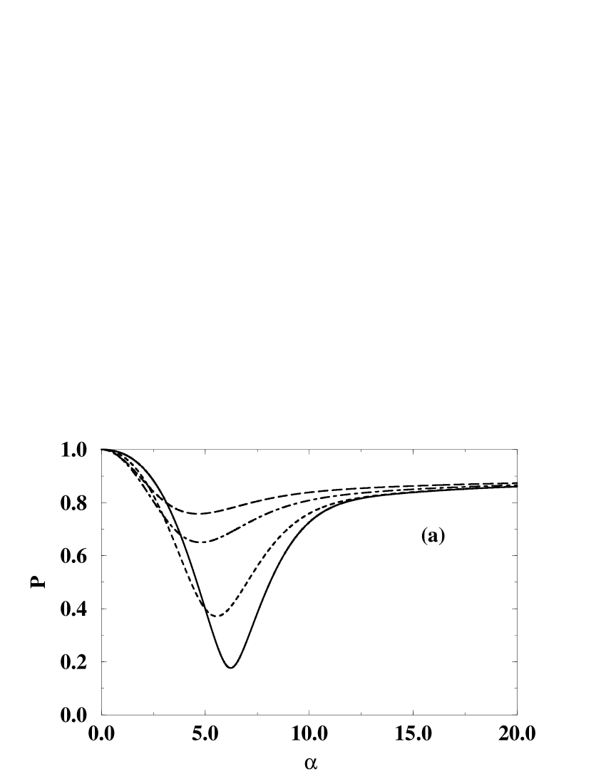
Figure 5: Variation of degree of polarization $P$ with $\alpha$ is shown for magnetic field (a) 2 Gauss and (b) 8 Gauss, for laser line-widths $2\gamma_{c}=2\pi\times 0.5$ MHz (solid line), $2\gamma_{c}=2\pi\times 1$ MHz (dashed line), $2\gamma_{c}=2\pi\times 3$ MHz (dot-dashed line), and $2\gamma_{c}=2\pi\times 5$ MHz (long-dashed line). The dot-dashed curves correspond to the width of the laser used in the experiment kaiser .

From the above discussion, it is clear that the output field gets rotated as a manifestation of cumulative effect of optical density, magnetic field, and laser line-width. Also it becomes partially polarized with no ellipticity.

IV Quantitative modeling of experimental results of Labeyrie et al. for MOR in spectrally impure fields

We now extend our understanding of resonant MOR as described in the previous section to explain the experimental data of Labeyrie et al.. In their experiment, a cold atomic cloud of Rb⁸⁵ is subjected to a static magnetic field. The laser probe beam passing through the medium in the direction of the magnetic field is tuned to the D₂ line of the atoms (2S${}_{1/2}\leftrightarrow$ 2P_3/2; $\lambda$=780.2 nm). They have measured the intensities of outputs with different polarizations, as function of laser detuning and also at different values of optical density. They have found a nonlinear dependence of the MOR angle $\theta$ on optical density. They found for larger magnetic field that the linear behavior is recovered.

To explain these observations, we consider the relevant energy levels of Rb⁸⁵ as used in the experiment (see Fig. 3). The $\hat{x}$-polarized electric field (3) is applied to cold Rb⁸⁵ medium near resonantly. The medium is subjected to uniform magnetic field $\vec{B}$ applied in the $z$-direction, i.e., along the direction of propagation of (3).

IV.1 Calculation of $\chi_{\pm}$ and optical density

The circular components $\sigma_{\pm}$ of the input electric field (3) interact with the transitions $m_{e}\leftrightarrow m_{g}=m_{e}-1$ and $m_{e}\leftrightarrow m_{g}=m_{e}+1$, respectively. We assume that the electric field is weak enough so that it is sufficient to use the linear response of the system to the laser field. We neglect the ground-state coherences. As we are considering the cold atoms, we neglect the collisional relaxations and Doppler broadening of the sublevels. We also assume that the atomic population is equally distributed over all the ground sublevels.

Using all these assumptions, we can write the susceptibilities $\chi_{\pm}$ for the $\sigma_{\pm}$ components as the sum of the susceptibilities of all the relevant $m_{e}\leftrightarrow m_{g}$ transitions in the following way:

$$\chi_{\pm}\equiv\sum_{m_{e},m_{g}}\frac{1}{7}\frac{N|\vec{d}_{m_{e},m_{g}}.\hat{\epsilon}_{\pm}|^{2}}{\hbar}.\frac{i}{\Gamma_{m_{e},m_{g}}+i(\delta+s_{m_{e},m_{g}})}\;,$$ (17)

where, $s_{m_{e},m_{g}}=(g_{g}m_{g}-g_{e}m_{e})s$ is the relative amount of Zeeman shift of the excited sublevel $m_{e}$ with respect to the Zeeman shifted ground sublevel $m_{g}$, $g_{g}=1/3$ and $g_{e}=1/2$ are the Landé-g factors of the ground and excited levels, respectively. The factor $1/7$ comes into the expression (17) as we have assumed equal population distribution in all the $(2F_{g}+1)=7$ ground sublevels. The coherence relaxation rate $\Gamma_{m_{e},m_{g}}$ in Eq. (17) is given by

$$\Gamma_{m_{e},m_{g}}=\frac{1}{2}\sum_{k}\gamma_{k,m_{e}}\;,$$ (18)

where, $\gamma_{i,j}$ is the spontaneous relaxation rate from the sublevel $j$ to $i$. Here we have assumed that there is no spontaneous relaxation from the ground sublevels. The terms $\vec{d}_{m_{e},m_{g}}$ and $\Gamma_{m_{e},m_{g}}$’s can be calculated from the relevant Clebsch-Gordan coefficients (see Fig. 3) sobel . The Einstein’s A coefficient for the D₂ line is known to be

$$A=\frac{4\omega^{3}}{3\hbar c^{3}}\frac{|(J=\frac{3}{2}\parallel D\parallel J^{\prime}=\frac{1}{2})|^{2}}{4}=\frac{4\omega^{3}}{3\hbar c^{3}}\frac{|(\frac{3}{2},\frac{5}{2},4\parallel D\parallel\frac{1}{2},\frac{5}{2},3)|^{2}}{9}\;,$$ (19)

where, $(~{}\parallel D\parallel~{})$ represents the reduced matrix element of the dipole moment vector $\vec{d}_{m_{e},m_{g}}$. The three symbols $3/2$, $5/2$, and $4$ correspond to $J$, $I$, and $F$ values respectively of the upper levels. Thus all $\Gamma_{m_{e},m_{g}}$’s in (17) are found to be equal to $(4\omega^{3}/3\hbar c^{3})|(\frac{3}{2},\frac{5}{2},4\parallel D\parallel\frac{1}{2},\frac{5}{2},3)|^{2}/2$.

We calculate the optical density $\alpha$ of the medium, when the input light field is resonant with $m_{e}=0\leftrightarrow m_{g}=0$ transition ($\delta=0$) in the absence of any magnetic field ($B=0$). For this, we first obtain the total output intensity from Eq. (6a) averaged by a very narrow laser line-shape, i.e., in the limit $\gamma_{c}\rightarrow 0$. Using Eq. (17), we thus find that the transmittivity of the medium becomes

$$T=\frac{1}{I_{o}}\langle S_{0}\rangle_{\gamma_{c}\rightarrow 0}=\frac{1}{I_{o}}S_{0}|_{\delta=0}=\exp(-\alpha)\;,$$ (20)

where, $\alpha=(3/7).(3\lambda^{2}/2\pi)Nl$. It should be borne in mind that it is different from the definition in Sec. III.

IV.2 Discussions

Using the above expressions of $\chi_{\pm}$ [Eq. (17)] and Eq. (9), we calculate the averaged intensities $\langle I_{\hat{n}}\rangle$ in different polarization directions. The Stokes parameters $S_{\alpha}$, degree of polarization $P$, and the Faraday rotation $\theta$ are calculated using the relations (7). In Fig. 4, we show how the Faraday angle $\theta$ varies with the optical density $\alpha$ for different values of $\gamma_{c}$ and $B$. Clearly, for $\gamma_{c}\ll s$, the rotation angle $\theta$ varies linearly with $\alpha$. But for larger $\gamma_{c}$ ($\gtrsim s$), the variation of $\theta$ with $\alpha$ deviates from linearity in large $\alpha$. This is because the off-resonant components contribute to the output intensity. Also, note that for a given value of $\gamma_{c}$, if $s$ is increased, the linearity is maintained even in the large $\alpha$-domain. This is because for larger $s$, the off-resonant components do not contribute much to the output intensity. The resonant frequency component is always dominant in the optical density range considered. We also note that, as $\gamma_{c}$ increases, the linear slope of $\theta$ with $\alpha$ decreases in the small $\alpha$ domain.

In Fig. 5, we show the variation of degree of polarization $P$ with $\alpha$ for various values of the $B$ and $\gamma_{c}$. These results reveal that with increase in $\alpha$, the degree of polarization deviates from unity, i.e., the output electric field not only rotates in polarization, but also it becomes partially polarized. However, the ellipticity of the output field still remains zero as we have argued in Sec. III.

V conclusions

In summary, we have given a quantitative analysis of magneto-optical rotation of spectrally impure fields in optically thick cold Rb⁸⁵ atomic medium. We have shown that the dependence of rotation on the optical density of the medium deviates from linearity due to the finite laser linewidth. Using our model, we explain the experimental results of Labeyrie et al..

References

• (1) D. Budker, W. Gawlik, D. F. Kimball, S. M. Rochester, V. V. Yashchuk, and A. Weis, Rev. Mod. Phys. 74, 1153 (2002).
• (2) J.-P. Connerade, J. Phys. B: At. Mol. Phys. 16, 399 (1983).
• (3) G. S. Agarwal, P. Anantha Lakshmi, J.-P. Connerade, and S. West, J. Phys. B: At. Mol. Opt. Phys. 30, 5971 (1997).
• (4) G. Labeyrie, C. Miniatura, and R. Kaiser, Phys. Rev. A 64, 033402 (2001).
• (5) M. Born and E. Wolf, Principles of Optics, 7th Ed. (Cambridge University Press, Cambridge, 1999), p. 630.
• (6) I. I. Sobel’man, Atomic Spectra and Radiative Transitions, 2nd Ed. (Springer Verlag, Berlin, 1992), Sec. 9.3.6.