SPONTANEOUS AND STIMULATED SYNCHROTRON RADIATION FROM RELATIVISTIC ELECTRONS IN ION CHANNEL

Abstract

Spontaneous and stimulated emission of an electron in the ion channel is studied. The emission processes are studied in the regime of high harmonic generation when the parameter of plasma wiggler strength is large. Like for conventional free electron laser, a synchrotron-like broadband spectrum is generated in this regime. The asymptotic expression for the radiation spectrum of the spontaneous emission is derived. The radiation spectrum emitted from axisymmetric monoenergetic electron beam is analyzed. The gain of ion-channel synchrotron-radiation laser is calculated. Use of laser-produced ion channel for efficient X-ray generation is discussed.

I Introduction

An electron dynamics in plasma-focusing channel has important applications to new plasma technologies, such as advanced accelerators esarey-review , novel radiation sources, new types of lens lens . It is a key phenomenon for ion-channel laser (ICL) ion channel laser , ion-ripple laser ion ripple laser , plasma-wiggler free electron laser(FEL) plasma fel , which are perspective candidates for high brightness X-ray radiation sources. Such radiation sources are strongly needed for experimental research in physics, chemistry, biology and in engineering light sources .

Resent experiments that explore the interaction of intense 28.5-GeV electron beam with plasma at Stanford Linear Accelerator Center (SLAC) wang ; joshi-review have shown that ion channel can be successfully used to produce broadband X-ray radiation. Moreover, the high density of the ions in the channel provides much higher wiggler strength than that provided by a conventional magnet wiggler. This leads to a more effective generation of X-ray radiation than in conventional light sources and could be used for the development of next generation of radiation sources.

To create ion channel, electron beam have to interact with plasma in blow-out regime blow-out regime when the electron beam density, $n_{b}$, is higher than plasma density, $n_{p}$. In this regime the electron beam charge quasistatically expels slow plasma electrons inside and around the beam volume and the ion channel is formed. Note that relativistic electrons of the beam are not expelled from the channel because of relativistic compensation of the beam electron charge force by the self-magnetic force book-beam . The channel radius, $r_{i}\simeq r_{0}\sqrt{n_{b}/n_{p}}$ is much more than electron beam radius, $r_{0}$, for dense $n_{b}\gg n_{p}$ and narrow $k_{p}r_{0}\ll 1$ electron beam beam radius , where $k_{p}=c/\omega_{p}$ is the plasma skin depth, $\omega_{p}=\left(4\pi n_{p}e^{2}/m\right)^{1/2}$ is the plasma frequency, $e$ is the electron charge, $m$ is the electron mass and $c$ is the speed of light. If all plasma electrons are expelled from the channel then the restoring force on the beam electrons due to the ion charge is given by Gauss’s low and in cylindrical geometry is:

$${\bf F}_{res}=m\omega_{p}^{2}{\bf r}_{\perp}/2,$$ (1)

where ${\bf r}_{\perp}$ is the vector from an electron to the channel axis. The beam electrons in the ion channel will undergo betatron oscillations caused by this force. The wavelength for small betatron oscillations is close to $\lambda_{b}=2\pi/k_{b}\simeq 2\pi\sqrt{2\gamma}/k_{p}$, where $\gamma$ is the relativistic factor of the electron beam betatron oscillations .

It is well known that accelerated charges emit electromagnetic (EM) radiation jackson . Therefore the electrons undergoing betatron oscillations in ion channel will emit short-wavelength EM radiation. Some features of this radiation spectrum have been studied in Ref.  wang ; joshi-review ; esarey1 . The wavelength of the radiation is close to $\lambda\simeq\lambda_{b}/\left(2\gamma^{2}\right)$ for small-amplitude near-axis betatron oscillations. If the amplitude of the betatron oscillations becomes large then electron radiates high harmonics. If the plasma wiggler strength,

$$K=\gamma k_{b}r_{0}=1.33\cdot 10^{-10}\sqrt{\gamma n_{e}\left[cm^{-3}\right]}r_{0}\left[\mu m\right],$$ (2)

is so high that $K\gg 1$ then radiation spectrum becomes quasi-continuous broadband, where $r_{0}$ is amplitude of electron betatron oscillation in the channel. The frequency dependence of the radiation spectrum becomes similar to the one of synchrotron radiation spectrum which is determined by the universal function

$$S\left(\omega/\omega_{c}\right)=\left(\omega/\omega_{c}\right)\int_{\omega/\omega_{c}}^{\infty}K_{5/3}\left(x\right)dx,$$ (3)

where $\omega_{c}$ is the critical frequency (see Fig. 1) jackson . For frequencies well below the critical frequency $\left(\omega\ll\omega_{c}\right)$ the spectrum increases with frequency as $\omega^{2/3}$, reaches a maximum at$\ \sim 0.29\omega_{c}$, and then drops exponentially to zero above $\omega_{c}$. The critical frequency for a relativistic electron in an ion channel is esarey1

$$\omega_{c}=\frac{3}{2}\gamma^{3}cr_{0}k_{b}^{2}=5.2\cdot 10^{-24}\gamma^{2}n_{e}\left[cm^{-3}\right]r_{0}\left[\mu m\right]keV.$$ (4)

Because of the strongly relativistic motion of the electron the emitted radiation is confined in very narrow angle $\theta\simeq K/\gamma$. Synchrotron radiation in ion channel has been observed in recent experiments wang .

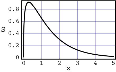
Figure 1: The synchrotron radiation function $S(x)$ versus $x$.

The averaged total power radiated by an electron undergoing betatron oscillations is esarey1

$$\left\langle P_{total}\right\rangle\simeq\frac{e^{2}c}{12}N_{b}\gamma^{2}k_{b}^{4}r_{0}^{2},$$ (5)

where $N_{b}$ is the number of the betatron oscillations performed by the electron. We can introduce also the stopping power of an electron, that is the energy loss of an electron per unit distance

$$Q=\left\langle P_{total}\right\rangle/c\simeq 1.5\cdot 10^{-45}\left(\gamma n_{e}\left[cm^{-3}\right]r_{0}\left[\mu m\right]\right)^{2}\frac{MeV}{cm}.$$ (6)

The averaged number of the photons with averaged energy $\hbar\omega_{c}$ is

$$\left\langle N_{ph}\right\rangle\simeq\frac{4\pi}{9}\frac{e^{2}}{\hbar c}N_{b}K\simeq 1.02\cdot 10^{-2}N_{b}K.$$ (7)

It follows from Eq. (5) that the radiated power is proportional to the squared density of ions in the channel. This fact has been confirmed in the experiments wang . As it was mentioned above the ion density in the channel have to be less than electron density in the beam. This leads to the serious limits on the gain in radiated power. One of the ways to overcome the limits is to use laser-produced ion channel. The ion density in such channel can be about $10^{19}cm^{-3}$ laser channel ; pukhov1 that is in 5 order higher than ion density in the channel produced in beam - plasma interaction experiments wang . So use of ion channel produced by laser pulse could increase the power of X-ray radiation in $10^{10}$ times! More detailed discussion on use of relativistic laser channel for X-ray generation will be presented in Conclusion.

Spontaneous emission in an ion channel has been studied in detail in Ref. esarey1 . The general expression for the spectrum has been derived. It is a complex expression that involves the sum of products of the Bessel function. Numerical evaluation of the spectrum becomes difficult in the limit $K\gg 1$. The simple asymptotic expression for the angular dependence of the radiated spectrum has been derived for this limit only for directions that are perpendicular to the plane of the betatron oscillation. The one of the purposes of our paper is to calculated the total angular dependence of the radiated spectrum.

Resonance interaction between EM radiation and the betatron oscillations of electron beam in ion channel leads to the bunching of the electron beam and then to the amplification (or damping) of EM radiation. It is a stimulated emission (or absorption). Stimulated emission is a basic process in ICLs ion channel laser and FELs book-fel . Reverse process - stimulated absorption leads to the direct laser acceleration pukhov DLA and to the magnetic field generation kostyukov IFE in relativistic laser channel. Unfortunately stimulated emission (absorption) in ion channel has not yet been explored in the limit $K\gg 1$ that is another objective of our paper.

The paper is organized as follows. In Section II the motion of an electron is studied and Hamiltonian formulation of the problem is presented. In Section III, the spontaneous emission from electrons undergoing betatron oscillations in ion channel is analyzed. The general asymptotic expression of the radiation spectrum for arbitrary angular dependence is derived for $K\gg 1$. The spectrum averaged over azimuthal angle is calculated for axially symmetrical electron beam in the limit $K\gg 1$. Section IV discusses the stimulated emission processes. The gain of ion - channel synchrotron - radiation laser is derived. A summary discussion is presented in Sec. V.

II Electron dynamics in ion channel

Relativistic equation of electron motion in cylindrical ion channel is

$$\frac{d{\bf p}}{dt}={\bf F}_{res},$$ (8)

where ${\bf F}_{res}$ is the restoring force defined by Eq. (1). It follows from Eq. (8) that momentum along channel axis $p_{z}$ is a constant of motion. First we will consider the radial betatron oscillation as it takes place when the center of an electron bunch moves along the channel axis. Assuming that $p_{y}=0$ we get the equation for $x$ -coordinate:

$$\frac{d^{2}x}{dt^{2}}=\frac{\gamma_{z}^{2}}{2\gamma^{3}}x,$$ (9)

where we introduce the constant of motion $\gamma_{z}^{2}=1+p_{z}^{2}$ and use the dimensionless units, normalizing the time to $\omega_{p}^{-1}$, the length to $c/\omega_{p}$, the momentum to $mc$.

As Hamiltonian does not depend on time it is another constant of motion

$$H=\gamma+\frac{x^{2}}{4}=const=\gamma_{z}+\frac{r_{0}^{2}}{4},$$ (10)

where $r_{0}$ is the amplitude of the betatron oscillation. We can express $\gamma$ as function of $x$ from the obtained relation to resolve Eq. (9). Then transversal motion of electron can be reduced to the oscillations in effective potential

$$U\left(x\right)=\frac{8\gamma_{z}^{2}}{\left(4\gamma_{z}+r_{0}^{2}-x^{2}\right)^{2}}.$$ (11)

The oscillations can be described in implicit form as follows

$$t = r_{0}\frac{\sqrt{\nu^{2}+4}}{\nu}E\left(arc\sin\left(\frac{x}{r_{0}}\right),\frac{\nu^{2}}{\nu^{2}+4}\right)$$ (12)

$$-\frac{2}{\nu\sqrt{\nu^{2}+4}}F\left(arc\sin\left(\frac{x}{r_{0}}\right),\frac{\nu^{2}}{\nu^{2}+4}\right),$$

where $E(x,k)$ and $F(x,k)$ are the Elliptic integrals of the first and the second kinds special function , respectively, and $\nu$ is

$$\nu^{2}=r_{0}^{2}/2\gamma_{z}.$$ (13)

The period of betatron oscillations is

$$T_{b}=\frac{2\pi}{\omega_{b}}=4r_{0}\frac{\sqrt{\nu^{2}+4}}{\nu}\left[E\left(\frac{\nu^{2}}{\nu^{2}+4}\right)-\frac{2}{\nu^{2}+4}K\left(\frac{\nu^{2}}{\nu^{2}+4}\right)\right],$$ (14)

where $K(x)$ and $E(x)$ are the complete Elliptic integrals of the first and the second kinds special function , respectively. In the limit $\nu^{2}\ll 1$, parameter $\nu$ is the ratio between the longitudinal and transversal energy of the electron

$$\nu^{2}\simeq p_{x}^{2}/\gamma_{z}^{2}\simeq p_{\perp}^{2}/p_{z}^{2},$$ (15)

where $p_{x}$ is the maximum of the transversal momentum which is at the channel axis $x=0$. In most applications transversal moment of the electron is much less than longitudinal one, so we assume that $\nu\ll 1$. Then we can use expansion in $\nu$ to describe betatron oscillations:

$$\omega_{b}=\frac{1}{\sqrt{2\gamma_{z}}}\left(1-\frac{3}{8}\nu^{2}+...\right),$$ (16)

$$x\left(t\right)=r_{0}\sin\left(\omega_{b}t\right)-r_{0}\frac{3}{64}\nu^{2}\sin\left(3\omega_{b}t\right)+....$$ (17)

Using Eq. (10) we obtain the relations for the electron orbit in the zeroth order in $\nu$ that coincides with ones calculated in Ref. esarey1

$$\omega_{b}\simeq\frac{1}{\sqrt{2\gamma_{z}}},$$ (18)

$$x\left(t\right)\simeq r_{0}\sin\left(\omega_{b}t\right),$$ (19)

$$y\left(t\right)\simeq 0,$$ (20)

$$z\left(t\right)\simeq z_{0}+\frac{p_{z}}{\gamma_{z}}\left(1-\frac{\nu^{2}}{4}\right)t-r_{0}\frac{p_{z}}{\gamma_{z}}\frac{\nu}{8}\sin\left(2\omega_{b}t\right).$$ (21)

Notice that parameter $\nu$ coincides with the expression $k_{b}r_{0}$ introduced in Ref. esarey1 and plasma wiggler strength parameter can be expressed through $\nu$ as $K\simeq\gamma_{z}\nu\simeq p_{\perp}$.

More general regime of the betatron motion when $p_{y}\neq 0$ and an electron orbit is not plane has been considered and classified in Ref. kostyukov IFE in the limit $p_{z}\gg p_{\perp}$. Equations of motion take a form in this case

$$x\left(t\right)\simeq\frac{p_{x}}{\sqrt{2\gamma_{z}}}\sin\left(\omega_{b}t\right),$$ (22)

$$y\left(t\right)\simeq\frac{p_{y}}{\sqrt{2\gamma_{z}}}\sin\left(\omega_{b}t+\psi\right),$$ (23)

$$z\left(t\right)\simeq z_{0}+\frac{p_{z}}{\gamma_{z}}\left[1-\frac{p_{x}^{2}+p_{y}^{2}}{4\gamma_{z}^{2}}-\frac{p_{x}^{2}}{8\gamma_{z}^{2}}\sin\left(2\omega_{b}t\right)+\frac{p_{y}^{2}}{8\gamma_{z}^{2}}\sin\left(2\omega_{b}t+2\psi\right)\right],$$ (24)

where $\psi$ is the phase difference between oscillations along $x$-axis and $y$-axis, $p_{x}$ and $p_{y}$ are the maximum of the electron momentum along $x$-axis and along $y$-axis, respectively, that occurs at the channel axis ($x=0$, $y=0$). If angular momentum of the electron, $L=p_{y}x-p_{x}y$ is equal to zero, then electron executes radial harmonic oscillations through the origin with amplitude $r_{0}=2\sqrt{H}$. If $L=\pm L_{\max}=\pm H/\omega_{b}$ then an electron performs circular motion with radius $r_{0}$. In the general case (an arbitrary value of $-L_{\max}<L<L_{\max}$) the electron trajectory is an ellipse-like and is confined between the maximal radius, $\sqrt{\left(H+\sqrt{H^{2}-\omega_{b}^{2}L^{2}}\right)}$, and minimal radius, $\sqrt{\left(H-\sqrt{H^{2}-\omega_{b}^{2}L^{2}}\right)}$.

III Spontaneous emission

Using Eqs. (22) - (24) for electron trajectory, the energy spectrum radiated by an electron can be calculated jackson ; esarey1 . The total radiation flux can be separated in two independent components with polarization in the ${\bf e}_{\theta}$ and ${\bf e}_{\phi}$ directions, where unit vectors ${\bf e}_{\theta}$ and ${\bf e}_{\phi}$ correspond to spherical coordinate system: $x=r\sin\theta\cos\phi$, $y=r\sin\theta\sin\phi$, $z=r\cos\theta$. Then energy radiated per frequency $\omega$ per solid angle in the direction ${\bf k}=\left(\omega/c\right)\left({\bf e}_{x}\sin\theta\cos\phi+{\bf e}_{y}\sin\theta\sin\phi+{\bf e}_{z}\cos\theta\right)$ during the interaction time $T$ is esarey1 :

$$\frac{dW_{spon,j}}{d\omega d\Omega}=\frac{e^{2}}{4\pi^{2}c}\eta^{2}\left|I_{j}\right|^{2},$$ (25)

$$I_{\theta}=\int\limits_{-T/2}^{T/2}\left(\frac{dx}{dt}\cos\theta\cos\phi+\frac{dy}{dt}\cos\theta\sin\phi-\frac{dz}{dt}\sin\theta\right)e^{i\Psi}dt,$$ (26)

$$I_{\phi}=\int\limits_{-T/2}^{T/2}\left(\frac{dx}{dt}\sin\phi-\frac{dy}{dt}\cos\phi\right)e^{i\Psi}dt,$$ (27)

$$\Psi=\eta\left[t-x\left(t\right)\sin\theta\cos\phi-y\left(t\right)\sin\theta\sin\phi-z\left(t\right)\cos\theta\right],$$ (28)

where $j=\theta,\phi$ is the polarization index, the electron trajectory is given by Eqs. (22) - (24) and $\eta=\omega/\omega_{p}$. The final results can be expressed as double infinite series of the Bessel function products (see Eqs. (32) - (41) in Ref. esarey1 or can be expressed by the infinite series of the generalized Bessel function introduced in quantum electrodynamics general Bessel ). Unfortunately the series converge slowly in the limit $K\gg 1$ that makes the numerical evaluation of the radiation spectrum difficult. Energy spectrum and angular dependence of radiation have been derived only for directions that are perpendicular to the plane of the betatron oscillation (i. e., for $\phi=\pi/2$) esarey1 . To extend this result we will use saddle point method saddle point to evaluate integrals (26) and (27).

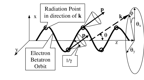
Figure 2: Schematic of synchrotron radiation in an ion channel. Open circles show the points on the electron trajectory when the electron emits in the direction of ${\bf k}$.

It is well known that radiation of accelerated relativistic electron is beamed in a very narrow cone in the direction of the electron momentum vector, and is seen by the observer as a short pulse of radiation as the searchlight beam sweeps across the observation point jackson (see Fig. 2). So the time moments when the electron momentum, ${\bf p}$, is directed along wave number, ${\bf k}$, give the main contribution in integrals ( 26) and (27). As the pulse duration is very short it is necessary to know the electron momentum and the electron position over only a small arc of the trajectory whose tangent points in the direction that is close to the direction of ${\bf k}$. Then we can expand integrand in Eqs. (26) and (27) about this time moments and perform integration. This approach implies that we approximate the part of the electron trajectory near these time moments by the arc of a circular path jackson . In this case the radiation will have well-known synchrotron-like spectrum. It is noted in Ref. landau that another necessary (the first is that the electron have to be relativistic) condition for use of the synchrotron radiation approach is that the electron deflection angle should be much more than simultaneous angle spread to which radiation is emitted. The electron momentum oscillates in cone angle $\sim p_{\perp}/p_{z}$ (electron deflection angle). The radiation of the relativistic particle is confined to angle $1/\gamma$ jackson . So the validity condition for synchrotron radiation approach is $p_{\perp}/p_{z}\gg 1/\gamma$ that is equivalent to the condition for high harmonics generation discussed in Introduction $K\gg 1$. Therefore the radiation spectrum can be approximated by the synchrotron one if

$$\gamma\gg p_{\perp}\gg 1.$$ (29)

This condition is easily satisfied in experiments.

The arguments presented above justify the use of the saddle point method saddle point to evaluate integrals (26) and (27). We can expand phase $\Psi$ about the moment of time $\xi_{n}=\omega_{b}t_{n}$ to the third order:

$$\Psi=\Psi_{0}+b_{1}(\xi-\xi_{n})+b_{2}(\xi-\xi_{n})^{2}+b_{3}(\xi-\xi_{n})^{3},$$ (30)

$$\Psi_{0} = \Psi\left(\xi_{n}\right)=\alpha_{0}\xi_{n}-\alpha_{x}\sin\left(\xi_{n}\right)-\alpha_{y}\sin\left(\xi_{n}+\psi\right)$$ (31)

$$+\alpha_{zx}\sin\left(2\xi_{n}\right)+\alpha_{zy}\sin\left(2\xi_{n}+2\psi\right),$$

$$b_{1} = \left.\frac{d\Psi}{d\xi}\right|_{\xi=\xi_{n}}=\alpha_{0}-\alpha_{x}\cos\left(\xi_{n}\right)-\alpha_{y}\cos\left(\xi_{n}+\psi\right)$$ (32)

$$+2\alpha_{zx}\cos\left(2\xi_{n}\right)+2\alpha_{zy}\cos\left(2\xi_{n}+2\psi\right),$$

$$b_{2} = \left.\frac{d^{2}\Psi}{d\xi^{2}}\right|_{\xi=\xi_{n}}=\alpha_{x}\sin\left(\xi_{n}\right)+\alpha_{y}\sin\left(\xi_{n}+\psi\right)$$ (33)

$$-4\alpha_{zx}\sin\left(2\xi_{n}\right)-4\alpha_{zy}\sin\left(2\xi_{n}+2\psi\right),$$

$$b_{3} = \left.\frac{d^{3}\Psi}{d\xi^{3}}\right|_{\xi=\xi_{n}}=\alpha_{x}\cos\left(\xi_{n}\right)+\alpha_{y}\cos\left(\xi_{n}+\psi\right)$$ (34)

$$-8\alpha_{zx}\cos\left(2\xi_{n}\right)-8\alpha_{zy}\cos\left(2\xi_{n}+2\psi\right),$$

where

$$\alpha_{0}=\frac{\eta}{\omega_{b}}\left[1-\frac{p_{z}}{\gamma_{z}}\left(1-\frac{p_{x}^{2}+p_{y}^{2}}{4\gamma_{z}^{2}}\sin\theta\cos\phi\right)\right],$$ (35)

$$\alpha_{x}=\frac{\eta}{\omega_{b}}\frac{p_{x}}{\gamma_{z}}\sin\theta\cos\phi,$$ (36)

$$\alpha_{y}=\frac{\eta}{\omega_{b}}\frac{p_{y}}{\gamma_{z}}\sin\theta\cos\phi,$$ (37)

$$\alpha_{zx}=\frac{\eta}{\omega_{b}}\frac{p_{z}}{\gamma_{z}}\frac{p_{x}^{2}}{8\gamma_{z}^{2}}\cos\theta,$$ (38)

$$\alpha_{zy}=\frac{\eta}{\omega_{b}}\frac{p_{z}}{\gamma_{z}}\frac{p_{y}^{2}}{8\gamma_{z}^{2}}\cos\theta.$$ (39)

Then we can expand the pre-exponent factors in Eqs. (26) and (27) about the moment of time $\xi_{n}=\omega_{b}t_{n}$ o the first order:

$$\frac{dx}{dt}\cos\theta\cos\phi+\frac{dy}{dt}\cos\theta\sin\phi-\frac{dz}{dt}\sin\theta=B_{\theta,n}+D_{\theta,n}(\xi-\xi_{n}),$$ (40)

$$\frac{dx}{dt}\sin\phi-\frac{dy}{dt}\cos\phi=B_{\phi,n}+D_{\phi,n}(\xi-\xi_{n}),$$ (41)

where

$$B_{\theta,n} = \left(\frac{p_{x}}{\gamma_{z}}\cos\xi_{n}\cos\phi+\frac{p_{y}}{\gamma_{z}}\cos\left(\xi_{n}+\psi\right)\sin\phi\right)\cos\theta$$ (42)

$$-\sin\theta\frac{p_{z}}{\gamma_{z}}\left[1-\frac{p_{x}^{2}}{4\gamma_{z}^{2}}\cos\left(2\xi_{n}\right)-\frac{p_{y}^{2}}{4\gamma_{z}^{2}}\cos\left(2\xi_{n}+2\psi\right)\right],$$

$$D_{\theta,n} = -\left[\frac{p_{x}}{\gamma_{z}}\sin\xi_{n}\cos\phi+\frac{p_{y}}{\gamma_{z}}\sin\left(\xi_{n}+\psi\right)\sin\phi\right]\cos\theta$$ (43)

$$-\frac{p_{z}}{\gamma_{z}}\frac{p_{x}^{2}}{2\gamma_{z}^{2}}\sin\theta\sin\left(2\xi_{n}\right)-\frac{p_{z}}{\gamma_{z}}\frac{p_{y}^{2}}{2\gamma_{z}^{2}}\sin\theta\sin\left(2\xi_{n}+2\psi\right),$$

$$B_{\phi,n}=\frac{p_{x}}{\gamma_{z}}\sin\phi\cos\left(\xi_{n}\right)-\frac{p_{y}}{\gamma_{z}}\cos\phi\cos\left(\xi_{n}+\psi\right),$$ (44)

$$D_{\phi,n}=-\frac{p_{x}}{\gamma_{z}}\sin\phi\sin\left(\xi_{n}\right)+\frac{p_{y}}{\gamma_{z}}\cos\phi\sin\left(\xi_{n}+\psi\right).$$ (45)

Notice that it is sufficient to keep the leading term in the pre-exponent factor while only terms that are much less than unity can be neglected in the exponent argument.

The main contribution to the integral comes from the neighborhood of the saddle points specified by $d\Psi/d\xi=0$ saddle point . The first-order term in phase expansion (30) can be written as follows

$$\left.\frac{d\Psi}{d\xi}\right|_{\xi=\xi_{n}}=\frac{\eta}{\omega_{b}}\left(1-\frac{{\bf k\cdot p}}{k\gamma}\right)\simeq\frac{\eta}{2\omega_{b}}\left(\frac{1}{\gamma^{2}}+\varphi^{2}\right),$$ (46)

where $\varphi$ is the angle between ${\bf k}$ and ${\bf p}$. It follows from Eq. (46) that $d\Psi/d\xi$ is minimal and close to zero at $\varphi=0$ when the electron momentum is directed along ${\bf k}$ that agrees with the qualitative argument presented above.

For simplicity we assume that $p_{y}=0$ that is the electron orbit is plane and the betatron oscillations is radial. It follows from Eq. (32) that the values of $\xi$ whose neighborhood gives the main contribution to the integral are defined by the relation

$$\cos\xi_{n}=\frac{\gamma_{z}}{p_{x}}\tan\theta\cos\phi.$$ (47)

It is seen from Eq. (47) and Fig. 3 that the number of saddle points is $2N_{b}=\omega_{b}T/\pi$ that is the number of times when the direction of the electron momentum and the direction of the wave number coincides. It can be shown jackson that the second-order term can be neglected in Eq. (30). Then Eqs.(26) and (27) take a form:

$$I_{j} = \frac{1}{\omega_{b}}\sum_{n=1}^{2N_{b}}\exp\left(i\Psi_{0,n}\right)R_{j,n},$$ (48)

$$R_{j,n} = \int_{-\infty}^{+\infty}ds_{n}\left(B_{j,n}+D_{j,n}s_{n}\right)\exp\left[ib_{1,n}s_{n}+ib_{3,n}s_{n}^{3}\right],$$ (49)

where $j=\theta,\phi$ is the polarization index, $s_{n}=\xi_{n}-\xi_{0}$, $\Psi_{0,n}$ is the value of phase $\Psi$ in the $n$-th saddle point.

It follows from the definitions of saddle point Eq. (47) and from Eqs. (30) - (45) that $R_{j,n}=R_{j,n-1}=R_{j}$, $B_{j,n}=B_{j,n-1}=B_{j}$, $D_{j,n}=D_{j,n-1}=D_{j}$, $b_{m,n}=b_{m,n-1}=b_{m}$. Performing integration in Eq. (49) we obtain

$$R_{j}=\sqrt{\frac{8b_{1}}{3b_{3}}}\left[B_{j}K_{1/3}\left(\sqrt{\frac{8b_{1}^{3}}{9b_{3}}}\right)+D_{j}\sqrt{\frac{2b_{1}}{b_{3}}}K_{2/3}\left(\sqrt{\frac{8b_{1}^{3}}{9b_{3}}}\right)\right],$$ (50)

where $K_{1/3}(x)$ and $K_{2/3}(x)$ are the modified Bessel function special function . In the synchrotron regime of radiation $\omega\sim\omega_{c}\gg\omega_{p}$ and $\Psi_{0,n}\gg 1$ then we can write for large number of the betatron periods ($N_{b}\gg 1$ )

$$\left|\sum_{n=1}^{2N_{b}}\exp\left(i\Psi_{0,n}\right)\right|^{2}\simeq 2N_{b}.$$ (51)

Using Eqs. (15), (25), (50) and condition (29) we finally get

$$\frac{dW_{spon,\theta}}{d\omega d\Omega}=2N_{b}\frac{e^{2}\eta^{2}\rho^{2}\chi}{3\pi^{2}c}\left[\sin\theta\sin^{2}\phi K_{1/3}(q)+\sqrt{\chi}\cos\phi K_{2/3}(q)\right]^{2},$$ (52)

$$\frac{dW_{spon,\phi}}{d\omega d\Omega}=2N_{b}\frac{e^{2}\eta^{2}\rho^{2}\chi\sin^{2}\phi}{3\pi^{2}c}\left[\sin\theta\cos\phi K_{1/3}(q)-\sqrt{\chi}K_{2/3}(q)\right]^{2},$$ (53)

where

$$\rho=\sqrt{\frac{2\gamma_{z}}{p_{x}^{2}/\gamma_{z}^{2}-\sin^{2}\theta\cos^{2}\phi}}$$ (54)

is the curvature radius of the circular path that is used to approximate the part of the electron trajectory where electron emits in the direction of ${\bf k}$,

$$\chi=\gamma_{z}^{-2}+\sin^{2}\theta\sin^{2}\phi,$$ (55)

$$q=\frac{1}{3}\eta\rho\chi^{3/2}.$$ (56)

The total radiation of the spontaneous emission from the electron in the channel is

$$\frac{dW_{spon}}{d\omega d\Omega} = \frac{dW_{spon,\theta}}{d\omega d\Omega}+\frac{dW_{spon,\phi}}{d\omega d\Omega}$$ (57)

$$= 2N_{b}\frac{e^{2}\eta^{2}\rho^{2}\chi^{2}}{3\pi^{2}c}\left[\frac{\sin^{2}\theta\sin^{2}\phi}{\chi}K_{1/3}^{2}(q)+K_{2/3}^{2}(q)\right].$$

This is the general expression for the angular distribution of the radiation emitted by an a relativistic electron in ion channel and this is the one of the main results of the paper.

Let us consider some limiting cases. It follows from condition (29) that $\theta\ll 1$. Then in the limit $\phi=\pi/2$ Eq. (57) takes a form

$$\frac{dW_{spon}}{d\omega d\Omega}=N_{b}\frac{6e^{2}}{\pi^{2}c}\frac{\gamma_{z}^{2}q^{2}}{\left(1+\gamma_{z}^{2}\theta^{2}\right)}\left[\frac{\gamma_{z}^{2}\theta^{2}}{\left(1+\gamma_{z}^{2}\theta^{2}\right)}K_{1/3}^{2}(q)+K_{2/3}^{2}(q)\right],$$ (58)

that coincides with the asymptotic spectrum emitted by the relativistic electron in the channel for $\phi=\pi/2$ (see Eq. (64) in Ref. esarey1 ). It was discussed above that in the limit $K\gg 1$ the radiation emitted from an electron at the given moment of time is similar to the synchrotron radiation emitted from an electron in instantaneously circular motion with the same curvature radius. Really, introducing notation $\varphi=\sin\theta\sin\phi$ and using relation $\gamma\simeq\gamma_{z}\simeq p_{z}$ we can reduce Eq. (57) to the known form

$$\frac{dW_{spon}}{d\omega d\Omega}=2N_{b}\frac{e^{2}\left(\eta\rho\right)^{2}}{3\pi^{2}c}\left(\frac{1}{\gamma^{2}}+\varphi^{2}\right)^{2}\left[K_{2/3}^{2}(q)+\frac{\varphi^{2}}{1/\gamma^{2}+\varphi^{2}}K_{1/3}^{2}(q)\right],$$ (59)

that coincides with the expression for energy radiated by a relativistic electron in instantaneously circular motion with radius $\rho$ per unit frequency per unit solid angle $2\pi\cos\varphi d\varphi$ after $2N_{b}$ revolutions (see Eq. (14.83) in Ref. jackson ).

To visualize our results we use new angle coordinates $\theta_{x}=\sin\theta\cos\phi$, $\theta_{y}=\sin\theta\sin\phi$ instead of the spherical one $(\theta,\varphi)$ (see Fig. 2 and Fig. 3). It is seen from Fig. 3 that there is no radiation for $\theta_{x}>\theta_{\max}$ because the argument of the Bessel function in Eq. (57) goes to infinity and the Bessel function goes to zero for $\theta_{x}=\theta_{\max}$. Therefore in our approximation the emission angle along $x$-axis is confined to the electron deflection angle $\theta_{\max}=p_{x}/p_{z}$. However it is evident that electrons with maximal deflection angle radiation $p_{x}/p_{z}$ emit radiation up to the angle $\theta=\pm\left(\theta_{\max}+\gamma^{-1}\right)$. The emission angle is confined to the angle $\sim 1/\gamma$ in the direction of $y$-axis which is normal to the electron orbit plane. Hence our results agree with the qualitative analysis in Ref. esarey1 .

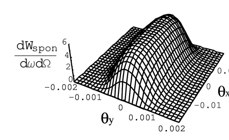
Figure 3: Angular distribution of the spontaneous emission spectrum $\frac{dW_{spon}}{d\omega d\Omega}$ (arbitrary units) versus angles $\theta_{x}$ and $\theta_{y}$ from a single electron with $\gamma_{z}=1000$, $K=p_{x}=20$ for $\omega=0.5\omega_{c}$.

Averaging Eq. (57) over $\theta_{y}$ we obtain

$$\int_{-1}^{1}\frac{dW_{spon}}{d\omega d\Omega}d\theta_{y}=\frac{\sqrt{3}}{2}N_{b}\frac{e^{2}\gamma_{z}}{\pi c}S\left(\frac{2}{3}\frac{\sqrt{2}\eta}{\gamma_{z}^{3/2}\sqrt{p_{x}^{2}-\gamma_{z}^{2}\theta_{x}^{2}}}\right),$$ (60)

where $S\left(x\right)$ is the universal function mentioned in Introduction. Expression (60) can be considered as a radiation power from electron flow in which electrons are evenly distributed over $y$-axis (over direction which is normal to the betatron oscillation plane).

Let us now consider a monoenergetic, axisymmetric electron beam. Radiation spectrum from electron beam with electron distribution function $f\left({\bf p}\right)$ is defined by the relation:

$$\left\langle\frac{dW_{spon}}{d\omega d\Omega}\right\rangle=\int_{0}^{2\pi}\frac{d\phi}{2\pi}\int_{-\infty}^{+\infty}d{\bf p}f\left({\bf p}\right)\frac{dW_{spon}}{d\omega d\Omega}\left({\bf k,p}\right).$$ (61)

Let all electrons have the same longitudinal and transversal energy before interaction and the electron distribution function is

$$f\left({\bf p}\right)=\delta(p_{z}-\gamma_{z})\delta(\sqrt{p_{x}^{2}+p_{y}^{2}}-p_{\bot}).$$ (62)

Then the radiation spectrum from the beam takes a form

$$\left\langle\frac{dW_{spon}}{d\omega d\Omega}\right\rangle=\int_{0}^{2\pi}\frac{d\phi}{2\pi}\frac{dW_{spon}}{d\omega d\Omega}.$$ (63)

In the limit of near-axis radiation $\theta\ll 1/\gamma_{z}$ the radiation spectrum is

$$\left\langle\frac{dW_{spon}}{d\omega d\Omega}\right\rangle\simeq 2N_{b}\frac{3e^{2}}{\pi^{2}c}\left(\frac{\sqrt{2}\eta\gamma_{z}^{3}}{3p_{x}}\right)^{2}K_{2/3}^{2}\left(\frac{\sqrt{2}\eta\gamma_{z}^{3}}{3p_{x}}\right).$$ (64)

In the reverse limit $\theta\gg 1/\gamma_{z}$ the main contribution to Eq. (63) is given by the small values of $\phi\ll 1$ that correspond to the minimum of $q$. The radiation spectrum in this limit is

$$\left\langle\frac{dW_{spon}}{d\omega d\Omega}\right\rangle\simeq\frac{\sqrt{3}}{2}N_{b}\frac{e^{2}\gamma_{z}}{\pi c\theta}S\left(\frac{2}{3}\frac{\sqrt{2}\eta}{\gamma_{z}^{3/2}\sqrt{p_{x}^{2}-\gamma_{z}^{2}\theta^{2}}}\right).$$ (65)

Note that the obtained expression coincides with Eq. (60).

IV Stimulated synchrotron radiation in ion channel

When EM wave of approximately the same frequency as the spontaneous emission is driven through the ion channel simultaneously with the electron beam, a significant exchange of energy between the beam and the wave can occur and can lead to the coherent efficient amplification of the wave energy. This amplification can be explained in terms of the stimulated emission processes which is determined the operation of ICL. Unlike ICL theory ion channel laser , here we will consider regime of strong wiggler ($K\gg 1$) when the emission process is close to synchrotron one. This is the regime of ion-channel synchrotron-radiation laser (ICSRL).

The difference between spontaneous and stimulated emissions is the following. The radiation fields generated by an electron undergoing betatron oscillations has a phase which depends on time of arrival of the electrons at the channel entrance. The fields produced by different electrons in a uniform input beam have a random phase relation to each other and sum up incoherently. This lead to incoherent spontaneous radiation. Contrary to the spontaneous emission, electrons in ion channel can be driven by an external EM wave in synchronous oscillation, the phase of which is no longer random but locked to the phase of the wave. As a result the external wave causes the bunching of the electron beam and more efficient interaction between the beam and the wave. Then the radiation fields of different electrons sum up coherently to each other and to the external wave, leading either to a decrease or to an increase of the power, depending on whether destructive or constructive interference is realized. So the external wave is either absorbed or amplified. In quantum approach the amplification/absorption can be viewed as a transition, forced by the external wave, between the quantum states of the electron in the ion channel with photon absorption/emission. An amplification process of this kind is called a stimulated emission. It is known from laser physics that stimulated emission can be much more efficient and powerful than spontaneous one.

As known in quantum physics haitler there is the relation between the spontaneous and stimulated emission. Using this fact the elementary quantum methods based on the Einstein’s coefficients have been used to study the instability of EM waves in cosmic plasmas astro . Particularly, the synchrotron instability in a cold magnetoactive plasmas has been identified synhrotron instability . The relation between spontaneous and stimulated emission of the electrons in undulators is called Madey’s theorem in the theory of FELs Madey's theorem . It can be considered as extension of Einstein’s coefficient method to the classical limit. Generalized Madey’s theorem book-fel enables us to reduce the problem of ICSRL gain to the problem solved in Sec. III that is the calculation of the power of spontaneous emission in ion channel.

To use Madey’s theorem we should formulate the problem within Hamiltonian approach. An electron motion in an ion channel and in EM wave can be described by a relativistic Hamiltonian

$$H=\sqrt{1+({\bf p}_{\perp}+{\bf A}_{i})^{2}+p_{z}^{2}}+\frac{x^{2}+y^{2}}{4},$$ (66)

where ${\bf A}_{i}$ is the vector potential of the wave with $\theta$ or $\phi$ polarizations ($i=\theta,\phi$):

$$\mathbf{A}_{\theta} = A_{0}\left(\mathbf{e}_{x}\cos\theta\cos\phi+\mathbf{e}_{y}\cos\theta\sin\phi-\mathbf{e}_{z}\sin\theta\right)$$ (67)

$$\times\exp\left[i\eta t-i\eta\left(\mathbf{k}\cdot\mathbf{r}\right)/k\right],$$

$$\mathbf{A}_{\phi}=A_{0}\left(\mathbf{e}_{x}\sin\phi-\mathbf{e}_{y}\cos\phi\right)\exp\left[i\eta t-i\eta\left(\mathbf{k}\cdot\mathbf{r}\right)/k\right].$$ (68)

Hamiltonian (66) is again written in the dimensionless units, normalizing the time to $\omega_{p}^{-1}$, the length to $c/\omega_{p}$, the momentum to $mc$, the vector potential to $mc^{2}/e$. As usual we assume that the time of arrival of the electrons at the channel entrance is random. Assuming that external EM wave is weak we can consider it as perturbation and use the perturbation theory to calculate the work done upon the electron beam by EM wave with $j$-polarization. Then it follows from the generalized Madey’s theorem (see Eq. (5.52) in Ref. book-fel ) that this work per beam electron is

$$\left\langle W_{j}\right\rangle=\frac{1}{2}\frac{\partial\left\langle\gamma_{1,j}^{2}\right\rangle}{\partial\gamma_{0}}+\frac{1}{2}\frac{{\bf k}_{\perp}}{k}\cdot\frac{\partial\left\langle\gamma_{1,j}^{2}\right\rangle}{\partial{\bf p}_{\perp}},$$ (69)

where $\gamma_{1,j}$ is the first-order work done upon a single electron moving along the unperturbed electron trajectory ${\bf r}^{0}\left(t\right)$ by EM wave with $j$-polarization

$$\gamma_{1,j}=\int_{-\infty}^{+\infty}dt\frac{d{\bf r}^{0}\left(t\right)}{dt}\cdot{\bf A}_{i}\left[t,{\bf r}^{0}\left(t\right)\right],$$ (70)

$\gamma_{0}$ and ${\bf p}_{\perp}$ are the electron energy and the transversal momentum of the electron before the interaction. The unperturbed electron trajectory ${\bf r}^{0}(t)$ is determined by Eqs. (22) - (24). Averaging in Eq. (69) implies the averaging over the time of arrival of the electrons at the channel entrance. Mathematical statement of the Madey’s theorem is that the second-order quantity, $\left\langle W_{j}\right\rangle$, is proportional to the average squared first-order quantities, $\gamma_{1,j}$. Therefore Madey’s theorem essentially simplifies calculations in the framework of the perturbation theory. Using instead of variables $\gamma_{0}$ and ${\bf p}_{\perp}$ the initial value of the electron momentum ${\bf p}=({\bf p}_{\perp},p_{z})$, Eq. (69) can be also rewritten in more symmetric form

$$\left\langle W_{j}\right\rangle=\frac{1}{2}\frac{{\bf k}}{k}\cdot\frac{\partial\left\langle\gamma_{1,j}^{2}\right\rangle}{\partial{\bf p}}.$$ (71)

Similar to the FEL theory we introduce the incremental gain of ICSRL as a ratio between a power generated by the electron beam and the incoming EM wave power

$$\Gamma_{j}=\frac{2\lambda^{2}r_{e}n_{b}\left\langle W_{j}\right\rangle}{\pi A_{0}^{2}},$$ (72)

where $n_{b}$ is the density of the electron beam, $r_{e}=mc^{2}/e^{2}$ is the classical electron radius, $\lambda=2\pi c/\omega$ is wavelength of EM wave. It should be noted that to calculate $\left\langle W_{j}\right\rangle$ we consider the given EM wave and do not consider the dynamics of EM wave during the interaction. Hence our calculations is valid for $\Gamma\ll 1$. This regime of interaction is called in the FEL theory as a small-signal small-gain regime book-fel .

It follows from Eqs. (26), (27) and (70) that $\gamma_{1,j}$ is proportional to $I_{j}$. That is the particular case of the general reciprocity relation between the far field of a moving electron and the work done by a plane EM wave on it book-fel . Therefore we can express quantity $\left\langle\gamma_{1,j}^{2}\right\rangle$ through the energy of the spontaneous emission energy radiated per frequency per solid angle

$$\left\langle\gamma_{1,j}^{2}\right\rangle=A_{0}^{2}\left(\frac{e^{2}}{4\pi^{2}c}\frac{\omega^{2}}{\omega_{p}^{2}}\right)^{-1}\frac{dW_{spon,j}}{d\omega d\Omega}.$$ (73)

and can express the gain in term of $\frac{dW_{spon,j}}{d\omega d\Omega}$

$$\Gamma_{j}=\frac{\lambda^{2}r_{e}n_{e}}{\pi}\left(\frac{e^{2}}{4\pi^{2}c}\frac{\omega^{2}}{\omega_{p}^{2}}\right)^{-1}\left(\frac{{\bf k}}{k}\cdot\frac{\partial}{\partial{\bf p}}\right)\frac{dW_{spon,j}}{d\omega d\Omega}.$$ (74)

It has been noted in previous Section that efficient spontaneous emission in direction ${\bf k}$ takes place only at a short moment of time when the electron moment is directed along ${\bf k}$. Therefore we can conclude from Eq. (74) that interaction with EM wave propagating in direction of ${\bf k}$ is only possible at the same moments of time. It was mentioned in Sec. III (see Fig. 3) that the number of the interactions moments is $2N_{b}$. The number of the electron oscillations in EM wave between interaction moments is extremely large: $N_{EMW}\simeq\omega/\omega_{b}\simeq\omega_{c}/\omega_{b}\simeq 3\gamma^{2}K/2$. For example for SLAC experiments $N_{EMW}\simeq 9.2\cdot 10^{9}$. So we can consider the electron phases as random before each interaction moments and, therefore, can consider each interaction moments independently. Using this fact Eq. (74) can be rewritten as follows

$$\Gamma_{j}=2N_{b}\frac{\lambda^{2}r_{e}n_{e}}{\pi}\left(\frac{e^{2}}{4\pi^{2}c}\frac{\omega^{2}}{\omega_{p}^{2}}\right)^{-1}\left(\frac{{\bf k}}{k}\cdot\frac{\partial}{\partial{\bf p}}\right)\left(\frac{dW_{spon,j}}{d\omega d\Omega}\frac{1}{N_{b}}\right).$$ (75)

For simplicity we assume that $p_{y}=0$. To take derivatives in Eq. (75) we should present $\frac{dW_{spon,j}}{d\omega d\Omega}$ as a function of momentum, ${\bf p}$, and use the simplifying assumptions $p_{y}=0$ only after performing differentiation in Eq. (75). This is because the electron motion in the ion channel and in EM wave is no longer plane. Although the unperturbed betatron oscillations is in the plane $y=0$ the action of EM wave leads to the small oscillations along $y$-axis in the first-order of perturbation theory.

It follows from Eqs. (25), (48) and (51) that

$$\left(\frac{e^{2}}{4\pi^{2}c}\frac{\omega^{2}}{\omega_{p}^{2}}\right)^{-1}\frac{dW_{spon,j}}{d\omega d\Omega}\frac{1}{N_{b}}=\frac{2}{\omega_{b}^{2}}\eta^{2}\left|R_{j}\right|^{2}.$$ (76)

Then using Eqs. (32)-(50) we can perform differentiation in Eq. (74). To do it we have to take into account that $\gamma_{z}$, $\omega_{b}$ are the function of $p_{z}$: $\gamma_{z}\left(p_{z}\right)=\sqrt{1+p_{z}^{2}}$, $\omega_{b}\left(p_{z}\right)=$ $1/\sqrt{2\gamma_{z}\left(p_{z}\right)}$. After performing differentiation we can put $p_{y}=0$. Then simplifying the obtained expression with help of MATHEMATICA MATHEMATICA the gain of ICSRL can be derived

$$\Gamma_{\phi} = N_{b}\frac{\sqrt{2}\lambda^{2}r_{e}n_{e}}{9\pi}\frac{\rho^{4}\sin^{2}\phi}{\gamma_{z}^{3}p_{x}}\left[\sin\theta\cos\phi K_{1/3}(q)-\sqrt{\chi}K_{2/3}(q)\right]$$

$$\times\left[\sqrt{\chi}\left(3qT_{0}+\sin\theta\sqrt{\chi}T_{1}\right)K_{1/3}(q)\right.$$

$$-\left.\left(3q\sin\theta\cos\phi T_{0}+\chi^{3/2}T_{2}\right)K_{2/3}(q)\right],$$

$$T_{0} = \sin^{2}\theta\cos^{2}\phi\left[3p_{x}^{3}-8p_{x}^{2}\gamma_{z}\sin\theta\cos\phi-p_{x}\gamma_{z}^{2}\sin^{2}\theta\cos^{2}\phi\right.$$

$$\left.+2\gamma_{z}^{3}\sin^{3}\theta\cos\phi\left(1+2\cos^{2}\phi\right)\right]-3p_{x}^{3},$$

$$T_{1} = 6p_{x}^{3}\cos\phi+2p_{x}^{2}\gamma_{z}\sin\theta\left(3-8\cos^{2}\phi\right)$$

$$-2p_{x}\gamma_{z}^{2}\sin^{2}\theta\cos^{3}\phi-2\gamma_{z}^{3}\sin^{3}\theta\cos^{2}\phi(1-4\cos^{2}\phi),$$

$$T_{2} = 3p_{x}^{3}-8p_{x}^{2}\gamma_{z}\sin\theta\cos\phi-p_{x}\gamma_{z}^{2}\sin^{2}\theta\cos^{2}\phi$$

$$+2\gamma_{z}^{3}\sin^{3}\theta\cos\phi(1+2\cos^{2}\phi),$$

$$\Gamma_{\theta} = N_{b}\frac{\sqrt{2}\lambda^{2}r_{e}n_{e}}{9\pi}\frac{\rho^{4}}{\gamma_{z}^{3}p_{x}}\left[\sin\theta\sin^{2}\phi K_{1/3}(q)+\sqrt{\chi}\cos\phi K_{2/3}(q)\right]$$

$$\times\left[\sqrt{\chi}\left(3q\cos\phi T_{0}+\sin\theta\sqrt{\chi}T_{3}\right)K_{1/3}(q)\right.$$

$$\left.+\left(3q\sin\theta\sin^{2}\phi T_{0}+\chi^{3/2}T_{4}\right)K_{2/3}(q)\right],$$

$$T_{3} = 6p_{x}^{3}-16p_{x}^{2}\gamma_{z}\sin\theta\cos\phi-2p_{x}\gamma_{z}^{2}\sin^{2}\theta\cos^{2}\phi$$

$$+4\gamma_{z}^{3}\sin^{3}\theta\cos\phi\left(1+2\cos^{2}\phi\right),$$

$$T_{4} = 3p_{x}^{3}\cos\phi+2p_{x}^{2}\gamma_{z}\sin\theta\left(3-4\cos^{2}\phi\right)+p_{x}\gamma_{z}^{2}\sin^{2}\theta\cos^{3}\phi$$

$$-4\gamma_{z}^{3}\sin^{3}\theta\cos^{2}\phi\sin^{2}\phi.$$

We have also checked the obtained results by the numerical differentiation for some values of parameters. EM wave can be amplified only if the wave propagates in some small angle to the axis $z$. It is seen from Fig. 4 that there is no amplification of EM wave when the wave propagates along the channel axis.

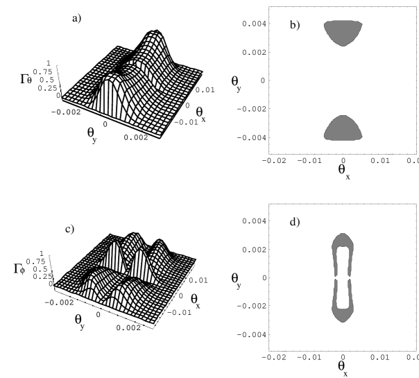
Figure 4: a) $\Gamma_{\theta}$ (arbitrary units), for $\theta$-polarized EM wave with $\omega=\omega_{c}$ versus angles $\theta_{x}$ and $\theta_{y}$ for electrons with $\gamma_{z}=500$, $K=p_{x}=10$. b) The domains of the angles $\theta_{x}$ and $\theta_{y}$ where $\theta$-polarized EM wave with $\omega=\omega_{c}$ is amplified by the electrons $\Gamma_{\theta}<0$, grey region) and where the EM wave is absorbed by the electrons ($\Gamma_{\theta}>0$, white region) for $\gamma_{z}=500$, $K=p_{x}=10$. The angles are given in radians. c) $\Gamma_{\phi}$ (arbitrary units), for $\phi$-polarized EM wave with $\omega=\omega_{c}$ versus angles $\theta_{x}$ and $\theta_{y}$ for electrons with $\gamma_{z}=500$, $K=p_{x}=10$. d) The domains of the angles $\theta_{x}$ and $\theta_{y}$ where $\phi$-polarized EM wave with $\omega=\omega_{c}$ is amplified by the electrons ($\Gamma_{\phi}<0$, grey region) and where the EM wave is absorbed by the electrons ($\Gamma_{\phi}>0$, white region) for $\gamma_{z}=500$, $K=p_{x}=10$. The angles are given in radians.

Eqs. (53) and (52) have been derived under assumption that all electrons have the same momentum before interaction. Now we will consider a monoenergetic, axisymmetric electron beam with electron distribution function given by Eq. (62). ICSRL gain for such electron beam is defined by the relation

$$\left\langle\Gamma_{j}\right\rangle=\int_{0}^{2\pi}\frac{d\phi}{2\pi}\Gamma_{j}\left({\bf p,}\phi\right).$$ (79)

We have performed integration in Eq. (79) numerically. It is seen from Fig. 5 that there is no amplification of EM wave by the beam $\phi$ for given parameters. We are not able to find the wave amplification by the axisymmetric electron beam at least for considered beam parameters.

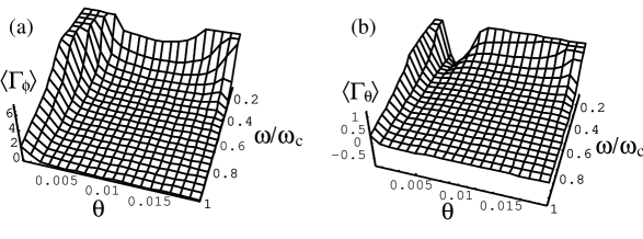
Figure 5: a) $\left\langle\Gamma_{\phi}\right\rangle$ (arbitrary units) for axisymmetric electron beam with $\gamma_{z}=500$, $p_{\perp}=10$ and $\phi$-polarized EM wave versus angle $\theta$ and normolized frequency $\omega/\omega_{c}$. b) $\left\langle\Gamma_{\theta}\right\rangle$ (arbitrary units) for axisymmetric electron beam with $\gamma_{z}=500$, $p_{\perp}=10$ and $\theta$-polarized EM wave versus angle $\theta$ and normolized frequency $\omega/\omega_{c}$.

V Discussion and Conclusions

First we would like to discuss the use a laser-produced ion channel for X-ray generation. As it was mentioned in Introduction an ion channel in plasma can be produced by an electron beam itself. However in this case the plasma density have to be less than beam density. Unfortunately the density of relativistic beam cannot be very high because of technology reasons. This leads to the serious limitation on the gain in radiated power as the power is quadratic in plasma density. Use of high-power laser could overcome this limitation. High-power laser pulse can expel plasma electrons by ponderomotive force and create the ion channel behind the pulse laser channel . Moreover, in strongly nonlinear ”bubble” regime pukhov1 electrons are completely evacuated from the first half-plasma wave excited behind the laser pulse. The ion density in this ”bubble” is higher in many order of magnitude than that in the ion channel formed in the beam - plasma interaction. For example, the ion density in the ”bubble” can be as high as $10^{19}$cm^-3 pukhov1 ; laser channel that is in $10^{5}$ times higher than that in the beam - plasma interaction experiments wang . Therefore the radiated power in laser-produced channel can be in $10^{10}$ times higher than that in the experiments wang for the same number of the betatron oscillations. The ”bubble” moves with group velocity of the laser pulse which is close to the speed of light. Relativistic electron bunch injected into the ”bubble” can propagate inside the ”bubble” over a long distance. Hence, in spite of the small length of the ”bubble” the electrons can oscillate in the ”bubble” a lot of time.

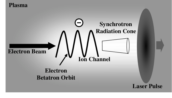
Figure 6: Schematic of the spontaneous emission from external electron beam undergoing betatron oscillations in a laser-produced ion channel.

It should be noted that the self-generated forces of the electron bunch as well as of the relativistic plasma electrons in the column can be neglected because they cancel each other book-beam . The condition to neglect the self-generated forces is $n_{e}\ll n_{i}\gamma^{2}$ that is easily satisfied in modern experiments. The number of the betatron oscillations performed by an electron can be calculated as a ratio of the time during which electron passes through the ”bubble” to the period of the betatron oscillation:

$$N_{b}=\frac{\omega_{p}L}{2\pi\sqrt{2\gamma}(c-v_{gr})},$$ (80)

where $v_{gr}$ is the group velocity of the laser pulse.

Some estimations for parameters in possible and carried out experiments are presented in Table I. To calculate parameters in Table I we assume that $L\simeq 30\mu m$ according to the numerical simulations pukhov1 . The group velocity of the laser pulse in rarefied plasma ($\omega_{L}\gg\omega_{p}$) can be estimated as $v_{gr}/c\simeq 1-\omega_{p}^{2}/\left(2\omega_{L}^{2}\right)$, where $\omega_{L}$ is the laser frequency pukhov1 . Then Eq. (80) can be rewritten as follows

$$N_{b}\simeq 4.7\cdot 10^{10}\frac{1}{\lambda_{L}\left[\mu m\right]\sqrt{\gamma n_{e}\left[cm^{-3}\right]}}\left(\frac{L}{\lambda_{L}}\right),$$ (81)

where $\lambda_{L}$ is the laser wavelength.

Table 1: Parameters of SLAC experiments joshi-review (a); parameters of interaction between 30-GeV electron beam and laser-produced ion channel (b); parameters of interaction between 30-MeV electron beam generated in laser-plasma interaction pukhov1 and laser-produced ion channel (c).

	$r_{0}$	$\gamma$	$n_{i}[cm^{-3}]$	$K$	$\omega_{c}[MeV]$	$N_{b}$	$Q[\frac{MeV}{cm}]$	$N_{ph}$
$a$	$40$	$6\cdot 10^{4}$	$2\cdot 10^{14}$	$17$	$0.12$	$1.5$	$2.5\cdot 10^{-4}$	$0.24$
$b$	$10$	$6\cdot 10^{4}$	$1\cdot 10^{19}$	$1030$	$1889$	$2$	$5.3\cdot 10^{4}$	$21$
$c$	$10$	$6\cdot 10^{2}$	$1\cdot 10^{19}$	$103$	$0.76$	$20$	$5.3$	$21$

It is seen from Table I that use of the laser-produced ion channel can dramatically increase the power of X-ray emission.

In this paper we have studied spontaneous and stimulated emission from electrons undergoing betatron motion in ion channel. We calculate the period of nonlinear betatron oscillations. The method based on the Bessel function expansion is used in Ref. esarey1 to calculate the spectrum of the spontaneous emission in ion channel. However, in synchrotron regime of emission ($K>>1$) the angular distribution of the radiation has been derived in this paper only in the direction which is perpendicular to the electron orbit plane. We extended this result to the arbitrary directions. The generalized Madey’s theorem was used to calculate the electron energy gain of ICSRL. The calculation shows that there is no wave amplification when the EM wave propagates along the channel axis and the amplification takes place only when the wave propagates at some small angle to the channel axis.

Our numerical simulations show that there is no amplification for axisymmetric electron beam at least for considered parameters of the beam. However further analysis is required to justify this conclusion. It may be possible to overcome this difficulty by appropriately tailoring the electron beam, that is, a narrow electron beam could be injected off-axis such that all of the beam electrons execute approximately the same betatron orbit.

To calculate the radiation spectrum and the gain of ICSRL for electron beam, we used a very simple distribution function. Further investigations should include the more realistic electron distribution functions. The gain of ICSRL was calculated in the small-signal small-gain limit. However, it is more interesting for application is to explore large-gain regime of ICSRL that needs further investigations.

References

• (1) E. Esarey et al., IEEE Trans. Plasma Sci. 24 , 252 (1996).
• (2) G. Hairapetian et al., Phys. Rev. Lett. 72, 2403 (1995).
• (3) D. H. Whittum, A. M. Sessler, and J. M. Dawson, Phys. Rev. Lett. 64, 2511 (1990); D. H. Whittum, Phys. Fluids B 4, 730 (1992).
• (4) K. R. Chen and J. M. Dawson, Phys. Rev. Lett. 68, 29 (1992); Phys. Rev. A 45, 4077 (1992).
• (5) C. Joshi, T. Katsouleas, J. M. Dawson, Y. T. Yan, and J. Slater, IEEE J. Quantum Electron. 23, 1571 (1987).
• (6) H. Winick, Sci. Am. 11, 88 (1987).
• (7) S. Wang et al., Phys. Rev. Lett. 88, 135004 (2002).
• (8) C. Joshi et al., Phys. of Plasmas 9, 1845 (2002).
• (9) J. B. Rosenzweig, B. Briezman, T. Katsouleas, and J. J. Su, Phys. Rev. A 44, R6189 (1991).
• (10) J. D. Lawson, The Physics of Charged Particle Beams (Oxford University Press, London, 1988).
• (11) A. Geraci and D. H. Whittum, Phys. Plasmas 7, 2241 (2000).
• (12) C. E. Clayton et al., Phys. Rev. Lett. 88, 154801 (2002).
• (13) J. D. Jackson, Classical Electrodynamics (Wiley, New York, 1975).
• (14) E. Esarey, B. A. Shadwick, P. Catravas, and W. P. Leemans, Phys. Rev. E 6505, 6505 (2002).
• (15) M. H. Key, M. D. Cable, T. E. Cowan et al., Phys. Plasmas 5, 1966 (1998); B. Wharton, C. Brown, B. A. Hammel, S. Hatchett, M. H. Key et al., Phys. Rev. Lett. 81, 822 (1998).
• (16) A. Pukhov and J. Meyer-ter-Vehn, Appl. Phys. B 74, 355 (2002).
• (17) P. Luchini and H. Motz, Undulators and Free-Electron Lasers (Clarendon Press, Oxford, 1990).
• (18) A. Pukhov, Z. M. Sheng, and J. Meyer-ter-Vehn, Phys. Plasmas 6, 2847 (1999).
• (19) I. Yu. Kostyukov, G. Shvets, N. J. Fisch, and J. M. Rax, Phys. Plasmas 9, 636 (2002).
• (20) Handbook of Mathematical Functions, edited by M. Abramowitz and I. A. Stegun (Dover, New York, 1972).
• (21) A. I. Nikishov and V. I. Ritus, Zh. Eksp. Teor. Fiz. 46, 776 (1963) [Sov. Phys. JETP 19, 529 (1964)].
• (22) P. L. Morse and H. Feshbach, Methods of Theoretical Physics (McGraw-Hill Book Company, New York, 1953), Part I, p. 440.
• (23) L. D. Landau, E. M. Lifshits, The Classical Theory of Fields (Pergamon, New York, 1982), 3rd revised English ed., Chap. 73.
• (24) W. Heitler, The Quantum Theory of Radiation (Oxford University Press, London, 1954).
• (25) R. L. Twiss, Australian J. Phys. 2, 564 (1958); V. L. Ginzburg and V. V. Zhelenyakov, Astron. Zh. 35, 694 (1958).
• (26) V. V. Zheleznyakov, Soviet Phys. JETP 24, 381 (1967); P. C. W. Fung, Plasma Phys. 11, 285 (1969).
• (27) J. M. J. Madey, Nuovo Cimento 50B, 64 (1979).
• (28) S. Wolfram, MATHEMATICA (Addison - Wesley, New-York, 1991) 2nd ed.