Statistics for transition of a plasma turbulence with multiple characteristic scales

Abstract

Subcritical transition of an inhomogeneous plasma where turbulences with different characteristic space-time scales coexist is analyzed with methods of statistical physics of turbulences. We derived the development equations of the probability density function (PDF) of the spectrum amplitudes of the fluctuating electro-static potential. By numerically solving the equations, the steady state PDFs were obtained. Although the subcritical transition is observed when the turbulent fluctuations are ignored, the PDF shows that the transition is smeared out by the turbulent fluctuations. It means that the approximation ignoring the turbulent fluctuations employed by traditional transition theories could overestimate the range where hysteresis is observed and statistical analyses are inevitably needed.

I Introduction

Transition phenomena with sudden changes of states are observed in turbulent plasmas. Since these transition phenomena like the L-H transition play crucial roles for magnetic confinement of fusion plasmas, the transition associated with formation of transport barriers is one of the main subjects of high-temperature plasma physics.

Traditional theories for transition of high-temperature plasmas are formulated in terms of averaged physical quantities Itoh and Itoh (1988); Shaing and E. C. Crume (1989). Fluctuations around the averages are ignored and transition phenomena are described deterministically.

However, high-temperature plasmas are strongly non-linear systems with huge number of degrees of freedom and hence their behavior should be chaotic and unpredictable in a deterministic way. In fact, broad distribution of critical values of parameters where transitions occur and intermittent transport called “avalanche phenomena” are observed in recent experiments ITER H-Mode Database Working Group (1994); Politzer (2000); Yoshizawa et al. (2002). Occurrence of these behaviors, which cannot be described only by averaged quantities, are considered due to strong turbulent fluctuations. It is inevitable to describe turbulent plasmas in terms of probability or ensembles like numerical forecast of weather, since the magnitudes of fluctuations around averages are of the same order as that of the averages in turbulent states.

Therefore, transition takes place as a statistical process in the presence of stochastic noise sources induced by turbulence interactions. As a generic feature, transition is expected to occur with a finite probability when a control parameter approaches the critical value.

Statistical theories for plasma turbulence have been developed and the framework to calculate the probability density function (PDF), the transition probability etc. has been made Bowman et al. (1993); Krommes (1996, 1999, 2002); Itoh and Itoh (1999, 2000); Itoh et al. (2002a); Yoshizawa et al. (2002). In the statistical theories, the time-development of the system is described by a set of differential equations with random forces, called the “Langevin equations”. All the information on the statistical properties of the system is obtained by solving the Langevin equation.

The framework has been applied to cases where only one turbulent mode is excited and the turbulence is characterized by one space-time scale Bowman et al. (1993); Krommes (1996, 1999, 2002); Itoh and Itoh (2000); Itoh et al. (2002b); Kawasaki et al. (2002a, b).

However, it is well known that there are many kinds of turbulent fluctuations in high-temperature plasmas and that different characteristic length scales coexist. The importance of interactions between modes with different scale lengths has recently been recognized. For instance, the dynamics of the meso-scale structure of the radial electric field Biglari et al. (1990); Itoh et al. (1999); Terry (2000) is known to cause variation in the dynamics of microscopic fluctuations like in the electric filed domain interface Itoh et al. (1991); Diamond et al. (1997), zonal flow Smolyakov and Diamond (1999) and streamer Drake et al. (1995). Coexistence of multiple scale turbulence has also been investigated by use of the direct numerical simulations Yagi et al. (2002); Kishimoto et al. (2002). Statistical theory on zonal flow dynamics Krommes and Kim (2000) and that of the L-H transition theory has been developed Itoh et al. (2002b).

In the present paper, we apply the statistical theoretic algorithm to a model of high-temperature plasma where two characteristic scales coexist. One is the current diffusive interchange mode (CDIM) micro turbulence Itoh et al. (1999), whose characteristic length scale is of the order of the collisionless skin depth $\delta=c/\omega_{p}$. The other is the ion-temperature gradient (ITG) mode turbulence, whose characteristic wave length is of the order of the ion gyroradius $\rho_{i}$, as an example of the drift wave fluctuations considered to dictate a considerable part of the turbulent transport Horton (1999). Hereafter, we call these two modes “the high wave number mode” and “the low wave number mode” respectively for its simplicity. We assume that the condition $\rho_{i}\gg\delta$ holds. Both turbulences are considered to cause the anomalous transport and hence the coexistence of the high wave number mode and the low wave number mode turbulences and their interplay should be taken into account.

It is known that the subcritical transition occurs in this system, when the pressure-gradient and the radial electric field are changed Itoh and Itoh (2001). However, the turbulent fluctuations are ignored in the analysis. In the present paper, with the statistical theory, we analyze the effect of the turbulent fluctuations on stochastic properties of the transition and show that the fluctuation changes the phase structure of the system completely. More precisely, we show that the transition is smeared out by noises, i.e., the physical quantities changes gradually without clear transition.

The present paper is organized as follows; the statistical theory and the model are formulated in Sec. II. The results of deterministic analyses including occurrence of the subcritical bifurcation are summarized in Sec. III. The Section IV, i.e., the main part of this paper, presents the statistical properties of the system. Summary and discussions are given in Sec. V.

II Theoretical framework and the model

In this section, we briefly review the theoretical framework and the model of turbulent plasmas where two different characteristic scales coexist Itoh and Itoh (2001).

The starting point of the theory is the reduced MHD for the three fields: the electro-static potential, the current and the pressure. The Langevin equation that the statistical theory is based upon is derived as one of model equations which reproduce the two-time correlation functions and the response functions obtained by the renormalization perturbation theory (the direct-interaction approximation) for the reduced MHD Krommes (2002).

The Langevin equation describes time-development of two variables characterizing the system. One is the spectrum amplitude of the electro-static potential for the characteristic wave number $k_{h}$ of the high wave number mode, $x_{h}\equiv k_{h}^{2}\langle\phi^{*}_{k_{h}}\phi_{k_{h}}\rangle/D_{h}^{2}$, and the other is that for the low wave number mode, $x_{l}\equiv k_{l}^{2}\langle\phi^{*}_{k_{l}}\phi_{k_{l}}\rangle/D_{l}^{2}$, whose characteristic wave number is $k_{l}$. Here, $D_{h}$ and $D_{l}$ denote the renormalized transport coefficients for the high wave number mode and the low wave number mode respectively when there is no interactions between two modes. The characteristic time constants for the two modes are defined as

$$\omega_{l}\equiv k_{l}^{2}D_{l},\omega_{h}\equiv k_{h}^{2}D_{h}.$$ (1)

See Itoh and Itoh (2001) for the details of the notation.

The Langevin equation gives the time-development of these two variables as

$$\frac{dx_{l}}{d(\omega_{l}t)}+\frac{1}{2}\left(\frac{\sqrt{x_{h}}}{r}+\sqrt{\frac{x_{h}}{r^{2}}+4x_{l}}-2\right)x_{l}+\frac{1}{2}\left(\frac{\sqrt{x_{h}}}{r}+\sqrt{\frac{x_{h}}{r^{2}}+4x_{l}}\right)x_{l}w_{l}=0,$$ (2)

$$\frac{dx_{h}}{d(\omega_{h}t)}+\left[\sqrt{x_{h}}-\sqrt{1+\frac{\sqrt{x_{l}}}{\sqrt{x_{h}}/r+\sqrt{x_{h}/r^{2}+4x_{l}}}}/(1+pr^{2}x_{l})\right]x_{h}+x_{h}^{3/2}w_{h}+\sqrt{\epsilon}w_{t}=0.$$ (3)

Nonlinear drags and magnitudes of the noises have been evaluated in Itoh and Itoh (2001).

In these equations, the nonlinear terms of the reduced MHD are divided into two parts: One part is coherent with the test field and is renormalized into the deterministic terms, i.e., the second terms. The other is incoherent and is modeled by random forces $w_{h},w_{l}$. Another random force $w_{t}$ denotes the thermal noise and the magnitude of the noise, $\epsilon$, is a small quantity compared to the magnitudes of other noises. Technically, introduction of $\epsilon$ is needed in order to exclude singularity at $x_{h}=0$ of the PDF.

Since $w_{h},w_{l}$ and $w_{t}$ are forces which fluctuates randomly in time, the Langevin equation describes the stochastic time-development of the turbulent fluctuation of the system. For simplicity, we assume that the random forces are Gaussian and white;

$$\langle w(t)w(t^{\prime})\rangle=\delta(t-t^{\prime}).$$ (4)

This system is sustained by the space inhomogeneities, the curvature of the magnetic field $\Omega^{\prime}$, the pressure gradient $dP_{0}/dx$ and the gradient of the radial electric field $dE_{r}/dr$. Here, the shear of the magnetic field is given as the slab configuration: $\mathbf{B}=(0,B_{0}sx,B_{0})$ where $B_{0}(x)=\mbox{const}\times(1+\Omega^{\prime}x+\cdots)$. The pressure is assumed to change in $x-$direction. These driving forces are characterized by the parameter $r$ and $p$ as $r\equiv D_{l}/D_{h}\propto(\Omega^{\prime}dP_{0}/dx)^{-1/2},p\equiv D_{h}^{2}/I_{eff}^{h\leftarrow l}\propto(dE_{r}/dr)^{-6}\Omega^{\prime}dP_{0}/dx$. Here, $I_{eff}^{h\leftarrow l}$ denotes the critical strength of the nonlinear interactions between the low and high wave number modes. The pressure gradient controls the growth rate of the low wave number mode and $\Omega^{\prime}dP_{0}/dx$ excites both the high and low wave number mode turbulences. The gradient of the radial electric field suppresses turbulences Biglari et al. (1990); Itoh et al. (1999); Terry (2000).

We assume that the relation $\rho_{i}\gg\delta$ holds and hence the characteristic length-scales for the two modes are widely separated as

$$k_{h}\gg k_{l}.$$ (5)

The mutual interactions between the low and high wave number modes are asymmetric, since the spatial structure of the low wave number mode is a large-scale inhomogeneity for the high wave number mode. The assertion Eq. (5) also means that the time-scales are widely separated since the time scales are given by Eq. (1);

$$\omega_{h}\gg\omega_{l}.$$ (6)

By analyzing the Langevin equation, Eqs. (2, 3), a number of statistical properties of turbulent plasmas can be derived. For example, the analytical formulae of the rate of change of states of plasmas, the transition rates, were derived. Furthermore, since the renormalized transport coefficients and the random forces have the same origin, i.e., nonlinear interactions in MHD turbulence, relations between the fluctuation levels of turbulence and the transport coefficients like the viscosity and the diffusivity were derived.

III Bifurcation without random forces

With the theoretical framework briefly described in the previous section, we analyze the model of the inhomogeneous plasma with two characteristic scales.

At first, we show the steady state solutions when random forces are ignored, in order to compare to the results with the random forces obtained later. The steady state solutions are obtained by solving the set of nonlinear equations when the random forces are turned off:

$$\left(\frac{\sqrt{x_{h}}}{r}+\sqrt{\frac{x_{h}}{r^{2}}+4x_{l}}-2\right)x_{l}=0,$$ (7)

$$\left[\sqrt{x_{h}}-\sqrt{1+\frac{\sqrt{x_{l}}}{\sqrt{x_{h}}/r+\sqrt{x_{h}/r^{2}+4x_{l}}}}/(1+pr^{2}x_{l})\right]x_{h}=0.$$ (8)

Figure 1: The $r$-dependence of the steady state solutions when no random force. The parameter $p$ is fixed as $p=30$. The solid line represents the low wave number mode $x_{l}$ and the dotted line represents the high wave number mode $x_{h}$. It is seen that the subcritical bifurcation occurs.

Figure 1 shows the $r$-dependence when $p=30$. When $r\leq 0.49\ldots$, the low wave number mode turbulence is suppressed. As $r$ is increased, the system experiences the subcritical transition to the state where the low wave number mode turbulence is excited. When $0.49\ldots<r<1$, there are two stable solutions and it means that the system is bi-stable. From the deterministic point of view, the transition is expected to occur only at the ridge point and the bifurcation point. The qualitative behavior does not depend on the value of $p$ as far as $p>1.9\ldots$.

The phase diagram is shown in Fig. 2. The subcritical bifurcation is observed when the value of the parameter $p$ is larger than $1.9\ldots$. On the other hand, when $p\leq 1.9\ldots$, the bifurcation is supercritical.

Figure 2: The phase diagram when the random forces are turned off. The subcritical bifurcation is observed when $p>1.9\ldots$ and the boundaries of the bi-stable phase are represented with the solid line. When $p\leq 1.9\ldots$, the bifurcation is supercritical and critical values are plotted with the dotted line. The region indicated as “h phase” is the state where the high wave number mode is excited and the region “l phase” is the state where the low wave number mode is excited.

IV The stochastic properties

In the rest of the present paper, we analyze the stochastic properties of the model, Eqs. (2, 3), to investigate the effect of the turbulent fluctuations, i.e., the random forces.

IV.1 The adiabatic approximation and the Fokker-Planck equation

At first, we approximate the Langevin equation Eqs. (2, 3) with making use of the time scale separation between the low and high wave number mode turbulences.

The scale separation, Eq. (6), means that the high wave number mode $x_{h}$ quickly relaxes to the steady state determined by the value of the low wave number mode variable $x_{l}$ which is fixed at the value $x_{l}=x_{l}(t)$ at the time.

We analyze the steady state of the high wave number mode $x_{h}$ when $x_{l}$ is fixed. A state of a stochastic system is described by the probability that a state variable takes a certain value. The time-development of the probability density function (PDF) $P(x_{h},t)$ of $x_{h}$ is determined by Kramers-Moyal expansion applied to the Langevin equation of $x_{h}$, Eq. (3). The Kramers-Moyal expansion is given as

$$\frac{\partial P(x_{h},t)}{\partial t}=-\frac{\partial}{\partial x_{h}}C_{1}(x_{h})P(x_{h},t)+\frac{1}{2}\frac{\partial^{2}}{\partial x_{h}^{2}}C_{2}(x_{h})P(x_{h},t).$$ (9)

The expansion can be truncated at the second order, since the random forces in the Langevin equation are assumed to be Gaussian. Here, the coefficient $C_{n}(x_{h})$ is given by

$$C_{n}(x_{h})\equiv\lim_{\triangle t\rightarrow 0}\frac{1}{\triangle t}\left\langle[x_{h}(t+\triangle t)-x_{h}(t)]^{n}\right\rangle,$$ (10)

where $\langle\cdot\rangle$ denotes the average over the all realizations of the random forces and the average is taken under the condition $x_{h}(t)=x_{h}$. The resulting equation of motion of the probability density function is called the Fokker-Planck equation and is written as

$$\frac{\partial P(x_{h},t)}{\partial(\omega_{h}t)}=\frac{\partial}{\partial x_{h}}\left[\sqrt{x_{h}}-\sqrt{1+\frac{\sqrt{x_{l}}}{\sqrt{x_{h}}/r+\sqrt{x_{h}/r^{2}+4x_{l}}}}/(1+pr^{2}x_{l})\right]$$

$$\times x_{h}P(x_{h},t)+\frac{1}{2}\frac{{\partial}^{2}}{\partial x_{h}^{2}}(x_{h}^{3}+\epsilon)P(x_{h},t).$$ (11)

The steady state solution of Eq. (11) when $x_{l}$ is fixed is shown in Fig. 3. It is seen that the peak of the PDF is relatively narrow and it means that the high wave number mode turbulence spends most of time at the peak value $x_{h}^{*}$. Hence, we can say that it is good approximation to replace $x_{h}$ in the Langevin equation of the low wave number mode with the peak value $x_{h}^{*}$.

Figure 3: The steady state PDF $P(x_{h})$ when $x_{l}$ is fixed at $x_{l}=1$. The peak of the PDF is relatively narrow and the adiabatic approximation that $x_{h}$ is replaced with the peak value of the PDF, $x_{h}^{*}(x_{l})$, is justified. The arrow indicates the location of the peak.

The equation to determine the location of the peak $x_{h}^{*}$ is given by the condition $dP(x_{h}^{*})/dx_{h}^{*}=0$ as

$$\sqrt{1+\frac{\sqrt{x_{l}}}{\sqrt{x_{h}^{*}}/r+\sqrt{x_{h}^{*}/r^{2}+4x_{l}}}}/(1+pr^{2}x_{l})-\frac{3}{2}x_{h}^{*}-\sqrt{x_{h}^{*}}=0.$$ (12)

It is important to note that Eq. (12) is essentially different from Eq. (8) in existence of the second term of Eq. (12), which comes from the random force $x_{h}^{3/2}w_{h}$ of Eq. (3). It implies that the random forces change the steady state of the high wave number mode.

Consequently, the adiabatically approximated Langevin equation for the low wave number mode is given by Eq. (2) where $x_{h}$ is replaced with $x_{h}^{*}$ determined by Eq. (12). The reduced Langevin equation is written as

$$\frac{dx_{l}}{d(\omega_{l}t)}+\frac{1}{2}\left(\frac{\sqrt{x_{h}^{*}}}{r}+\sqrt{\frac{x_{h}^{*}}{r^{2}}+4x_{l}}-2\right)x_{l}+\frac{1}{2}\left(\frac{\sqrt{x_{h}^{*}}}{r}+\sqrt{\frac{x_{h}^{*}}{r^{2}}+4x_{l}}\right)x_{l}w_{l}=0.$$ (13)

The corresponding Fokker-Planck equation, which determines the time-development of the PDF of $x_{l}$, $P(x_{l},t)$, is given by

$$\frac{\partial P(x_{l},t)}{\partial(\omega_{l}t)} = \frac{1}{2}\frac{\partial}{\partial x_{l}}\left(\frac{\sqrt{x_{h}^{*}}}{r}+\sqrt{\frac{x_{h}^{*}}{r^{2}}+4x_{l}}-2\right)x_{l}P(x_{l},t)$$ (14)

$$+\frac{1}{2}\frac{{\partial}^{2}}{\partial x_{l}^{2}}\left[\frac{1}{4}\left(\frac{\sqrt{x_{h}^{*}}}{r}+\sqrt{\frac{x_{h}^{*}}{r^{2}}+4x_{l}}\right)^{2}x_{l}^{2}\right]P(x_{l},t).$$

IV.2 The probability density functions and the effect of the random forces

In this subsection, we investigate properties of the steady state PDF of the low wave number mode, $P(x_{l})$, by numerically solving Eq. (14). Although we will show figures when the parameter $p$ is fixed at $p=30$, qualitative behavior is the same as that for other $p$ values larger than $1.9\ldots$.

At first, we show in Fig. 4 the steady state PDF in the small $r$ region.

Figure 4: The steady state PDF $P(x_{l})$ in the small $r$ region. It shows that the probability that the low wave number mode is suppressed is large and the result is compatible with that of the deterministic analyses given in Fig. 1.

In this region, we have seen that the low wave number mode is suppressed when the turbulent fluctuations are ignored. Figure 4 shows that the probability that the low wave number mode is quiet is large and hence the analysis ignoring random forces is a good approximation in this region.

However, as the value of the parameter $r$ is increased, the characteristics change completely. The steady state PDF when $r>0.49\ldots$ is shown in Fig. 5.

Figure 5: The steady state PDFs of $x_{l}$ when $0.49\ldots<r$. The solid line represents the PDF for $r=0.7$ and the dotted line represents the PDF for $r=1.5$. The wide peak which consists of two small unresolved peaks means that the subcritical transition cannot be observed due to the turbulent fluctuations.

In the region $0.49\ldots<r<1$, we have seen that the subcritical transition occurs and the system is bi-stable if the random forces are ignored. Although there are two peaks in the PDF which are compatible with the previous result without random forces, the valley between the peaks is too shallow to identify the two states. In other words, even if one observes the time-series of $x_{l}(t)$, the value of $x_{l}(t)$ strolls around the two peaks without a sudden change. It means that the bi-stability of the system, i.e., the subcritical transition, is smeared out by the turbulent fluctuations.

The steady state PDF for $r>1$ is also shown in Fig. 5. It is seen that the PDF has a single peak. The single peak is compatible with the result of the deterministic analysis, where only one state exists. However, the peak is wide and hence $x_{l}$ fluctuates widely around the location of the peak. The variance of the fluctuation is as large as the peak value and it means that the fluctuation cannot be ignored. Furthermore, the peak value $0.29\ldots$ obtained when $r=1.5,p=30$ is different from the root of Eqs. (7, 8), which is given as $x_{l}\simeq 0.98$.

In order to see these consequences explicitly, in Fig. 6, we show the comparison of the contour plot of the PDF and the bifurcation diagram obtained by the analysis ignoring the random forces.

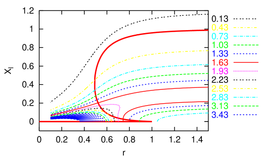
Figure 6: The contour plot of the $r$-dependence of the PDFs. The thin lines represent the contour lines. All the contours larger than $3.43$ are displayed with the same dotted lines. The bifurcation diagram represented with the bold solid line is added for comparison. The location of the region with large probability, mainly denoted with the thin solid lines, is shifted as the value of the parameter $r$ is changed. However, there is no singularity on that.

It is seen that the location of the region which has large probability and mainly denoted with the thin solid lines in Fig. 6 is shifted gradually as the value of the parameter $r$ is changed. Furthermore, the location of the peak of the PDF is far from the result when the random forces are ignored when $r\geq 0.49\ldots$.

Next, in order to investigate the meaning of the average in such a turbulent system, we analyze the tail of the steady state PDF $P(x_{l})$ shown in Fig. 7.

Figure 7: The log-log plot of the tails of the steady state PDFs for different values of $r$. All the tails are well-approximated by the same power-law.

It is shown that the tail of the PDF is well-approximated by the power-law and hence the probability is distributed broadly over large values of the fluctuation. The exponent is about $-0.34$ for the case shown in Fig. 7. It means that the average, i.e., “the center of mass” of the PDF, is shifted in the large $x_{l}$ direction with the long tail and hence the average is not equal to the value that $x_{l}$ takes with large probability. The values that $x_{l}$ takes with large probability are characterized by the peaks of the PDF and are called the most probable values. The difference between the average and the most probable value is shown in Fig. 8.

Figure 8: Comparison of the averages with the most probable values. The averages are indicated with the dashed arrows and the most probable values (the peaks of the PDFs) are indicated with the solid arrows. The difference due to the long tail shown in Fig. 7 means that the average is not equal to the value which $x_{l}$ takes with the largest probability.

Furthermore, hysteresis cannot be captured by observing the average, since the quantity is single-valued from its definition. On the other hand, the most probable values depict the hysteresis as shown in Fig. 9. Although relatively steep variation of the average is observed, the hysteresis can be seen only for the most probable values.

Figure 9: The $r-$dependence of the most probable values (solid lines). The average is also plotted for comparison (a dotted line). Although relatively steep variation of the average is observed, the hysteresis can be seen only for the most probable values.

V Summary and discussion

Finally, we summarize our results and consider their implications. We applied the statistical theory to the model of the inhomogeneous turbulent plasma where two turbulences well-separated in those space-time scales coexist; the “high wave number mode” turbulence (the CDIM micro turbulence) and the “low wave number mode” turbulence (the ITG mode semi-micro turbulence). We derived the development equations of the PDFs of the spectrum amplitudes of the electro-static potential for the characteristic wave numbers. By numerically solving the adiabatically approximated Fokker-Planck equation, the steady state PDFs for the low wave number mode turbulence were obtained. Although the subcritical bifurcation is observed when the turbulent fluctuations are ignored, the shape of the PDF shows that the transition is smeared out by the fluctuations. It means that the approximation ignoring the turbulent fluctuation like the traditional transition theories could overestimate the range of cusp catastrophe.

We also compared the average values with the most probable values and showed that these two characteristic values of stochastic nature are different due to the long power-law tail of the PDF. It means that the average does not mean the value which is expected to realize most probably and hence description of the state of the turbulent systems needs not only the average but also other statistical quantities like the most probable values and the variances.

Consequently, these our results warn that the deterministic description of high-temperature plasmas cannot capture important information of the turbulent systems and the statistical analyses with the Langevin equations and the PDFs are inevitably needed.