Kinetic and Dynamic Delaunay tetrahedralizations in three dimensions

Abstract

We describe the implementation of algorithms to construct and maintain three-dimensional dynamic Delaunay triangulations with kinetic vertices using a three-simplex data structure. The code is capable of constructing the geometric dual, the Voronoi or Dirichlet tessellation. Initially, a given list of points is triangulated. Time evolution of the triangulation is not only governed by kinetic vertices but also by a changing number of vertices. We use three-dimensional simplex flip algorithms, a stochastic visibility walk algorithm for point location and in addition, we propose a new simple method of deleting vertices from an existing three-dimensional Delaunay triangulation while maintaining the Delaunay property. The dual Dirichlet tessellation can be used to solve differential equations on an irregular grid, to define partitions in cell tissue simulations, for collision detection etc.

Pacs: 02.40.S, 02.10.R

In nearly all aspects of science nowadays simulations of discrete objects underlying different interactions play a very important role. Such an interaction for example could be mediated by colliding grains of sand in an hourglass or – more abstract – the neighborhood question of influence regions. One general method to represent possible two-body interactions within a system of $N$ objects is given by a network which can be described by an $N\times N$ adjacency matrix $\nu$, with its matrix elements $\nu_{ij}=\nu_{ji}$ (undirected graph) representing the interaction between the objects $i$ and $j$. However, for most realistic systems the graph defined this way is not practical if one remembers that the typical size of a system of atoms in chemistry can be ${\mathcal{O}}\left(10^{23}\right)$, the human body consists of ${\mathcal{O}}\left(10^{18}\right)$ cells and even simple systems such as a grain-filled hourglass contain ${\mathcal{O}}\left(10^{3}\right)$ constituents. Even some reasonable fraction of such systems would be far too complex to be simulated by adjacency matrices. However, in most systems in reality the interactions at work have only a limited range. Physical contact forces such as adhesion for example, can only be mediated between next neighbors. In such systems the adjacency matrix elements $\nu_{ij}$ would vanish for all distant constituents and therefore a more efficient description can be given by a sparse graph, where the adjacency relations between objects moving in their parameter space can be updated using rather simple methods. In some systems – such as solids crystallizing in a lattice configuration – the neighborship are uniform and therefore a priori known. This can be effectively exploited if one considers all deviations from a lattice configuration as small perturbations. But also rather heterogenous systems can be modeled by lattice methods, e.g. the method of cellular automata [1] has been used to model cell tissues [2, 3]. Note however, that several adaptations have to be performed in order to account to the different nature of next-neighborship in these systems. In the realistic system of cells in a human tissue for example, the number of next neighbors per cell is neither constant over the cell ensemble nor are the interaction forces. To make things worse, all these parameters become time dependent for dynamic systems. The same holds true in the framework of collision detection.

In this article it is our aim to describe our implementation of a code generating three-dimensional dynamic (supporting insertion and deletion) and kinetic (supporting point movements) Delaunay triangulations. Delaunay triangulations and their geometric dual – the Voronoi tessellation – have been demonstrated before to be suitable tools to model cell tissues [4, 5, 6]. However, these considerations have been restricted to the two-dimensional case. In three-dimensional space kinetic (but not fully dynamic) Delaunay triangulations have been applied e.g. in the framework of collision detection amongst spherical grains [7].

The generation of Delaunay triangulations is a well-covered topic, for a review see e.g. [8, 9, 10]. Such triangulations are widely used for grid generation in finite element calculations and surface generation for image analysis [11]. Since the Delaunay triangulation in general tries to avoid flat simplices, it also produces a good quality mesh for the solution of differential equations [12, 13]. In dimensions higher than two however, the situation is much more complicated. For example, three-dimensional triangulations of the same number of points may have different numbers of tetrahedra [8]. This can be compensated by using more dynamic data structures that allow for a varying number of simplices such as lists. A more serious problem however, is posed by the fact, that a two-dimensional polygon can always be triangulated, whereas a three-dimensional non-convex polyhedron may not admit a decomposition in tetrahedra without using artificial (Steiner) points [14, 15]. These differences result in the important consequence that not all algorithms can be generalized in a straightforward way from two-dimensional Delaunay triangulations. The maintenance of the triangulation in the case of dynamic (moving) vertices now requires a data structure capable of handling a varying number of simplices in time. Another important problem is the deletion of vertices from a Delaunay triangulation which is simple in two dimensions [16, 17] but transforms into a nontrivial problem in higher dimensions [18], because in three dimensions there may exist non-convex polyhedra (e.g. Schönhardt’s polyhedron [14]) that cannot be tetrahedralized [19].
We have implemented algorithms for both adding and deleting vertices to a three-dimensional Delaunay triangulation that are incremental in the sense that they transform a Delaunay triangulation with $n$ vertices into a Delaunay triangulation with $(n+1)$ or $(n-1)$ vertices, respectively. In addition, we have implemented flip algorithms [7, 20, 21] to maintain the Delaunay-property of the triangulation in the case of kinetic vertices. These ingredients together allow to provide a code for dynamic three-dimensional Delaunay triangulations with kinetic vertices. Such a code is suitable for the construction and maintenance of proximity structures for moving objects, e.g. cell tissue simulations, where cell proliferation, cell death, and cell movement are essential elements that have not been covered by Delaunay triangulations in three dimensions before. Since for many neighborhood interaction forces (especially in cell tissues), the contact surfaces and volumes of the dual Dirichlet tessellation is of importance, we have also implemented algorithms to compute these values from a given Delaunay triangulation.

This article is organized as follows:
In section 1 we briefly review the concept of the Delaunay triangulation by addressing the basic conventions in 1.1, the elementary topological transformations in a triangulation in 1.2, defining the Delaunay criterion in 1.3 and considering the geometric dual in 1.4 as well as the more technical volume and surface calculation of Voronoi cells in 1.5. In section 2 we describe the actual implementation of the algorithms by describing the used data structure in 2.1, an incremental insertion algorithm in 2.2, a stochastic visibility walk algorithm in 2.3, the used flip algorithms in 2.4, and close with a description of an algorithm for incremental vertex deletion in 2.5. In section 3 we analyze performances of the incremental insertion algorithm in 3.1, the incremental deletion algorithm in 3.2, the transformation of slightly perturbed Delaunay triangulations into Delaunay triangulations in 3.3, and finally consider the performance of a combination of all processes in 3.4. Robustness ist also briefly addressed. We will close with a summary in section 4.

1 The Delaunay Triangulation

1.1 Conventions

For the sake of clarity, the illustrations in this article will be two-dimensional, unless noted otherwise. Following the notation in the literature [20, 21] we denote by the term vertex a position in three-dimensional space. By an $n$-simplex in ${\mathbb{R}}^{d}$ ($n\leq d$) we understand the convex hull of a set $T$ of $n+1$ affinely independent vertices, which reduces in the three-dimensional case to tetrahedra (3-simplices), triangles (2-simplices), edges (1-simplices) and vertices (0-simplices). Every $n$-simplex has a uniquely defined $n$-circumsphere. Recall that a tetrahedron is bound by four triangles, six edges and four points in three dimensions. These $(n\leq d)$-simplices $\sigma_{U}$ – formed by the convex hull of a subset $U\subseteq T$ – are also called faces of $T$. Since we will work in three dimensions, we will shortly denote 3-simplices by the term simplex. A collection of these simplices $\mathcal{K}$ is called a simplicial complex if:

• The faces of every simplex in $\mathcal{K}$ are also in $\mathcal{K}$

• If $\sigma_{T}\in\mathcal{K}$ and $\sigma_{T^{\prime}}\in\mathcal{K}$, then $\sigma_{T}\cap\sigma_{T^{\prime}}=\sigma_{T\cap T^{\prime}}$.
  (the intersection of two simplices is at most a face of both, the simplices are ’disjoint’)

In numerical calculations with kinetic vertices the above criterion can be destroyed: A vertex might move inside another simplex thus yielding two $n$-simplices whose intersection is again an $n$-simplex. We will refer to this situation as an invalid triangulation. To be more exact, a triangulation is defined as follows. If $S$ is a finite set of points in ${\mathbb{R}}^{d}$, then a simplicial complex $\mathcal{K}$ is called a triangulation of $S$ if

• each vertex of $\mathcal{K}$ is in $S$

• the underlying space of $\mathcal{K}$ is $conv(S)$

By the degree of a vertex in a triangulation we will denote the number of simplices in the triangulation containing the vertex as endpoints. Furthermore, we will use the terms tetrahedralization and triangulation in three dimensions synonymously, unless noted otherwise.

1.2 Elementary Topological Transformations

To an existing triangulation in ${\mathbb{R}}^{3}$ several topological transformations can be applied. We will briefly remind the main ideas. For a more detailed discussion see e.g.  [20, 22]. The discussion basically relies on Radon’s theorem (see e.g. [15, 20]):

Let $X$ be a set of $d+2$ points in ${\mathbb{R}}^{d}$. Then a partition $X=X_{1}\cup X_{2}$ with $X_{1}\cap X_{2}=\emptyset$ exists such that $conv(X_{1})\cup conv(X_{2})\neq\emptyset$.
If $X$ is in general position – meaning that every subset of $X$ with at most $d+1$ elements is affinely independent – then this partition is also unique. In our case this simply means that [10, 21]

• no four points lie on a common plane

• no five points lie on a common sphere

Figure 1 illustrates the idea of Radon’s theorem in three dimensions.

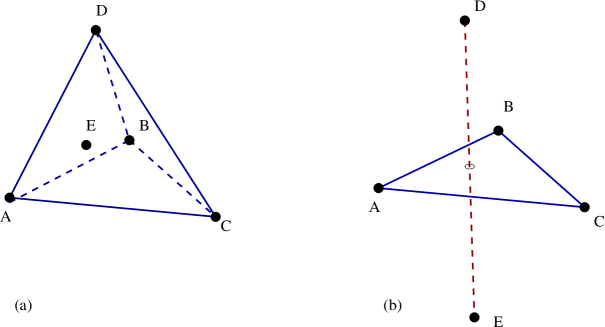
Figure 1: Illustration of the Radon partition in three dimensions. There are two possible constellations of the 5 points A, B, C, D, E in three dimensions. In (a) the point E lies within the simplex formed by (A, B, C, D), whereas in (b) none of the vertices lies within the simplex formed by the other ones.

From the Radon partition in ${\mathbb{R}}^{3}$ one finds that there exist four possible flips in three dimensions, two for every partition in figure 1. For the case of figure 1a the two possible flips are shown in figure 2.

Figure 2: Three-dimensional illustration of the addition or deletion of a vertex E. In the left picture (a) one has exactly four simplices: (A, B, C, E), (A, B, D, E), (A, C, D, E), (B, C, D, E), whereas in the right picture (b) the vertex E lies within the simplex (A, B, C, D). The edges that can principally not be seen from the outside are drawn dashed. Switching between the two configuration corresponds to adding ($1\to 4$) the vertex E to an existing triangulation or deleting it ($4\to 1$), respectively. Note that for these operations to be possible, the point E must lie within the simplex (A, B, C, D).

The flip changing the triangulation from $1$ to $4$ simplices corresponds to adding a vertex to an existing triangulation. Note however, that in practice the inverse transformation may not always be applicable, since the configuration of one vertex ($E$ in figure 2) being the endpoint of exactly four simplices is rarely ever present in a triangulation. This fact – in combination with the existence of non-tetrahedralizable polyhedra in three dimensions – complicates the deletion of vertices from triangulations [18].

The second partition in figure 1b following from Radon’s theorem requires a more careful evaluation, see figure 3.

Figure 3: Three-dimensional illustration of the possible triangulations of five points. In (a) there are two simplices: (A, B, C, D), (A, B, C, E), sharing the common triangle (A, B, C), whereas the right picture (b) consists of three simplices (A, B, D, E), (B, C, D, E), (C, A, D, E). The simplices have been taken apart for clarity and the dotted lines have been drawn to connect the identical points. Invisible Edges have been drawn with dashed lines. Note that the flips can only be performed, if the polyhedron (A, B, C, D, E) is convex, since otherwise the flips will result in overlaps with additional neighboring simplices (not shown here).

The flips $2\to 3$ (and $3\to 2$) can only be performed if the polyhedron formed by the five points in ${\mathbb{R}}^{3}$ is convex, otherwise the operation would yield overlapping simplices in the triangulation. The convexity of $A,B,C,D,E$ in figure 3 can be tested by checking if for every edge $A,B$ and $B,C$ and $C,A$ there exists a hyperplane which has the remaining three points ($D,E,A/B/C$) on the same side [20, 21, 23].

1.3 The Delaunay Criterion

Every tetrahedron in ${\mathbb{R}}^{3}$ has a uniquely defined circumsphere, if the four vertices do not lie on a common plane (i.e. if the tetrahedron is not flat). The Delaunay triangulation is a triangulation where all the simplices satisfy the Empty-Circumsphere-Criterion: No vertex of the triangulation may lie inside the circumspheres of the triangulation simplices. Thus, the Delaunay triangulation is uniquely defined if the vertices are in general position, i.e. if no five vertices must lie on a common sphere and no four vertices may lie on a common plane [10].

The simplest method to determine, whether a vertex $V$ lies outside or inside the circumsphere of a simplex $(A,B,C,D)$ is to solve the associated four sphere equations. However, this problem can be solved more efficiently by adding one more dimension [7, 15, 21].

Suppose we would like to know whether the vertex $E$ lies in- or outside the circumsphere of the simplex $(A,B,C,D)$, which we will – without loss of generality – assume to be positively oriented. Then one can proceed as follows (e.g. [24]): Project the coordinates in ${\mathbb{R}}^{3}$ onto a paraboloid in ${\mathbb{R}}^{4}$ via

$$A=(A_{x},A_{y},A_{z})\to A^{+}=(A_{x},A_{y},A_{z},A_{x}^{2}+A_{y}^{2}+A_{z}^{2})\,.$$ (1)

The four points $A^{+},B^{+},C^{+},D^{+}$ define a hyperplane in ${\mathbb{R}}^{4}$. If $E$ is within the circumsphere of $(A,B,C,D)$, then $E^{+}$ will be below this hyperplane in ${\mathbb{R}}^{4}$ and above otherwise. Consequently, the in-circumsphere-criterion in ${\mathbb{R}}^{3}$ reduces to a simple orientation computation in ${\mathbb{R}}^{4}$, i.e. by virtue of this lifting transformation one finds [7]

$${\rm in\_circumsphere}((A,B,C,D),E)$$ (7)

$$= {\rm oriented}(A^{+},B^{+},C^{+},D^{+},E^{+})$$

$$= {\rm sign}\left|\begin{tabular}[]{ccccc}$A_{x}$&$A_{y}$&$A_{z}$&$A_{x}^{2}+A_{y}^{2}+A_{z}^{2}$&$1$\\ $B_{x}$&$B_{y}$&$B_{z}$&$B_{x}^{2}+B_{y}^{2}+B_{z}^{2}$&$1$\\ $C_{x}$&$C_{y}$&$C_{z}$&$C_{x}^{2}+C_{y}^{2}+C_{z}^{2}$&$1$\\ $D_{x}$&$D_{y}$&$D_{z}$&$D_{x}^{2}+D_{y}^{2}+D_{z}^{2}$&$1$\\ $E_{x}$&$E_{y}$&$E_{z}$&$E_{x}^{2}+E_{y}^{2}+E_{z}^{2}$&$1$\end{tabular}\right|$$

$$= {\rm sign}\left|\begin{tabular}[]{cccc}$A_{x}-E_{x}$&$A_{y}-E_{y}$&$A_{z}-E_{z}$&$(A_{x}^{2}+A_{y}^{2}+A_{z}^{2})-(E_{x}^{2}+E_{y}^{2}+E_{z}^{2})$\\ $B_{x}-E_{x}$&$B_{y}-E_{y}$&$B_{z}-E_{z}$&$(B_{x}^{2}+B_{y}^{2}+B_{z}^{2})-(E_{x}^{2}+E_{y}^{2}+E_{z}^{2})$\\ $C_{x}-E_{x}$&$C_{y}-E_{y}$&$C_{z}-E_{z}$&$(C_{x}^{2}+C_{y}^{2}+C_{z}^{2})-(E_{x}^{2}+E_{y}^{2}+E_{z}^{2})$\\ $D_{x}-E_{x}$&$D_{y}-E_{y}$&$D_{z}-E_{z}$&$(D_{x}^{2}+D_{y}^{2}+D_{z}^{2})-(E_{x}^{2}+E_{y}^{2}+E_{z}^{2})$\end{tabular}\right|\,,$$ (12)

where a positive sign is to be taken as an affirmative answer.

Several algorithms have been developed for the construction of static triangulations [15, 25] as well as for the maintenance of kinetic triangulations [7, 22], some of which will be discussed in section 2.

1.4 The Geometric Dual: Voronoi Tessellation

The most general Voronoi tessellation (sometimes also called Dirichlet tessellation) of a set of generators $\{c_{i}\}$ in ${\mathbb{R}}^{d}$ is defined as a partition of space into regions $V_{i}$:

$$V_{i} = \{x\in\mathbb{R}^{n}\;:\;\mathcal{P}(x,c_{i})\leq\mathcal{P}(x,c_{j})\qquad\forall j\neq i\}\,,$$ (13)

where $\mathcal{P}(x,c_{i})$ can be an arbitrary function, which reduces in the standard case of the simple Voronoi tessellation to the normal euclidian distance ${\mathcal{P}}(x,c_{i})=\left|x-c_{i}\right|$. In other words, the Voronoi cell around the generator $c_{i}$ contains all points in ${\mathbb{R}}^{d}$ that are closer to $c_{i}$ than to any other generator $c_{j}$. Note that this partition is – unlike the Delaunay triangulation – uniquely defined also for point sets that do not fulfill the general position assumption. Voronoi tessellations have many interesting applications in practice – for a survey see e.g. [8] – since they do describe influence regions.

In 2 dimensions Voronoi cells are convex polygons completely covering the plane, see e.g. figure 4. This finding generalizes to arbitrary dimensions: The boundaries between two $d$-dimensional Voronoi regions $V_{i}$ and $V_{j}$ as defined in (13) reduce to the equation for a $d-1$ hyperplane. Therefore per definition the Voronoi cells around generators $Z_{i}$ situated on the convex hull of the point set $Z=\{Z_{1},Z_{2},\ldots,Z_{n}\}$ will extend to infinity and thus will have an infinite volume.

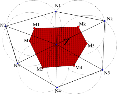
Figure 4: Two-dimensional Voronoi cell around a generator $Z$, which is surrounded by other generators $N_{i}$. All points within the shaded region are closer to the generator Z than to any other generator. The corners of the Voronoi cell polygons $M_{i}$ are the centers of the circumcircles (drawn with dotted lines) of the Delaunay triangulation (solid lines) of the generator set.

Voronoi tessellations can be constructed like the well-known Wigner-Seitz cell in solid state physics [26], but fortunately there are much more efficient ways to construct the Voronoi tessellation. In this work, we will exploit the geometric duality with the Delaunay triangulation: In any dimension, the corners of the Voronoi polyhedra are the centers of the circumspheres of the $n$-simplices contained in the Delaunay triangulation of the Voronoi generators, see figure 4.

The introduction of influence regions also enables the definition of proximity between vertices: We understand two vertices to be direct neighbors (in the sense that their influence regions touch) if they share a common face in their Voronoi diagram or – equivalently – if they are direct neighbors in the dual Delaunay triangulation, see figure 4.

The concept of the Voronoi cell can easily be extended towards generators with a varying strength, the weighted Voronoi tessellation [8]. In such extensions, every generator is assigned a weight, i.e. the functions $\mathcal{P}(x,c_{i})$ in (13) are then given by a function describing the influence strength of the generator $i$ at $c_{i}$ on $x$. Obviously, the weighted Dirichlet regions can – in contrast to the standard unweighted case – be empty, e.g. if a vertex with a weak influence is surrounded by strong vertices. Among many possible choices for weight functions [8, 27] we will explicitly mention here the case of power-weighted Voronoi diagrams, also often called the Laguerre complex [7, 22]. It is obtained by assigning a weight $\omega_{i}\in\mathbb{R}$ to every generator $c_{i}$, i.e. by using $\mathcal{P}(x,c_{i})\to\mathcal{P}(x,c_{i},\omega_{i})=(c_{i}-x)^{2}-\omega_{i}^{2}$ in (13). In the power-weighted case one can still show that in three dimensions the Laguerre cells are convex polyhedra, whose corners can be obtained from the weighted centers of the corresponding weighted Delaunay triangulation tetrahedra – where the empty circumsphere criterion is simply replaced by its weighted counterpart. Therefore, the Laguerre tessellation or its geometric dual – the weighted Delaunay triangulation – is suitable for collision detection between differently sized spheres. We would like to stress that the algorithms in this article can be generalized to the power-weighted case in a straightforward way.

1.5 Voronoi surfaces and volumes

Within the framework of growth models [22], tissue simulations [5, 6] and the solution of partial differential equations on irregular grids [12, 13], not only the neighborship relations in the Delaunay triangulation but also the corresponding Voronoi cell volumes as well as the contact surface between two Voronoi cells may become important. Obviously, to the surface of a Voronoi cell around a vertex $Z$ every incident simplex $\sigma$ with $Z\in\sigma$ contributes, see figure 4. In two dimensions every triangle $(Z,N_{i},N_{i+1})$ contributes two surfaces, spanned by the half distances between the vertices $A=1/2(N_{i}-Z)$ and $B=1/2(N_{i+1}-Z)$, and the center of the circumcircle of $R=COC(Z,N_{i},N_{i+1})-Z$. If $(A,B)$ are positively oriented (which we will further on assume without loss of generality), then the oriented 2-volume contribution of the simplex $(Z,N_{i},N_{i+1})$ to the Voronoi cell volume of the vertex $Z$ is given by

$$V_{Z}=\frac{1}{2}\left(\left|\begin{tabular}[]{cc}$A_{x}$&$R_{x}$\\ $A_{y}$&$R_{y}$\end{tabular}\right|+\left|\begin{tabular}[]{cc}$R_{x}$&$B_{x}$\\ $R_{y}$&$B_{y}$\end{tabular}\right|\right)\,,$$ (18)

see also figure 5 for illustration. Obviously, the sum of the three volumes has to equal the total simplex volume $V_{Z}+V_{N_{i}}+V_{N_{i+1}}=V_{S}$ . One can show algebraically, that this identity holds true for any $R$, i.e. also in the interesting case where $R$ being the center of the circumcircle lies outside the triangle as in figure 5. In this case one of the two area contributions in (18) will be negative. Now when considering figure 5 it becomes clear that by adding the oriented volume contributions of all simplices containing the vertex $Z$ one obtains the correct volume for the Voronoi cell around $Z$.

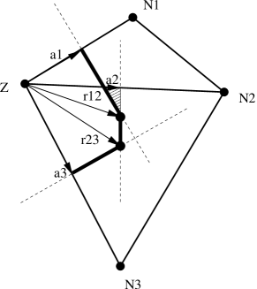
Figure 5: Volume (area) computation of a two-dimensional Voronoi cell around the generator $Z$. Here for clarity only two simplices are shown. The first simplex $(Z,N_{1},N_{2})$ contributes the positive area spanned by $(a_{1},r_{12})$ and the negative area spanned by $(r_{12},a_{2})$. The second contribution is negative because the center of the circumcircle of $(Z,N_{1},N_{2})$ is outside the simplex. Most of the negative volume contribution is thus canceled – up to a small part (hatched region) situated outside the Voronoi cell boundary (thick lines). However, when considering the next simplex $(Z,N_{2},N_{3})$ the positive contribution spanned by $(a_{2},r_{23})$ cancels with this remaining negative contribution from the first simplex. The last contribution comes from $(r_{23},a_{3})$ and is again positive.

This finding generalizes to three-dimensional volume computation, and the three-dimensional contact surface contribution is in fact nothing but a two-dimensional volume computation, since the contact surfaces between two Voronoi polyhedra are plane polygons.

The algorithm leads to a wrong Voronoi cell volume at the boundary, where the Voronoi cells are per definition infinite. However, if the centers of the circumspheres of the simplices at the boundary do not lie outside the convex hull of the triangulation, then the volume summation yields the part of the Voronoi cells which is inside the convex hull. This is desirable for some configurations, such as the solution of partial differential equations [13].

The numerical complexity of the volume computation is linear with the number of simplices surrounding the vertex, whereas the complexity of contact surface calculation between two generators grows linear with the number of simplices containing both generators as endpoints. The algorithm can be checked by using that the sum over all Voronoi cell volumes computed this way has to equal the sum of the simplex volumes in the dual Delaunay triangulation.

2 Algorithms and Implementation

2.1 The Data Structure

As has already been mentioned in the introduction, three-dimensional Delaunay triangulations are much more complicated than in two dimensions. The first difference is that the number of triangulation simplices may vary for a constant number of mobile vertices. Our triangulation basically consists of two data structures:

• a list of the vertices in the triangulation

• a list of connected 3-simplices (tetrahedra) contained in the triangulation

Both structures are organized in a list to enable for the kinetic movement, insertion, and deletion of vertices and the corresponding dynamic update of the simplex list.

A vertex consists of the $x$, $y$ and $z$ coordinates, a weight (which will be assumed to be equal for all points throughout this article) and – to compute the Voronoi cell data efficiently – a vector of all incident tetrahedra. A simplex consists of four pointers on vertices and of four pointers on the neighboring simplices. The latter is required by the fact that we perform a walk in the triangulation (see section 2.3).

The construction of the Delaunay triangulation basically relies on two basic predicates: The determination whether two points lie on the same side of a plane defined by three others and the question whether a point lies in- or outside the circumsphere circumscribing the simplex of four others (enforcement of the Delaunay criterion). By using these two simple predicates the whole triangulation can be built up.

2.2 Incremental Insertion Algorithms

Unfortunately in Delaunay triangulations the insertion of one new vertex can change the whole triangulation, but this only holds true for some extreme vertex configurations, for some examples see [8]. In practice, the effect of adding a new vertex to a Delaunay triangulation will nearly always be local. Anyhow, the algorithms we describe here can of course also cope with these worst case scenarios.

So let us assume we have a valid Delaunay triangulation with $n$ vertices. Let us furthermore assume that the new vertex lies within the convex hull of the $n$ vertices. Then the updated Delaunay triangulation can be constructed as follows (see figure 6):

• Identify all invalid simplices in the triangulation, i.e. all those containing the new vertex within their circumsphere.

• Collect the external facets of the invalid simplices. (Those are the triangles facing valid simplices.)

• Replace the invalid simplices by new ones formed via combining the external facets with the new vertex.

Sometimes this incremental algorithm is also called Bowyer-Watson Algorithm [28, 29]. Once all the invalid simplices have been found, its computational cost is very low (linear with the total number of invalid simplices). At first it actually suffices to find the one simplex which contains the new vertex within its convex hull – the remaining simplices can be found by iteratively checking all neighbors for invalidity, see also figure 6.

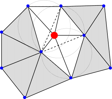
Figure 6: In this example, a new vertex (large point) is inserted into an existing triangulation (not all simplices are shown). Most of the simplices remain valid (shaded region), but 3 simplices (dashed lines) contain the new vertex within their circumspheres (dotted lines). These are replaced by 5 new simplices (solid lines) formed by the new vertex and the external facets (lines in two dimensions). The resulting triangulation fulfills the Delaunay criterion.

The result of this procedure is a Delaunay triangulation with $n+1$ vertices.

The algorithm shown in figure 6 is only slightly different than the Green-Sibson Algorithm [28], which needs the simplex containing the new vertex as an input. Then the elementary topological transformation $1\to 4$ is performed with this simplex and the resulting (Delaunay-invalid) triangulation is transformed to a Delaunay triangulation by performing $2\to 3$ and $3\to 2$ flips until all simplices fulfill the Delaunay property.

Note that for weighted triangulations the simplex containing the new vertex within its convex hull is not necessarily invalid, since the weighted circumsphere does not generally contain the complete simplex. This corresponds to the case of an empty Laguerre cell – the vertex therefore has to be rejected.

The initial triangulation can be given by an artificial large simplex which contains all the data to be triangulated within its convex hull. Therefore, the convex hull of the points to be triangulated is contained within the artificial simplex and is not reproduced by the triangulation. However, in the framework of kinetic proximity structures this has the advantage that one does not have the problem of maintaining the convex hull of moving points, since the artificial simplex does not move. The initial simplex must therefore be large enough to contain the data within its insphere throughout the full time evolution of the simulation. One choice for such an initial simplex is a $\rm{CH}_{4}$ configuration.

2.3 Location of Simplices

The incremental insertion algorithm requires a first initial simplex containing the new vertex. Many all implementations of Delaunay triangulations perform a walk in the triangulation, for an overview of different walking strategies see e.g. [30]. Note that points can also be located by using the history the triangulation has been constructed (e.g. the so-called Delaunay tree [28] or history dag [31]). However, we are aiming at kinetic triangulations, where the length of a history stack could not be controlled.

Here we will use a stochastic visibility walk [30] to locate a simplex containing a point. Starting with an arbitrary initial simplex $A$ and a new vertex $v$ to be inserted in the triangulation, in the normal visibility walk one of the four neighbor simplices of $A$ is chosen using the following criterion:

• For all four vertices $a_{i=1,2,3,4}$ of the simplex $A$ check with the new vertex $v$:
  Are the vertices $a_{i}$ and $v$ on different sides of the plane defined by the other three vertices $a_{j\neq i}$, i.e. is it visible from the plane defined by the $a_{j\neq i}$?
  yes : $\Longrightarrow$ Jump to the simplex opposite to $a_{i}$.

• If no neighbor simplex is found, the vertex $v$ is contained within the simplex $A$ and the destination is thus reached.

Obviously, the algorithm can take different pathways (see figure 7) since there may be more than one neighbor fulfilling this criterion. Note also that due to numerical errors the normal visibility walk may loop when triangulating regular lattices (such as cubic, …) that violate the general position assumption. Such situations can be easily avoided by using the stochastic visibility walk, where the order of the vertices to be checked is randomized. Such a stochastic visibility walk terminates with unit probability [30].

The complexity is directly proportional to the length of the path to be walked – measured in units of traversed simplices. For $n$ uniformly distributed vertices for example, the average total number of simplices will grow linearly ($n$) with the number of vertices, whereas the average distance between two arbitrarily selected simplices will grow like $n^{1/3}$. Once the invalid simplex has been found, the average remaining complexity for the incremental insertion will be in average constant (in $n$). Therefore one would expect the overall theoretical complexity to behave like $\alpha n^{4/3}+\beta n$ for uniformly distributed points and in higher dimensions $d$ as $\alpha n^{1+1/d}+\beta n$, see also [32].

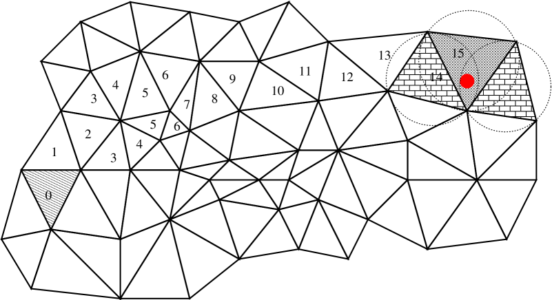
Figure 7: Two-dimensional illustration of the hopping algorithm in a triangulation (not all simplices are shown). Starting from the hatched initial simplex $0$ the algorithm finds a way towards the invalid simplex $15$ (cross-hatched) that contains the new vertex (large point). The computational time necessary for the walk algorithm is proportional to the number of traversed simplices.

Obviously, the algorithm heavily depends on a good choice of the starting simplex. The method could therefore be improved by checking whether the new vertices lies within a certain subregion which means preprocessing, or it can be speeded up by initially using larger step sizes, e.g. by using several triangulations of subsets of vertices [25]. Alternatively, one can choose the closest vertex out of a random subset of the triangulation to find a good starting simplex [33, 34]. In some sense these two methods are similar, since finding a close vertex is nothing but finding the Voronoi-cell the point is situated in. The second method however does not require the maintenance of an additional triangulation in the case of kinetic vertices.

In many practical simulations, some neighborship relations may already be known when building the initial triangulation. Our implementation of the incremental algorithm therefore expects the vertices to be included in some order, such that successive vertices are also very close to each other in the final triangulation and therefore chooses the starting simplex in the walk algorithm as being the last simplex created if no other guess is given. Note that for processes as cell proliferation, the situation is even better: New cells can be created by cell division which corresponds to the insertion of a new vertex close to an existing one. Consequently, one always has a perfect guess for the starting simplex in these cases.

2.4 Updating the triangulation

In three-dimensional kinetic triangulations where the vertices are moving and neighborship relations can change, one has to deal with a changing number of simplices. Once deletion and insertion of points has been implemented, a simple method handling kinetic vertices would be to delete them at their old position and perform an insertion at the new position [35, 36]. However, since these operations involve many simplices, there exist more efficient algorithms.

It is evident that in the case of moving vertices the Delaunay criterion may be violated, i.e. after the vertices have moved one may end up with a triangulation that violates the Delaunay criterion. Even worse, if the vertices move too far, e.g. if one vertex moves inside another simplex, the triangulation will become invalid (contain overlapping simplices). This must be avoided by either computing a maximum step size (see e.g. section 2.5) or by simply keeping the displacements safely small. So let us assume here that after vertex movement one is left with a valid triangulation which possibly violates the Delaunay criterion. Recomputing the whole triangulation is usually not an option for large data sets. The elementary topological transformations in subsection 1.2 however can be exploited to restore the Delaunay criterion. Since we will neither add nor delete vertices in this subsection it is evident that the flips $1\to 4$ and $4\to 1$ are not necessary. Consequently, the transformations $2\to 3$ and $3\to 2$ will suffice to transform the given triangulation into a Delaunay triangulation, which has been shown to work [7, 20, 21]. With a glance at figure 3 one can see that indeed the flip $2\to 3$ effectively creates a neighborship connection, whereas the flip $3\to 2$ destroys it. Therefore we have implemented routines to check either the complete list of simplices or only a small subset for Delaunay invalidity. Our simple data structure enables a convenient calculation of the flip criteria in three dimensions in subsection 1.2. The main advantage of the flip algorithm is that it is – in average – linear in the number of simplices which is also linear with the number of vertices in most practical applications.

We iterate through the list of simplices and check for flipping-possibilities among every simplex (the active simplex) and its neighbors (the passive simplices): Given a simplex $S$ and its neighbor $N_{i}$, the flip $2\to 3$ is performed if the following two conditions are met:

• The opposing vertex of the neighbor $N_{i}$ lies within the circumsphere of $S$.

• The five points in the union of the two simplices form a convex polyhedron.

Due to Radon’s theorem it suffices in the last criterion to check whether the edges of the common triangle (without loss of generality $(S_{A},S_{B},S_{C})$) are convex with respect to the other two points ($S_{D}$ and $N^{i}_{opp}$) [20, 21].

The criterion for the flip $3\to 2$ can be written as follows: Given the simplex $S$ and two of its neighbors $N_{i}$ and $N_{j}$, the flip $3\to 2$ is performed if the following conditions are met:

• The simplex $N_{i}$ is also a neighbor of $N_{j}$.

• The neighbor pairs $(S,N_{i})$,$(S,N_{j})$ and $(N_{i},N_{j})$ violate the Delaunay criterion.

If any flip is performed, the new simplices must be inserted at the end of the list of simplices to be checked again. The algorithm terminates as the end of this list is reached.

Note however, that for these flips to be possible, all simplices must be disjoint (the intersection of two simplices may at most be a triangle), i.e. the triangulation must be valid – flips cannot be used to recover from an invalid triangulation. This becomes an issue when computing a maximum step size for the vertex kinetics, compare subsection 2.5.

2.5 Deletion of Vertices

In many problems (e.g. mesh generation) the deletion of vertices from a Delaunay triangulation is not of great importance, since there is no great advantage other than a negligible gain in efficiency. However, if the triangulation is used for example for proximity structures or data interpolation, vertex deletion may become important.

Several algorithms have been developed to manage the deletion of vertices in two dimensions, see e.g. [16, 17, 37]. As has already been argued, there exist some fundamental differences between the two-dimensional and the higher-dimensional case. Simply removing a vertex together with its incident simplices leaves a star-shaped hole in the triangulation, which is not necessarily convex. Unlike in two-dimensional case, where a star-shaped polygon always admits a triangulation which can be transformed by flips into the Delaunay triangulation [16, 17] in three dimensions a star-shaped polyhedron may not admit a tetrahedralization. The simplest example for such a polyhedron is Schönhardt’s polyhedron [14], reported among others in [18, 38]. The star-shaped holes emerging in Delaunay triangulations however, will always possess a tetrahedralization, which has been proven in [19]. Note however, that this does not generally hold true for constrained Delaunay triangulations [18].

Another approach for deletion is given in [39], where the history is used to reconstruct the triangulation such that the vertex has never been inserted. Again, in our approach we did not want to use some kind of history, since for kinetic triangulations there is no way to control the size of the history.

The basic idea of our approach to delete a vertex is to move it towards its nearest neighbor in several steps, each followed by a sequence of flips $2\to 3$ and $3\to 2$ restoring the Delaunay property, until the simplices between the two vertices are very flat and can be clipped out of the triangulation without harming its validity. In some sense we project the problem of vertex deletion on the already presented algorithm for vertex movement. Figure 8 illustrates the idea of the algorithm.

The main questions to be answered all reduce to the problem of the step size. How far can a vertex $v_{i}$ be moved into a certain direction without invalidating the triangulation, i.e. without creating overlapping simplices? If the vertex $v_{i}$ penetrates another simplex, the orientation of at least one of its surrounding simplices will change. Therefore one can derive a step size criterion by demanding that the orientation of the simplices incident to $v_{i}$ may not change sign. We define the pseudo-orientation of a simplex $S_{i}=(A^{(i)},B^{(i)},C^{(i)},D^{(i)})$ as follows:

$${\mathcal{V}}_{0}^{(i)} = \left|\begin{tabular}[]{cccc}$A_{x}^{(i)}$&$A_{y}^{(i)}$&$A_{z}^{(i)}$&$1$\\ $B_{x}^{(i)}$&$B_{y}^{(i)}$&$B_{z}^{(i)}$&$1$\\ $C_{x}^{(i)}$&$C_{y}^{(i)}$&$C_{z}^{(i)}$&$1$\\ $D_{x}^{(i)}$&$D_{y}^{(i)}$&$D_{z}^{(i)}$&$1$\end{tabular}\right|$$ (23)

$$= \left|\begin{tabular}[]{ccc}$A_{x}^{(i)}-B_{x}^{(i)}$&$B_{x}^{(i)}-C_{x}^{(i)}$&$B_{x}^{(i)}-D_{x}^{(i)}$\\ $A_{y}^{(i)}-B_{y}^{(i)}$&$B_{y}^{(i)}-C_{y}^{(i)}$&$B_{y}^{(i)}-D_{y}^{(i)}$\\ $A_{z}^{(i)}-B_{z}^{(i)}$&$B_{z}^{(i)}-C_{z}^{(i)}$&$B_{z}^{(i)}-D_{z}^{(i)}$\end{tabular}\right|\,.$$ (27)

In the second line we have reordered the terms such that the vertex to be moved is in the first column. In fact, this is – up to a factor of $1/6$ – the signed volume of the simplex $S_{i}$. Now suppose that one of the vertices – without loss of generality we have chosen $A$ – is moved along the direction of $\Delta$, i.e. $A\to A^{\prime}=A+\lambda_{i}\Delta$ with $\lambda\in{\mathbb{R}}$ and $\Delta=(\Delta_{x},\Delta_{y},\Delta_{z})$. Then the new pseudo-orientation is obtained via

$${\mathcal{V}}_{1}^{(i)}={\mathcal{V}}_{0}^{(i)}+\lambda_{i}\left|\begin{tabular}[]{ccc}$\Delta_{x}$&$B_{x}^{(i)}-C_{x}^{(i)}$&$B_{x}^{(i)}-D_{x}^{(i)}$\\ $\Delta_{y}$&$B_{y}^{(i)}-C_{y}^{(i)}$&$B_{y}^{(i)}-D_{y}^{(i)}$\\ $\Delta_{z}$&$B_{z}^{(i)}-C_{z}^{(i)}$&$B_{z}^{(i)}-D_{z}^{(i)}$\end{tabular}\right|\,.$$ (31)

If the orientation of the simplex $S_{i}=(A_{i},B_{i},C_{i},D_{i})$ is not allowed to change one has found an upper bound for $\lambda_{i}$ via

$$\lambda_{i}(S_{i})=\frac{\left|\left({\mathcal{V}}_{0}^{(i)}\right)\right|}{{\rm abs}\left|\begin{tabular}[]{ccc}$\Delta_{x}$&$B_{x}^{(i)}-C_{x}^{(i)}$&$B_{x}^{(i)}-D_{x}^{(i)}$\\ $\Delta_{y}$&$B_{y}^{(i)}-C_{y}^{(i)}$&$B_{y}^{(i)}-D_{y}^{(i)}$\\ $\Delta_{z}$&$B_{z}^{(i)}-C_{z}^{(i)}$&$B_{z}^{(i)}-D_{z}^{(i)}$\end{tabular}\right|}\,.$$ (35)

Of course this check has to be done for all simplices incident to the moving vertex $A$, i.e. with

$$\lambda=\min_{S_{k}:A\in S_{k}}\lambda_{k}$$ (36)

one has an overall measure of the maximum step size of $A$ in the direction of $\Delta$. If $\lambda>1$, then the vertex can simply be moved along the complete path $(\Delta_{x},\Delta_{y},\Delta_{z})$, whereas if $\lambda<1$ the vertex $A$ can only be moved by a fraction $\alpha\Delta\;:\;\alpha<\lambda$. Let us furthermore define $A^{\prime}$ to be the nearest neighbor of $A$. These vertices will have a certain number of simplices in common. For the remaining simplices we define the quantity $\lambda_{\rm REST}$ in analogy to $\lambda$ via

$$\lambda_{\rm REST}=\min_{S_{k}:A\in S_{k},A^{\prime}\notin S_{k}}\lambda_{k}$$ (37)

Thus, our algorithm for deleting a vertex $A$ can be summarized as follows:

1. Find the nearest neighbor vertex $A^{\prime}$.

2. repeat

   • set $\Delta=A^{\prime}-A$

   • determine $\lambda=\min_{S_{k}\;:\;A\in S_{k}}\lambda_{k}$

   • determine $\lambda_{\rm REST}=\min_{S_{k}\;:\;A\in S_{k},A^{\prime}\notin S_{k}}\lambda_{k}$

   • if $\lambda_{\rm REST}\leq 1.0$ move $A\to A+\alpha\lambda\Delta$ with $\alpha<1$ and update the simplices surrounding $A$ with flips to restore Delaunay property

   until $\lambda_{\rm REST}>1.0$

3. • delete the simplices containing both $A$ and $A^{\prime}$

   • replace $A$ by $A^{\prime}$ in all simplices surrounding $A$

   • set the correct neighborship relations in these simplices

   • update the simplices incident to $A^{\prime}$ with flips

The simplices containing both $A$ and $A^{\prime}$ will change their orientation in the last step, since their volume vanishes when $A$ and $A^{\prime}$ merge. However, since these simplices are deleted anyway, their orientation does not need to be maintained within this last step. The orientation of the simplices containing $A$ but not $A^{\prime}$ (described by $\lambda_{\rm REST}$) however, needs to be maintained, since these simplices will not be deleted afterwards. Therefore, the quantity $\lambda_{\rm REST}$ should be the criterion for the last vertex step, whereas $\lambda$ accounts for the maximum length of the previous steps.

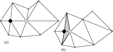
Figure 8: Two-dimensional illustration of vertex deletion from a Delaunay triangulation. In part (a), the vertex to be deleted (large hatched point) is moved in several steps followed by flips restoring the Delaunay property towards its closest neighbor (large solid point), until the inner simplices (shaded region) can be safely deleted [part (b)]. The two vertices are simply merged and the remaining opposing simplices are connected as neighbors. Finally, the Delaunay criterion is again restored by using flips.

Another problem is posed by rounding errors in (35): If the numerator becomes very small – i.e. if one has simplices with an extremely small volume or very skinny simplices, then $\lambda$ may tend to assume very small values. Rounding errors are then likely to happen as well. This problem can be weakened by using exact arithmetics [40] when computing (35) or – when working with random data – by distributing the data over a larger region of space (larger simplices). In our experiences with triangulations of reasonable data such situations actually never occurred.

We have run several tests on the deletion algorithm by first triangulating a number of points and then deleting all the points one by one. Before deleting a point we collected all simplices not containing the point (roughly speaking: the triangulation with a star-shaped hole) and checked for their existence in the resulting triangulation after point deletion. In accordance with the theorem proved in [19] they were all recovered in the final triangulation – which has also been compared with one constructed by complete re-triangulation.

3 Performance

To test our implementation, we performed calculations on a $1.533$ GHz AMD Athlon processor with 1 GByte of RAM. The code has been compiled using the GNU g$++$ 3.3 compiler with compiler optimization set. The times were then obtained using the clock() command. The seed values of the random number generator have been determined using the system time. In all test runs, the data consisted of 64-bit double variables.

3.1 Incremental Insertion Algorithm

The complexities of the walk algorithm and of the Green-Sibson algorithm have been extensively studied [20, 30]. Here we have studied the computation time in dependence of the number of points to be triangulated. Test runs were performed for different configurations of points ranging from $10^{3}$ to $10^{6}$. To avoid the handling of vertex rejection we sticked to the case of equally-weighted vertices (standard Voronoi tessellation).

In a first series of runs, we considered a slightly perturbed cubic lattice with the average lattice constant $a=1.0$ (diamonds in figure 9). As a starting simplex for the simplex walk we always took a simplex in the center of the cubus. The expected algorithmic complexity of $\alpha_{c}N^{4/3}+\beta_{c}N$ is in complete agreement with the simulation. In a second test run, we took the same lattice configuration but gave an imperfect guess for the walk algorithm (squares in fig. 9). This guess was the last simplex created and therefore good within the cubus and bad at the surface of the cubus. For large numbers of points – where the ratio between vertices at the boundary of the cubus and the total number of vertices in the cubus becomes small – we find a linear behavior, as is expected if the cost for simplex location becomes constant. To test for robustness of our code we also fed an unperturbed cubic lattice (data not shown), in this case one finds the worst-case quadratic scaling of $T_{\rm run}\approx 8.210^{-8}N^{2}$. However, in our calculations such extreme triangulations will never occur. For comparison with a uniform random distribution we triangulated different numbers of points within the cubus $[-10.0,+10.0]\times[-10.0,+10.0]\times[-10.0,+10.0]$. A much better behavior of the algorithmic complexity is found (spheres in fig. 9). Since for random data nothing is known about the final neighborships, no good guess can be given without some sort of preprocessing. However, by choosing some simplex associated with the closest vertex (out of the last 100 inserted) in analogy to [33, 34] one still finds a considerable gain in efficiency and a nearly linear scaling in the observed range (triangles in fig. 9). Furthermore, figure 9 shows that the running times for random data with our simple data structure are comparable with the more sophisticated three-dimensional DCFL data structure [7], and other code [21], where the used algorithms code scale similarly on random data.

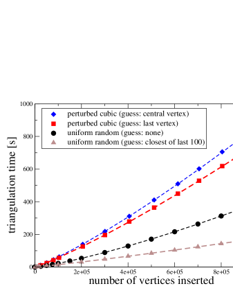
Figure 9: Times necessary for the tetrahedralization of different point numbers for different distributions. Cubic lattices are known to produce many flat simplices (called slivers). In the case of the points distributed on (perturbed) lattices, the cost of the simplex location can be reduced to constant by giving a good first guess. In the case of randomly distributed points the walk in the triangulation can be considerably shortened by choosing a better guess for a starting simplex. Dashed lines are fits with the expected overall algorithmic complexities $\alpha_{i}N^{4/3}+\beta_{i}N$.

It is evident that the incremental insertion of data points depends on the choice of the initial simplex. Figure 10 shows the increase in the average number of steps necessary for the location of the simplex containing a point using the visibility walk. The expected average $n^{1/3}$ relation is found.

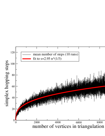
Figure 10: The number of necessary steps starting from an arbitrary simplex in the triangulation towards another arbitrary simplex scales like $n^{1/3}$. Shown is the mean out of ten runs.

3.2 Incremental Deletion Algorithm

In simulation of growth models it will often be necessary to delete vertices from a Delaunay triangulation. It turns out, that vertex deletion is more efficient than vertex insertion, since there is no cost associated with simplex location, as the vertices provide ${\mathcal{O}}\left(1\right)$ access to the incident simplices. Furthermore, one would expect the average algorithmic complexity of vertex deletion to be constant (i.e. not to depend on the total number of points). In this experiment we have first created a Delaunay triangulation and deleted it afterwards by removing point by point. Again, the mean out of ten test runs has been calculated. Figure 11 gives an impression of the expected linear relationship.

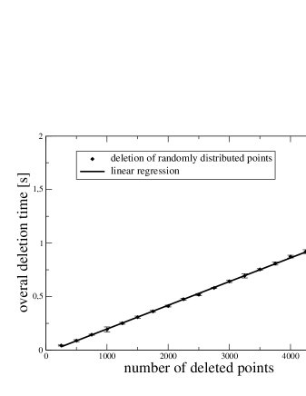
Figure 11: Calculation times necessary for the deletion of different numbers of points.

3.3 Restoring the Delaunay property

A simulation hosting kinetic vertices will be especially sensitive on the cost of checking all simplices for Delaunay invalidity and restoring the Delaunay property. We have triangulated $N\in[10^{4},10^{6}]$ random points in a vectorizable random lattice [36] (equivalent to a strongly perturbed cubic lattice) with the additional condition of a minimum distance of 0.1 between all the points. This seemed more realistic to us, since in proximity structures there will always be some minimum distance defined by the object sizes. Afterwards all points are moved by a random small step towards a hypothetical new position $\vec{X}\to\vec{X}+[RND(-m,m),RND(-m,m),RND(-m,m)]$ with $m$ chosen constant. These hypothetical new positions are put on a list, which is being iterated: Possible steps that do not invalidate the triangulation are performed instantly, the others are divided in smaller sub-steps where the criterion for the maximum step size is the same as that in section 2.5. Then the Delaunay criterion is restored (with $2\to 3$ or $3\to 2$ flips). The algorithm terminates when all new positions have been reached.

In practice, this procedure would correspond to one timestep of the application and in the ideal case (where the step sizes are small enough) just one iteration should suffice. However, the additional cost of performing a step size check before actually moving the vertices produces only a factor of roughly 2 in the restoration time and should therefore be preferred to increase the robustness of the algorithm considerably.

As expected, the complexity behaves linear in the number of points, see e.g. figure 12.

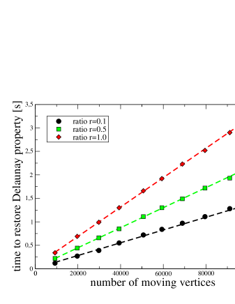
Figure 12: Shown are the calculation times necessary for the restoration of the Delaunay criterion after vertex movement for different ratios $r=m/d_{\rm min}$ (step size over the minimum distance) versus the number of points. The expected linear relation is found with slopes increasing with the step size. In the ideal case, this update method is about 20 times as fast as computing a new triangulation.

By looking at figure 12 one finds that restoring the Delaunay criterion in a slightly perturbed Delaunay triangulation being about 20 times as fast as recomputing the whole triangulation as long as the vertex displacements are small compared to the average vertex distance. Locally updating a triangulation is also faster than using a combination of delete and insert operations [35, 36], since much less simplices have to be flipped.

3.4 Mixed algorithms

To check whether a simulation can cope with a varying number of kinetic vertices, we combined the algorithms on vertex insertion, vertex deletion and vertex movement. For different numbers of uniformly distributed vertices 100 time steps have been performed. In each time step, with probability $p=0.5$ an arbitrary vertex was deleted from the triangulation and with probability $p=0.5$ a random vertex was inserted. Afterwards all the vertices were moved by a small deviation followed by the restoration of the Delaunay criterion. Therefore, if in average a constant number of vertices are deleted or inserted per timestep, we can expect an overall linear behavior as in table 1.

Table 1: Code performance for different numbers of vertices. In every run, 100 timesteps have been performed. In each timestep, with probability $p=0.5$ either an old vertex was deleted or a new vertex was inserted into the triangulation (second and third columns). Then all the vertices were moved by a small amount and the flips necessary to restore the Delaunay criterion have been counted – the fourth column does not include the flips necessary for the deletion process. In the last column, the calculation time per timestep is given.

points	deletions (total)	insertions (total)	flips (total)	one timestep [s]
20000	59	41	426	0.26
40000	51	49	1098	0.54
60000	52	48	2067	0.84
80000	46	54	2749	1.15
100000	42	58	3521	1.47
120000	47	53	5154	1.81
140000	62	38	6297	2.14
160000	56	44	7207	2.49
180000	50	50	7918	2.84
200000	49	51	9766	3.21

4 Summary

In this article we have shown that it is possible to construct fully dynamic and kinetic three-dimensional Delaunay triangulations by using a very simple data structure. This data structure is obtained by adding neighborship entries to every simplex and by storing the tetrahedra within a list. The performance of our data structure is comparable to that of more sophisticated kinetic data structures [7], which may pose an advantage for parallelization.

We have proposed a new incremental method of vertex deletion which uses a maximum step size criterion. This criterion also solves the problem of maintaining a valid three-dimensional Delaunay triangulation during vertex movement.

Note that the code allows to be generalized towards power-weighted Delaunay triangulations in a mostly straightforward way by replacing the normal circumsphere criterion by its weighted counterpart. In addition, the code provides functionality to compute volumes and contact surfaces of the associated Voronoi cells which are of importance in some simulations of interacting particle systems. The resulting tessellation of space in Voronoi/Laguerre cells can be used to model growth/shrinking processes or for the numerical solution of differential equations on irregular grids. This implementation of a fully dynamic and kinetic Delaunay triangulation thus makes our code suitable for the simulation of dynamically interacting complex systems with variable particle numbers as e.g. cell tissues.

5 Acknowledgments

G. S. is indebted to T. Beyer for discussing many aspects of the algorithms and for testing the code and to U. Brehm for discussing many theoretical problems. G. S. has been financially supported by the SMWK.

References

- [1] J. von Neumann, Theory of Self-Reproducing Automata, 1st Edition, University of Illinois Press, 1966.
- [2] R. Baer, H. Martinez, Automata and biology, Ann. Rev. Biophys. Bioeng. 3 (1974) 255–291.
- [3] M. Meyer-Hermann, A mathematical model for the germinal center morphology and affinity maturation, Journal of Theoretical Biology 216 (2002) 273–300.
- [4] F. Meineke, C. Potten, M. Loeffler, Cell migration and organization in the intestinal crypt using a lattice-free model, Cell Proliferation 34 (2001) 253–266.
- [5] M. Weliky, G. Oster, The mechanical basis of cell rearrangement, Development 109 (1990) 373–386.
- [6] M. Weliky, G. Oster, S. Minsuk, R. Keller, Notochord morphogenesis in xenopus laevis: simulation of cell behavior underlying tissue convergence and extension, Development 113 (1991) 1231–1244.
- [7] J.-A. Ferrez, Dynamic triangulations for efficient 3d simulations of granular materials, Ph.D. thesis, EPFL, thesis 2432 (2001).
- [8] A. Okabe, B. Boots, K. Sugihara, S. N. Chiu, Spatial tessellations: Concepts and applications of Voronoi diagrams, 2nd Edition, Probability and Statistics, Wiley, NYC, 2000, 671 pages.
- [9] M. D. Berg, M. van Kreveld, M. Overmars, O. Schwarzkopf, Computational Geometry, 1st Edition, Springer, Berlin, 1997.
- [10] S. Fortune, Voronoi diagrams and delaunay triangulations, Computing in Euclidean Geometry 1.
- [11] C. Lürig, T. Ertl, Adaptive iso-surface generation, 3D Image Analysis and Synthesis ’96 (1996) 183–190.
- [12] G. L. Miller, D. Talmor, S.-H. Teng, N. Walkington, A delaunay based numerical method for three dimensions: generation, formulation, and partition, Proceedings of the 27th Annual ACM Symposium on Theory of Computing (1995) 683–692.
- [13] D. C. Bottino, Computer simulations of mechanochemical coupling in a deforming domain: applications to cell motion, IMA Volumes in Mathematics and its Applications, Frontiers in Applied Mathematics Series 121 (2000) 295–314.
- [14] E. Schönhardt, Über die Zerlegung von Dreieckspolyedern in Tetraeder, Mathematische Annalen 98 (1928) 309–312.
- [15] J. Goodman, J. O’Rourke, Handbook of Discrete and Computational Geometry, 1st Edition, CRC Press, New York, 1997.
- [16] G. Brouns, A. D. Wulf, D. Constales, Multibeam data processing: Adding and deleting vertices in a delaunay triangulation, The Hydrographic Journal 101.
- [17] O. Devillers, On deletion in delaunay triangulation, Internat. J. Comput. Geom. Appl. 12 (2002) 193–205.
- [18] J. R. Shewchuk, Constrained delaunay tetrahedralizations and provably good boundary recovery, in: Eleventh International Meshing Roundtable, Sandia National Laboratories, 2002, pp. 193–204.
- [19] J. R. Shewchuk, A condition guaranteeing the existence of higher-dimensional constrained delaunay triangulations, in: Proc. of the 14th Annual Symposium on Computational Geometry, 1998, pp. 76–85.
- [20] H. Edelsbrunner, N. Shah, Incremental topological flipping works for regular triangulations, Algorithmica 15 (1996) 223–241.
- [21] E. Mücke, A robust implementation for three-dimensional delaunay triangulations, International Journal of Computational Geometry and Applications 2 (8) (1998) 255–276.
- [22] X. Xinjian, R. Franco, T. Hubert, T. Liebling, A. Mocellin, The laguerre model for grain growth in three dimensions, Philosophical Magazine B 75 (4) (1997) 567–585.
- [23] J. Sauer, Allgemeine Kollisionserkennung und Formrekonstruktion basierend auf Zellkomplexen, Ph.D. thesis, Universität des Saarlandes, Fachbereich 14 Informatik (1995).
- [24] F. Aurenhammer, H. Imai, Geometric relations among voronoi diagrams, Geom. Dedicata 27 (1988) 65–75.
-
[25]
O. Devillers, Improved incremental randomized Delaunay triangulation, in:
Proc. 14th Annu. ACM Sympos. Comput. Geom., 1998, pp. 106–115.
URL http://www-sop.inria.fr/prisme/publis/d-iirdt-98.ps.gz - [26] C. Kittel, Introduction to Solid State Physics, 7th Edition, John Wiley and Sons, 1996.
- [27] F. Aurenhammer, Voronoi diagrams – a survey of fundamental geometric data structure, ACM Computing Surveys 23 (3) (1991) 345–405.
- [28] J.-D. Boissonnat, M. Teillaud, On the randomized construction of the delaunay tree, Theoretical Computer Science 112 (2) (1993) 339–354.
- [29] T. J. Choi, Generating optimal computational grids: Overview and review, http://www.me.cmu.edu/faculty1/shimada/cg97/taek/ (1997).
- [30] O. Devillers, S. Pion, M. Teillaud, Walking in a triangulation, in: Proc. 17th Annu. Sympos. Comput. Geom., 2001, pp. 106–114.
- [31] M. A. Facello, Constructing delaunay and regular triangulations in three dimensions, Ph.D. thesis, University of Illinois at Urbana-Champaign (1993).
- [32] A. Bowyer, Computing dirichlet tessellations, The Computer Journal 24 (2) (1981) 162–166.
- [33] E. P. Mücke, I. Saias, B. Zhu, Fast randomized point location without preprocessing in two- and three-dimensional delaunay triangulations, in: Proc. 12th Annu. ACM Sympos. Comput. Geom., 1996, pp. 274–283.
- [34] L. Devroye, E. P. Mücke, B. Zhu, A note on point location in delaunay triangulations of random points, Algorithmica 22 (1998) 477–482.
- [35] G. D. Fabritiis, P. V. Coveney, Dynamical geometry for multiscale dissipative particle dynamics, arXiv:cond-mat/0301378 .
- [36] K. B. Lauritsen, H. Puhl, H.-J. Tillemans, Performance of random lattice algorithms, International Journal of Modern Physics C 5 (6) (1994) 909–922.
- [37] M. A. Mostafavi, C. Gold, M. Dakowicz, Delete and insert operations in voronoi/delaunay methods and applications, Computers & Geosciences 29 (2003) 523–530.
- [38] J.-D. Boissonnat, M. Yvinec, Algorithmic Geometry, 1st Edition, Cambridge University Press, Cambridge, 1998.
- [39] M. Vigo, N. Pla, Regular triangulations of dynamic sets of points (2000).
- [40] O. Devillers, S. Pion, Efficient exact geometric predicates for delaunay triangulations, in: Proc. 5th Workshop Algorithm Eng. Exper., 2003, pp. 37–44.