Localized helium excitations in ⁴He_N-benzene clusters

Abstract

We compute ground and excited state properties of small helium clusters ⁴He_N containing a single benzene impurity molecule. Ground-state structures and energies are obtained for $N=1,2,3,14$ from importance-sampled, rigid-body diffusion Monte Carlo (DMC). Excited state energies due to helium vibrational motion near the molecule surface are evaluated using the projection operator, imaginary time spectral evolution (POITSE) method. We find excitation energies of up to $\sim 23$ K above the ground state. These states all possess vibrational character of helium atoms in a highly anisotropic potential due to the aromatic molecule, and can be categorized in terms of localized and collective vibrational modes. These results appear to provide precursors for a transition from localized to collective helium excitations at molecular nanosubstrates of increasing size. We discuss the implications of these results for analysis of anomalous spectral features in recent spectroscopic studies of large aromatic molecules in helium clusters.

I Introduction

Helium droplets provide a unique, ultra-cold nanolaboratory for investigation of a variety of physical and chemical phenomena.Toennies et al. (2001) This has been increasingly used in recent years to analyze the behavior of a wide variety of atomic and molecular species in a quantum liquid environment, using spectroscopic techniques to probe both the molecular and helium dynamics.spe Electronic spectroscopy in particular allows one to probe microscopic details of the helium dynamics. In the large droplet regime ($N\geq 10^{3}$), the laser-induced fluorescence (LIF) spectra of molecules in cold helium droplets are usually characterized by a sharp zero-phonon line (ZPL) due to the transition for the electronic origin, accompanied by a broad, phonon wing sideband. The zero-phonon line can contain fine structure due to internal molecular transitions, while the phonon wing structure reflects the coupling to collective excitations of the surrounding helium. Thus, electronic excitation spectrum of glyoxal, a small 6-atom molecule (C₂H₂O₂), in ⁴He droplets at $T=0.38$ K, exhibits a distinct phonon wing feature that is separated by a gap from the zero-phonon transition.Hartmann et al. (1996) In contrast, in ³He droplets the corresponding spectrum shows a phonon wing feature but no gap.Grebenev et al. (2000) The phonon wing structure for glyoxal in has been successfully interpreted in terms of excitation of the collective phonon-roton modes in large ⁴He droplets,Hartmann et al. (1996) while the lack of a gap between zero phonon and phonon wing features in ³He droplets has been interpreted as consistent with the presence of particle-hole excitations in normal ³He.Grebenev et al. (2000) Recent spectroscopic experiments involving larger organic molecules in ⁴He_N clusters have revealed interesting additional features beyond these basic elements.Stienkemeier and Vilesov (2001) For a number of the larger organic molecules studied so far, both the ZPL and phonon wing portions of the LIF spectra exhibit sharp peaks superimposed on the underlying features. These additional peaks are not compatible with this basic picture of molecular electronic excitation coupling to either internal molecular transitions or bulk compressional modes of helium.Hartmann et al. (1998, 2001); Lindinger et al. (2001); Hartmann et al. (2002)

In addition to these experiments in large helium droplets, a new class of size-selective experiments involving small numbers ($N\leq 20$) of ⁴He atoms attached to large planar aromatic molecules has also recently emerged.Even et al. (2000, 2001) These small cluster studies allow one to directly observe the size evolution of excited states involving helium motion, at sizes less than a full solvation shell around the molecule. For these small clusters, which are better described as weakly bound complexes with helium than as quantum solvated molecules, a very different situation pertains. Starting with $N=1$, the experimental spectra show discrete lines that generally increase in complexity with increasing $N$, with the number of observed lines reaching a maximum at $N\sim 4-5$. After this, many of the discrete features observed for smaller $N$ disappear, until only a few lines persist at $N\sim 10$.

The larger organic molecules that have been studied experimentally vary in complexity from planar aromatics such as tetracene (a fused conjugated system of four six-membered carbon rings connected by common bonds)Hartmann et al. (1998, 2001) to more complex heterostructures such as phthalocyanineHartmann et al. (2002) and indole derivatives.Lindinger et al. (2001) The presence of aromatic character due to $\pi$-electron conjugation provides a common feature in these systems. Because of their geometry and $\pi$-electron character, planar aromatics such as tetracene are particularly interesting for study in helium droplets because they can be considered as nanoscale precursors to a bulk graphite surface and their local quantum solvation structure concomitantly as a nanoscale precursor of the adsorption behavior of thin helium films on graphite. A considerable body of literature has been accumulated for helium films on graphite,Bretz et al. (1973); Shirron and Mochel (1991); Greywall and Busch (1991); Zimmerli et al. (1992); Adams and Pant (1992); Clements et al. (1993); Wagner and Ceperley (1994); Dalfovo et al. (1995); Csáthy et al. (1998); Nyéki et al. (1998); Pierce and Manousakis (1999) so that analysis of the solvation structure and helium excitations as a function of increasing size of polyaromatic molecule offers the possibility of developing a microscopic understanding of the evolution from quantum solvation of an isolated molecule, to adsorption and film formation at a bulk surface in superfluid helium.

The unusual features recorded in experimental spectra for these organic molecules consist of unidentified peaks in the phonon wings of vibronic bandsHartmann et al. (2002) and anomalous splittings of the zero-phonon lines.Hartmann et al. (1998, 2001); Lindinger et al. (2001) It has been speculated that both of these types of features may be due to some type of excitation of helium atoms that are localized at the molecular surface,Hartmann et al. (2001); Lindinger et al. (2001); Hartmann et al. (2002) but the true origin of both of these types of features is unclear. Supporting evidence for excitations of localized helium atoms derives from the similarity of the energies for phonon wing peaks with low-frequency modes of thin films on graphite ($4-11$ K) observed via neutron scattering Lauter et al. (1992); Clements et al. (1996) as well as from theoretical predictions of spatially localized helium atoms at an aromatic ring in the benzene molecule.Kwon and Whaley (2001) Path integral calculations reveal this to be a true localization of helium atoms that are effectively completely removed from participation in the superfluid, thereby constituting a single ”dead” atom in the surrounding solvation layer. The characteristics of excitations of such localized helium atoms around aromatic substrates are expected to be very different from the collective helium modes found in large droplets,Krishna and Whaley (1990); Chin and Krotscheck (1992, 1995) but to show increasing similarity with surface localized modes in helium filmsLauter et al. (1992); Clements et al. (1996) as the size of the molecular nanosubstrate increases.

Theoretical analysis of the phenomenology of these helium excitations near a molecular nanosubstrate is rendered difficult due both to the lack of accurate interaction potentials for these larger molecules with helium, and to the need for accurate calculation of excited states in a very inhomogeneous quantum liquid environment. Only a few direct calculations to elucidate the nature of these helium excitations in the presence of a large molecular impurity have been reported so far, and these have been restricted to very small numbers of helium atoms ($N=1,2$).Bach et al. (1997); Anderson et al. (2000); Heidenreich et al. (2001) Calculations involving doped clusters require accurate helium-impurity potential energy surfaces, of which there is a definite lack for the larger organic molecules. Thus, most calculations with large molecules resort to the use of simple atom-atom pair potential models. Given a potential surface, excited state calculations employing basis set methods are still limited to small $N$, where $N$ is typically no greater than two.Bach et al. (1997); Anderson et al. (2000); Heidenreich et al. (2001) For larger numbers of helium atoms that are however not yet in the regime of bulk films, a practical approach is provided by calculations for excited states that are based on quantum Monte Carlo methods.

In this work, we present a series of such quantum Monte Carlo studies of the ground and excited states of small helium clusters $(N=1,2,3,14)$ containing a benzene impurity. Benzene is a simple planar aromatic molecule, and it can be viewed as a primitive $sp^{3}$-hybridized unit of a bulk graphite surface. Thus, it is the logical starting point for the kind of systematic study of helium adsorption on molecular nanosubstrates mentioned above. We note that this notion has been pursued extensively for the heavier noble gases,Leutwyler and Jortner (1987) but it is only recently that experimental data for helium has become available. We employ here both the well-known ground-state diffusion Monte Carlo method and the projection operator imaginary time spectral evolution (POITSE) method for excited states.Blume et al. (1997) The latter approach allows exact excitation energies to be obtained, provided a high-quality trial function approximating the ground state is available. We calculate a range of helium excitation energies at $T=0$ K and analyze these in terms of their spatial nature and extent. The previous path integral calculations for the ⁴He₃₉-benzene system at a temperature of $T=0.625$ K have shown that the effect of the strength and strong $\pi$-anisotropy of the He-benzene interaction serves to localize a single helium atom on each side of the benzene surface.Kwon and Whaley (2001) That is, in the Feynman path integral representation, a single helium atom attached to the benzene surface is completely removed from permutation exchanges with the surrounding helium environment. In this work, we find a set of collective helium vibrations which have energies of up to $\sim 23$ K above the ground state, and can be characterized in terms of their transformation properties under the symmetry group of the He-benzene interaction potential. We show that even for sizes as small as $N=14$ helium atoms, one can distinguish a subset of higher-energy excitations localized near the global minimum of the helium-benzene interaction potential, from a subset of lower-energy collective excitations which are delocalized around the periphery of the molecule surface. The former appear to be associated with the localized helium density identified from path integral calculations in Ref. Kwon and Whaley, 2001.

Sec. II begins with a discussion of the model Hamiltonian and potential surface. Technical details of the quantum Monte Carlo methodology are presented in Sec. III. Our results for ground and excited states of ⁴He_N-benzene ($N=1,2,3,14$) are presented in Sec. V, where we analyze the nature of these molecule-induced localized states around the benzene impurity and, and in Sec. VI we discuss the implications for helium excitations on larger aromatic molecules.

II The model Hamiltonian

We treat the ⁴He_N-benzene cluster as a collection of $N$ indistinguishable helium atoms, and a rigid benzene molecule which is free to translate and rotate in space. Thus the benzene intramolecular degrees of freedom are held fixed, which implicitly assumes a separation between the helium motion and the benzene vibrational modes. The positions of the $N$ helium atoms in a space-fixed (SF) frame of reference are denoted as $\{\mathbf{R}_{1},\mathbf{R}_{2},\ldots,\mathbf{R}_{N}\}$, and the SF position of the benzene center-of-mass is denoted as $\mathbf{R}_{I}$. The Hamiltonian $\hat{H}$ is $(3N+6)$–dimensional: there are $3N$ helium translational degrees of freedom, plus an additional six dimensions due to translation and rigid-body rotation of the benzene molecule. It takes the form

$$\hat{H}=\hat{T}^{(\mathrm{imp})}+\hat{T}^{(\mathrm{He})}+\hat{V},$$ (1)

where $\hat{T}^{(\mathrm{imp})}$, $\hat{T}^{(\mathrm{He})}$, and $\hat{V}$ are the impurity rigid-body kinetic energy, helium kinetic energy, and total potential energy, respectively. The impurity kinetic energy is most easily expressed by introducing a moving body-fixed (BF) frame $(\hat{x},\hat{y},\hat{z})$, whose origin relative to the SF frame is fixed at the benzene center-of-mass ${\bf R}_{I}$. The Euler angles $(\varphi,\vartheta,\chi)$ specify the orientation of the BF axes, which are set parallel to the benzene principal axes. The benzene kinetic energy is thus

$$\hat{T}^{(\mathrm{imp})}=-D_{I}\nabla_{I}^{2}-d_{a}\left(\frac{\partial^{2}}{\partial\phi_{x}^{2}}+\frac{\partial^{2}}{\partial\phi_{y}^{2}}\right)-d_{c}\frac{\partial^{2}}{\partial\phi_{z}^{2}},$$ (2)

with the prefactors

$$D_{I}=\frac{\hbar^{2}}{2m_{I}},\ d_{a}=\frac{\hbar^{2}}{2I_{a}},\ d_{c}=\frac{\hbar^{2}}{2I_{c}}.$$ (3)

The first term of $\hat{T}^{(\mathrm{imp})}$ is the center-of-mass translational kinetic energy for a benzene molecule, where we use a mass $m_{I}=78.114$ amu. The remaining terms give the benzene rigid-body rotational kinetic energy, where the prefactors $d_{a}=0.188$ cm^-1 and $d_{c}=0.0938$ cm^-1 are the (oblate) symmetric top rotational constants. The Laplacian $\nabla_{I}^{2}$ is taken with respect to the translations of the benzene center-of-mass. The angular second derivatives are taken with respect to rotations of the benzene about the BF axes $(\hat{x},\hat{y},\hat{z})$. Similarly, the next term of the Hamiltonian is the helium kinetic energy,

$$\hat{T}^{(\mathrm{He})}=-D_{4}\sum_{j=1}^{N}\nabla_{j}^{2},\ D_{4}=\frac{\hbar^{2}}{2m_{4}},$$ (4)

where $m_{4}$ is the ⁴He mass, and $\nabla_{j}^{2}$ denotes the Laplacian taken with respect to the displacement of helium atom $j$.

The final term of Eq. (1) is the model potential energy. We use an additive, two-body potential,

$$\hat{V}=\sum_{j=1}^{N}V_{\mathrm{He-I}}(\mathbf{r}_{j})+\sum_{i<j}^{N}V_{\mathrm{He-He}}(r_{ij}).$$ (5)

The helium-helium interaction $V_{\mathrm{He-He}}$ is given by the semi-empirical HFD-B potential of Aziz et al.,Aziz et al. (1987) and depends only on the distance $r_{ij}$ between helium atoms $i,j$. The helium-benzene interaction $V_{\mathrm{He-I}}$ is most conveniently expressed in terms of helium BF frame coordinates $\{\mathbf{r}_{1},{\bf r}_{2},\ldots,\mathbf{r}_{N}\}$. It is an analytical fit to ab initio MP2 data of Hobza et al.,Hobza et al. (1992) and consists of a sum of atom-atom terms:

$$V_{\mathrm{He-I}}(\mathbf{r}_{j})=\sum_{\alpha=1}^{6}V_{\mathrm{C}}(\mathbf{r}_{\alpha j})+\sum_{\beta=1}^{6}V_{\mathrm{H}}(r_{\beta j}).$$ (6)

The indices $\alpha$ and $\beta$ run over the carbon and hydrogen atoms of the benzene molecule, respectively. The helium-hydrogen interaction $V_{\mathrm{H}}$ is a standard Lennard-Jones 6-12 form which depends on the distance $r_{\beta j}$ between hydrogen atom $\beta$ and helium atom $j$,

$$V_{\mathrm{H}}(r_{\beta j})=4\epsilon_{\mathrm{H}}\left[\left(\frac{\sigma_{\mathrm{H}}}{r_{\beta j}}\right)^{12}-\left(\frac{\sigma_{\mathrm{H}}}{r_{\beta j}}\right)^{6}\right].$$ (7)

The helium-carbon interaction $V_{\mathrm{C}}$ has a modified angle-dependent Lennard-Jones 8-14 form,

$$V_{\mathrm{C}}(\mathbf{r}_{\alpha j})=4\epsilon^{\prime}_{\mathrm{C}}\left[\left(\frac{\sigma^{\prime}_{\mathrm{C}}}{r_{\alpha j}}\right)^{14}-\left(\frac{\sigma^{\prime}_{\mathrm{C}}}{r_{\alpha j}}\right)^{8}\right],$$ (8)

where $\epsilon^{\prime}_{\mathrm{C}}=\epsilon_{\mathrm{C}}\cos^{2}\theta$, $\sigma^{\prime}_{\mathrm{C}}=\sigma_{\mathrm{C}}\cos\theta$, and $\theta$ is the spherical polar angle with respect to a coordinate frame centered on the carbon atom $\alpha$ and parallel to the BF frame. The potential fit parameters are listed in Table 1.

Table 1: Helium-benzene potential parameters. The carbon-carbon and carbon-hydrogen bond lengths are held fixed at $r_{\mathrm{CC}}$ and $r_{\mathrm{CH}}$, respectively, and all bond angles are 120^∘.

$\epsilon_{\mathrm{C}}$	$15.25~{}K$
$\sigma_{\mathrm{C}}$	$3.59~{}\AA$
$\epsilon_{\mathrm{H}}$	$19.14~{}K$
$\sigma_{\mathrm{H}}$	$2.69~{}\AA$
$r_{\mathrm{CC}}$	$1.406~{}\AA$
$r_{\mathrm{CH}}$	$1.08~{}\AA$

This helium-benzene potential possesses two equivalent global minima of $-94.97$ K at $z=\pm 3.27$ Å along the benzene $C_{6}$-axis. There are also 12 equivalent secondary minima of $-62.54$ K located between neighboring hydrogen atoms, six above and six below the benzene plane. The global minima are connected to the secondary minima by saddle points of $-50.77$ K, situated approximately above and below the C–H bonds. A cut of the potential at $z=3.27$ Å is shown in the top panel of Fig. 1,

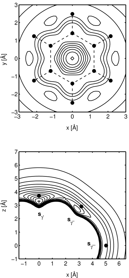
Figure 1: Top: cut of the ⁴He-benzene potential through the global minima at $z=3.27$ Å. The carbon and hydrogen $(x,y)$ positions are marked with solid circles and connected by dashed lines. Bottom: cut of the same potential at $y=0$. Three representative sites $\mathbf{s}_{\gamma^{\prime}},\mathbf{s}_{\gamma^{\prime\prime}},\mathbf{s}_{\gamma^{\prime\prime\prime}}$ are marked, which correspond to centers of the helium-benzene localization factors centered near the global, secondary, and tertiary potential minima, respectively (Secs. IV and V.1).

where the $(x,y)$ positions of the carbon and hydrogen atoms on the $z=0$ plane are also marked. The lower panel of Fig. 1 shows a cut of the potential along the $y=0$ plane, which reveals one of the secondary minima at $x=2.84$ Å, $z=2.70$ Å, and one of the saddle points at $x=1.97$ Å, $z=3.54$ Å.

For $N=1$, the model Hamiltonian of Eq. (1) belongs to the molecular symmetry group $D_{6h}(M)$, which is the subgroup consisting of only the feasible elements of the complete nuclear permutation and inversion group (CNPI).Bunker and Jensen (1998) This group is isomorphic to the $D_{6h}$ point group, which is valid in the limit of small amplitude helium motions. For $N>1$, the symmetry group is identically $D_{6h}(M)$ due to Bose symmetry, since the only allowed rovibrational states are those obtained from the tensor product of irreducible representations of $D_{6h}(M)$, with irreducible representations of the symmetric group $S_{N}$ which remain unchanged under permutation of identical ⁴He nuclei, i.e. the totally symmetric representation of $S_{N}$.

III Computational methodology

In this section we present a summary of the numerical methods employed in our study of the ⁴He_N-benzene system. Variational estimates of ground-state energies are obtained from variational Monte Carlo (VMC), and exact ground-state properties are computed from diffusion Monte Carlo (DMC) with importance sampling.Hammond et al. (1994); Viel et al. (2002) The projection operator, imaginary time spectral evolution (POITSE) approach is used to obtain excited-state energies.Blume et al. (1997) Both the DMC and POITSE methods can provide results that are exact, to within a systematic time step error.

III.1 Ground states: variational Monte Carlo (VMC)

The starting point for our study of the ⁴He_N-benzene system begins with the Rayleigh-Ritz variational theorem,

$$E_{T}=\frac{\langle\Psi_{T}|\hat{H}|\Psi_{T}\rangle}{\langle\Psi_{T}|\Psi_{T}\rangle}\geq E_{0},$$ (9)

where the trial energy $E_{T}$ with respect to some parameterized trial function $\Psi_{T}$ represents an upper bound to the exact ground-state energy $E_{0}$. In the coordinate representation, this becomes

$$E_{T}=\frac{\int d\mathcal{R}\,\Psi_{T}^{2}(\mathcal{R})E_{L}(\mathcal{R})}{\int d\mathcal{R}\,\Psi_{T}^{2}(\mathcal{R})},$$ (10)

where $\mathcal{R}$ is a $(3N+6)$–dimensional coordinate denoting the positions and orientations of all bodies governed by the Hamiltonian $\hat{H}$. The quantity $E_{L}$ is a local energy, defined as

$$E_{L}(\mathcal{R})=\Psi_{T}^{-1}(\mathcal{R})\hat{H}\Psi_{T}(\mathcal{R}).$$ (11)

An optimized variational upper bound is obtained by varying the parameters of $\Psi_{T}$ to minimize $E_{T}$.

For a realistic $N$-particle helium system, Monte Carlo methods offer a practical means to compute the multidimensional integral of Eq. (10). In variational Monte Carlo, expectation values of observables are evaluated as averages over the normalized distribution

$$f(\mathcal{R})=\frac{\Psi_{T}^{2}(\mathcal{R})}{\int d\mathcal{R}\,\Psi_{T}^{2}(\mathcal{R})},$$ (12)

which is numerically represented as a discrete ensemble of Monte Carlo walkers $\{\mathcal{R}_{k}\}$. Typically, we use an ensemble size of $n_{w}=2000$ walkers. This distribution can be generated from a Metropolis walk, in which a move $\mathcal{R}\rightarrow\mathcal{R}^{\prime}$ is proposed with a transition probability consisting of factors having the form

$$G_{D}(\mathbf{R}_{j}\rightarrow\mathbf{R}_{j}^{\prime},\Delta\tau)=\\ \left(\frac{1}{4\pi D\Delta\tau}\right)^{3/2}\exp\left\{-\frac{[\mathbf{R}_{j}^{\prime}-\mathbf{R}_{j}-D\Delta\tau\mathbf{F}_{j}(\mathcal{R})]^{2}}{4D\Delta\tau}\right\}.$$ (13)

The vector quantity $\mathbf{F}$ is commonly referred to as the “quantum force”, and is chosen to be

$$\mathbf{F}_{j}(\mathcal{R})=2\Psi_{T}^{-1}(\mathcal{R})\nabla_{j}\Psi_{T}(\mathcal{R}).$$ (14)

$G_{D}$ can be viewed as the Green’s function associated with a diffusion/drift process in the presence of an external field $\mathbf{F}$, over a time step of $\Delta\tau$. All VMC-based computations reported here use a time step of $\Delta\tau=75-100$ Hartree^-1. For the ⁴He_N-benzene system the full $(3N+6)$–dimensional transition probability is comprised of $N$ such factors with diffusion constant $D=D_{4}$ corresponding to the $N$ helium atoms, a factor with $D=D_{I}$ corresponding to the benzene impurity, and three analogous one-dimensional factors corresponding to individual rotations of the benzene about each of its three principal axes. A proposed move $\mathcal{R}\rightarrow\mathcal{R}^{\prime}$ is subsequently accepted with probability $p=\min(1,q)$, where the acceptance ratio $q$ is

$$q=\frac{\Psi_{T}^{2}(\mathcal{R}^{\prime})}{\Psi_{T}^{2}(\mathcal{R})}\frac{G_{D}(\mathcal{R}^{\prime}\rightarrow\mathcal{R},\Delta\tau)}{G_{D}(\mathcal{R}\rightarrow\mathcal{R}^{\prime},\Delta\tau)}.$$ (15)

With the choice of transition and acceptance probabilities given by Eqs. (13)–(15), the Metropolis walk converges to the asymptotic distribution $\Psi_{T}^{2}(\mathcal{R})$. At this point, expectation values for quantities such as the variational trial energy $E_{T}$ are sampled from this distribution as

$$E_{T}=\langle E_{L}\rangle=\left\langle\frac{1}{n_{w}}\sum_{k=1}^{n_{w}}E_{L}(\mathcal{R}_{k})\right\rangle_{\mathrm{walk}},$$ (16)

where the notation $\langle\ldots\rangle_{\mathrm{walk}}$ denotes a statistical average over the course of the equilibrated Metropolis walk. This is performed by sampling the quantity given in $\langle\ldots\rangle_{\mathrm{walk}}$ every $M$ time steps apart, with $M$ chosen to be longer than the autocorrelation length in order to minimize correlation biases in the error estimates; typically $M=50$ for our VMC computations here.

III.2 Ground states: diffusion Monte Carlo (DMC)

With diffusion Monte Carlo (DMC), one can move beyond the variational level of theory to obtain exact ground-state expectation values for the energy and quantities which commute with the Hamiltonian $\hat{H}$. This method derives from the imaginary time $(\tau=it/\hbar)$ Schrödinger equation,

$$-\frac{\partial\Psi(\mathcal{R},\tau)}{\partial\tau}=(\hat{H}-E_{\mathit{r}ef})\Psi(\mathcal{R},\tau),$$ (17)

where $\Psi(\mathcal{R},\tau)$ is the many-body wave function, and $E_{\mathit{r}ef}$ is an arbitrary constant shift in the energy spectrum. Importance sampling is introduced by multiplying both sides of Eq. (17) by a trial function $\Psi_{T}(\mathcal{R})$, and rewriting in terms of $f(\mathcal{R},\tau)=\Psi_{T}({\mathcal{R}})\Psi(\mathcal{R},\tau)$ to obtain a set of equations having the form

$$-\frac{\partial f(\mathcal{R},\tau)}{\partial\tau}=-D\nabla_{j}^{2}f(\mathcal{R},\tau)+D\nabla_{j}\cdot\mathbf{F}_{j}(\mathcal{R})f(\mathcal{R},\tau)\\ +[E_{L}(\mathcal{R})-E_{\mathit{r}ef}]f(\mathcal{R},\tau).$$ (18)

The stationary solution is now the normalized “mixed” distribution

$$f(\mathcal{R})=\frac{\Psi_{T}(\mathcal{R})\phi_{0}(\mathcal{R})}{\int d\mathcal{R}\,\Psi_{T}(\mathcal{R})\phi_{0}(\mathcal{R})},$$ (19)

where $\phi_{0}$ is the exact many-body ground-state wave function. In DMC, the approximate short-time Green’s function $G$ which generates this distribution is

$$G(\mathcal{R}\rightarrow\mathcal{R}^{\prime},\Delta\tau)\approx G_{D}(\mathcal{R}\rightarrow\mathcal{R}^{\prime},\Delta\tau)G_{B}(\mathcal{R}\rightarrow\mathcal{R}^{\prime},\Delta\tau).$$ (20)

Here, $G_{D}$ is the diffusion/drift Green’s function of Eq. (13), and $G_{B}$ has the form

$$G_{B}(\mathcal{R}\rightarrow\mathcal{R}^{\prime},\Delta\tau)=\\ \exp\left\{-\left[\frac{E_{L}(\mathcal{R})+E_{L}(\mathcal{R}^{\prime})}{2}-E_{\mathit{r}ef}\right]\Delta\tau\right\}.$$ (21)

All DMC-based computations here use a time step of $\Delta\tau=25$ Hartree^-1. A proposed move $\mathcal{R}\rightarrow\mathcal{R}^{\prime}$ is accepted or rejected according to Eq. (15), to ensure that the exact ground state is sampled in the limit of perfect importance sampling, i.e. when $\Psi_{T}(\mathcal{R})=\phi_{0}(\mathcal{R})$. For a non-exact trial function however, the approximate Green’s function of Eq. (20) results in a systematic time step error.

Operationally, the importance-sampled DMC procedure is similar to that described previously for VMC, except now associated with each walker $\mathcal{R}_{k}$ is a cumulative weight $w_{k}$ due to the action of $G_{B}$:

$$w_{k}=\prod_{n=1}^{n_{\tau}}G_{B}(\mathcal{R}_{k}\rightarrow\mathcal{R}_{k}^{\prime},n\Delta\tau).$$ (22)

The efficiency of the DMC method can be significantly improved by replicating walkers with large $w_{k}$, and destroying walkers with small $w_{k}$. At every $10-50$ time steps, the ensemble is checked for walkers whose weight exceeds the empirically set bounds $w_{\mathit{m}in}$ and $w_{\mathit{m}ax}$. A walker $\mathcal{R}_{k}$ with weight $w_{k}>w_{\mathit{m}ax}$ is replicated into $n_{k}=\mathrm{int}(w_{k}+u)$ walkers, where $u$ is a uniform random number on $[0,1)$. These new walkers are then assigned the weight $w_{k}/n_{k}$. A walker ${\mathcal{R}}_{k}$ with weight $w_{k}<w_{\mathit{m}in}$ is destroyed with probability $1-w_{k}$; otherwise its weight is set to unity. This is to ensure that the branching scheme, on average, does not artificially alter the ensemble sum of weights $W_{\mathit{t}ot}=\sum w_{k}$. The parameters $w_{\mathit{m}in}$ and $w_{\mathit{m}ax}$ are chosen empirically to maintain a stable DMC walk with respect to $W_{\mathit{t}ot}$ and the ensemble size; here we use $w_{\mathit{m}in}=0.1-0.3$ and $w_{\mathit{m}ax}=2.0-2.2$. Additionally, we also vary the reference energy $E_{\mathit{r}ef}$ during the course of the walk according to

$$E_{\mathit{r}ef}(\tau+\Delta\tau)=E_{\mathit{r}ef}(\tau)+\frac{\eta}{\Delta\tau}\ln\left[\frac{W_{\mathit{t}ot}(\tau)}{W_{\mathit{t}ot}(\tau+\Delta\tau)}\right].$$ (23)

Here, the imaginary-time dependence of the $E_{\mathit{r}ef}$ and $W_{\mathit{t}ot}$ is explicitly written. We set $E_{\mathit{r}ef}$ initially to be the starting ensemble average for the local energy $\langle E_{L}\rangle$. The empirical update parameter $\eta$ is chosen to be as small as possible, typically $\eta/\Delta\tau=0.0004-0.004$, which gives fluctuations in $W_{\mathit{t}ot}$ of roughly 5%.

Once the ensemble converges to the mixed distribution $\Psi_{T}(\mathcal{R})\phi_{0}(\mathcal{R})$, mixed expectation values for a Hermitian observable $\hat{O}$ can be obtained as

$$\langle\hat{O}\rangle_{\mathrm{mix}} =\left\langle\frac{1}{W_{\mathit{t}ot}}\sum_{k=1}^{n_{w}}w_{k}\Psi_{T}^{-1}(\mathcal{R}_{k})\hat{O}\Psi_{T}(\mathcal{R}_{k})\right\rangle_{\mathrm{walk}}$$ (24)

$$=\frac{\int d\mathcal{R}\,\Psi_{T}(\mathcal{R})\phi_{0}(\mathcal{R})\Psi_{T}^{-1}(\mathcal{R})\hat{O}\Psi_{T}(\mathcal{R})}{\int d\mathcal{R}\,\Psi_{T}(\mathcal{R})\phi_{0}(\mathcal{R})}$$ (25)

$$=\frac{\langle\phi_{0}|\hat{O}|\Psi_{T}\rangle}{\langle\phi_{0}|\Psi_{T}\rangle}.$$ (26)

In our ground-state DMC calculations, this average is computed by sampling $\hat{O}$ every $M=150$ time steps apart, which is larger than that used for VMC because successive DMC iterations are more strongly correlated due to the smaller DMC time steps that we use here. In the case where $\phi_{0}$ is an eigenstate of $\hat{O}$, i.e. when $\hat{O}$ commutes with the Hamiltonian $\hat{H}$, this procedure yields exact expectation values. All ground-state energies reported in this work are derived from the mixed estimator for the local energy, and are thus exact. For quantities which do not commute with $\hat{H}$, such as the local helium density operator $\hat{\rho}(\mathbf{r})=\sum_{j}\delta(\mathbf{r}-\mathbf{r}_{j})$, the mixed estimator is biased by the trial function $\Psi_{T}$. But as pointed out by Liu et al.,Liu et al. (1974) the asymptotic weight $w_{k}(\tau\rightarrow\infty)$ of a walker $\mathcal{R}_{k}$ is proportional to $\phi_{0}(\mathcal{R}_{k})/\Psi_{T}(\mathcal{R}_{k})$. Thus, in principle this trial function bias can be eliminated by computing instead the reweighted average

$$\langle\hat{O}\rangle =\frac{\sum_{k=1}^{n_{w}}w_{k}(\tau)w_{k}(\tau+M^{\prime}\Delta\tau)\Psi_{T}^{-1}(\mathcal{R}_{k})\hat{O}\Psi_{T}(\mathcal{R}_{k})}{\sum_{k=1}^{n_{w}}w_{k}(\tau)w_{k}(\tau+M^{\prime}\Delta\tau)}$$ (27)

$$=\cfrac{\int d\mathcal{R}\,\Psi_{T}(\mathcal{R})\phi_{0}(\mathcal{R})\Psi_{T}^{-1}(\mathcal{R})\hat{O}\Psi_{T}(\mathcal{R})\cfrac{\phi_{0}(\mathcal{R})}{\Psi_{T}(\mathcal{R})}}{\int d\mathcal{R}\,\Psi_{T}(\mathcal{R})\phi_{0}(\mathcal{R})\cfrac{\phi_{0}(\mathcal{R})}{\Psi_{T}(\mathcal{R})}}$$ (28)

$$=\langle\phi_{0}|\hat{O}|\phi_{0}\rangle,$$ (29)

where $M^{\prime}$ is taken to be as large as possible, typically $M^{\prime}=1500$. When branching processes are incorporated in the DMC, one needs to take care to keep track of walkers that descended from a walker $\mathcal{R}_{k}$ at time $\tau$. All helium densities reported in this work ($N\leq 14$) are computed by reweighting walkers $\mathcal{R}_{k}$ by their descendant weights, i.e. using Eq. (27). However, the statistical noise seen in the densities computed in this manner is much greater than from densities obtained using the mixed estimator, and thus this approach becomes problematic for ⁴He_N-benzene at still larger sizes.

III.3 Excited states: projection operator imaginary time spectral evolution (POITSE)

The POITSE approach is a DMC-based method which can provide exact excited state energies, subject to a systematic time step bias.Blume et al. (1997) It begins with the DMC evaluation of the imaginary-time correlation function

$$\tilde{\kappa}(\tau) =\frac{\langle\Psi_{T}|\hat{A}e^{-(\hat{H}-E_{\mathit{r}ef})\tau}\hat{A}^{\dagger}|\Psi_{T}\rangle}{\langle\Psi_{T}|e^{-(\hat{H}-E_{\mathit{r}ef})\tau}|\Psi_{T}\rangle}$$ (30)

$$\propto\sum_{n}|\langle\phi_{n}|\hat{A}^{\dagger}|\Psi_{T}\rangle|^{2}e^{-(E_{n}-E_{0})\tau}+O(x^{2})$$ (31)

where

$$x=\frac{\langle\Psi_{T}|\phi_{m}\rangle}{\langle\Psi_{T}|\phi_{0}\rangle}.$$ (32)

Here, $\{\phi_{n}\}$ and $\{E_{n}\}$ represent a complete set of energy eigenstates and eigenvalues of the Hamiltonian $\hat{H}$, respectively, and $\hat{A}^{\dagger}$ is an operator chosen to connect $\Psi_{T}$ to the excited state(s) of interest $\phi_{n}$. $\Psi_{T}$ should be a good approximation to the exact ground state $\phi_{0}$. To second order in $x$, $\tilde{\kappa}(\tau)$ is a superposition of exponential decays whose decay rates correspond to the energy differences $E_{n}-E_{0}$.Blume (1998); Huang et al. (2002) The VMC procedure of Sec. III.1 is used to generate an initial ensemble of $n_{w}=2000$ walkers distributed according to $f(\mathcal{R},0)\propto\Psi_{T}^{2}(\mathcal{R})$. This distribution is then propagated in imaginary time using the DMC procedure outlined in Sec. III.2, during which the correlation function $\tilde{\kappa}(\tau)$ is sampled from the DMC walk asHuang et al. (2002)

$$\tilde{\kappa}(\tau)=\frac{1}{W_{\mathit{t}ot}(\tau)}\sum_{k^{\prime}}^{n_{w}(\tau)}\hat{A}^{\dagger}(\mathcal{R}^{(0)}_{k})\hat{A}(\mathcal{R}^{(\tau)}_{k^{\prime}})w_{k^{\prime}}(\tau).$$ (33)

The index $k^{\prime}$ denotes walkers at time $\tau$ which descended from a parent walker $k$ at time $\tau=0$, and here we also explicitly emphasize the imaginary-time dependence of the DMC quantities $W_{\mathit{t}ot}$, $n_{w}$, and $w_{k}$.

An inverse Laplace transform of Eq. (31) yields the spectral function

$$\kappa(E)\propto\sum_{n}|\langle\phi_{n}|\hat{A}^{\dagger}|\Psi_{T}\rangle|^{2}\delta(E-E_{n}+E_{0}),$$ (34)

whose peak positions give the excited state energies $E_{n}-E_{0}$. The additive contributions $O(x^{2})$ are neglected in Eq. (34), since they do not affect the positions of the peaks associated with $E_{n}-E_{0}$, and in practice, their spectral weights are negligible for a reasonable choice of $\Psi_{T}$.Blume et al. (1997); Blume (1998) The numerical inverse Laplace transform is performed using the Maximum Entropy Method (MEM), in which the Laplace inversion is formulated as a data analysis problem in terms of Bayesian probability theory.Jarrell and Gubernatis (1996) We adopt here the vector notation $\bm{\kappa}\equiv\{\kappa(E_{i})\Delta E\}$ to denote the discrete spectral function specified at intervals of width $\Delta E$, and $\tilde{\bm{\kappa}}\equiv\{\tilde{\kappa}(\tau_{i})\Delta\tau\}$ to denote the correlation function sampled at intervals of $\Delta\tau$. The Bayesian approach begins with the posterior distribution function

$$p(\bm{\kappa}|\tilde{\bm{\kappa}},\alpha,\mathbf{m},I)\propto e^{\alpha S-L}.$$ (35)

The posterior $p$ represents the probability of obtaining the image $\bm{\kappa}$, given the Monte Carlo data $\tilde{\bm{\kappa}}$, the parameter $\alpha$, an initial guess for the image $\mathbf{m}$ (also referred to as the default model), and any other relevant background information $I$. We use a constant value for the default model $\mathbf{m}$. The quantity $S$ is the Shannon-Jaynes information-theoretic entropy,

$$S=\sum_{i}\left[\kappa_{i}-m_{i}-\kappa_{i}\log\left(\frac{\kappa_{i}}{m_{i}}\right)\right],$$ (36)

and $L=\chi^{2}/2$ is chosen to be the usual Gaussian likelihood. In matrix notation, $\chi^{2}$ takes the form

$$\chi^{2}=(\hat{\mathcal{L}}\bm{\kappa}-\tilde{\bm{\kappa}})^{T}\cdot\tilde{\mathbf{C}}^{-1}\cdot(\hat{\mathcal{L}}\bm{\kappa}-\tilde{\bm{\kappa}}),$$ (37)

where $\hat{\mathcal{L}}$ is the Laplace operator, and $\tilde{\mathbf{C}}$ is the covariance matrix for the data $\tilde{\bm{\kappa}}$. In this work, $\tilde{\mathbf{C}}$ is obtained from averaging $N_{d}=256$ decays, which is sufficient to give well-converged spectra for $N\leq 3$. A search is then made for the image $\hat{\bm{\kappa}}$ which maximizes the posterior $p$, using a search algorithm due to Bryan.Bryan (1990) In the limit $\alpha=0$, this reduces to a standard least-squares data-fitting procedure involving the minimization of $\chi^{2}$, which is numerically unstable when one seeks to infer a free-form solution for the image from data with non-negligible Monte Carlo noise. For $\alpha>0$, the search for $\hat{\bm{\kappa}}$ requires that the entropy $S$ be simultaneously maximized while $\chi^{2}$ is minimized. Thus, $\alpha$ can be viewed as a regularization parameter, which stabilizes the least-squares fit by constraining the minimization of $\chi^{2}$.

In the ideal situation where the spectrum consists of a single, sharp peak, we take the excitation energy $E_{n}-E_{0}$ to be the first moment of the spectrum,

$$E_{n}-E_{0}=\langle E\rangle=\frac{\sum_{i}E_{i}\hat{\kappa}_{i}}{\sum_{i}\hat{\kappa}_{i}}.$$ (38)

The corresponding estimate for the variance of the mean $\sigma^{2}$ then follows from the usual procedure for the propagation of uncertainties,

$$\sigma^{2}=\left(\frac{\langle E\rangle}{\partial\hat{\bm{\kappa}}}\right)^{T}\cdot\mathbf{C}\cdot\left(\frac{\langle E\rangle}{\partial\hat{\bm{\kappa}}}\right),$$ (39)

which requires knowledge of the covariance matrix $\mathbf{C}$ for the image $\hat{\bm{\kappa}}$. By approximating $p$ as a sharply-peaked Gaussian in the neighborhood of $\hat{\bm{\kappa}}$, the covariance of the image becomesGubernatis et al. (1991)

$$\mathbf{C}=-(\alpha\nabla\nabla S-\nabla\nabla L)^{-1}.$$ (40)

When the spectrum is composed of multiple, well-separated peaks, the mean value of the peak and the variance in the mean is obtained in the same manner as given by Eqs. (38)–(39), except that the summation is taken only over the spectral feature of interest. Note that the approach taken here in evaluating error estimates differs somewhat from the Gaussian approach advocated in Ref. Sivia, 1996. In the Gaussian approach the variance in $E_{n}-E_{0}$ is associated with the peak width, and thus does not necessarily scale as $1/N_{d}$, where $N_{d}$ is the number of DMC decays used to compute statistics for the covariance matrix $\tilde{\mathbf{C}}$ of Eq. (37). Here, we obtain $E_{n}-E_{0}$ from the mean peak position, and then evaluate the variance of the mean according to Eqs. (38)–(39), which by construction scales as $1/N_{d}$.

IV Trial functions and excitation operators

While in principle a fully converged DMC result should be independent of the trial function $\Psi_{T}$, a good choice of $\Psi_{T}$ which closely approximates the exact ground state $\phi_{0}$ can significantly improve computational efficiency. On the other hand, a poor choice of $\Psi_{T}$ can produce misleading results. In this study, we use analytical forms motivated by basic physical considerations. The trial function is a product of two-body factors,

$$\Psi_{T}(\mathcal{R})=\prod_{j=1}^{N}\xi(\mathbf{r}_{j})\prod_{i<j}^{N}\chi(r_{ij}).$$ (41)

Here, $\chi$ describes helium-helium correlations, and has the McMillan formMcMillan (1965)

$$\chi(r_{ij})=\exp\left(-\frac{c_{\mathrm{He}}}{r_{ij}^{5}}\right).$$ (42)

The function $\xi$ describes helium-benzene correlations, and is a product of helium-benzene factors defined in the BF frame,

$$\xi(\mathbf{r}_{j})=\prod_{\gamma=0}^{n_{\gamma}}\xi_{\gamma}(\mathbf{r}_{j}).$$ (43)

The first of these factors $\xi_{0}$ controls the behavior of the trial function at short and long helium-benzene separations:

$$\xi_{0}(\mathbf{r}_{j})=\exp\left[-\sum_{\alpha=1}^{6}\frac{c_{\mathrm{C}}}{r_{\alpha j}^{6}}-\sum_{\beta=1}^{6}\frac{c_{\mathrm{H}}}{r_{\beta j}^{5}}\right.\\ \left.-a_{0}(x_{j}^{2}+y_{j}^{2})-c_{0}z_{j}^{2}\right].$$ (44)

The terms involving the parameters $c_{\mathrm{C}},c_{\mathrm{H}}$ ensure that $\Psi_{T}$ goes to zero as a helium atom approaches a carbon or hydrogen atom, where $r_{\alpha j}$ and $r_{\beta j}$ denote helium-carbon and helium-hydrogen distances, respectively. The $r^{-6}$ and $r^{-5}$ forms are chosen to cancel the leading singularity in the local energyMushinski and Nightingale (1994) due to the helium-benzene pair potential of Eq. (6).

With $\xi=\xi_{0}$ alone, it is known that the resulting trial function describes a ground state with “liquid”-like characteristics. If the true ground state has “solid”-like qualities, i.e. individual helium atoms are strongly localized around the molecular impurity, such a state will not solidify out of a liquid-like trial function at the variational level of theory, within reasonable VMC simulation times. One simple way to incorporate solid-like features a priori is to introduce a set of sites $\{\mathbf{s}_{\gamma}\}$ fixed in the BF frame. The remaining factors $\xi_{\gamma}\ (\gamma>0)$ serve to localize helium atoms near these sites. In this work we use the exponential of a Gaussian to effect this localization:Reatto (1979)

$$\xi_{\gamma}(\mathbf{r}_{j})=\exp\left(c_{\gamma}e^{-a_{\gamma}|\mathbf{r}_{j}-\mathbf{s}_{\gamma}|^{2}}\right).$$ (45)

The specification of the sites $\{\mathbf{s}_{\gamma}\}$ is given later in Sec. V.1. A more sophisticated variational approach would involve the extension of this trial function to shadow functions, in which the $\{\mathbf{s}_{\gamma}\}$ are treated as subsidiary variables, thus obviating the need for an a priori specification of $\{{\bf s}_{\gamma}\}$.Vitiello et al. (1988) While a shadow trial function is expected to yield a significantly better description of the ground state, we do not employ this approach here because it introduces additional complexity due to the need to sample the subsidiary variables $\{\mathbf{s}_{\gamma}\}$ in VMC and DMC.

In the POITSE formulation, an initial ansatz for the excited state is generated by the action of an excitation operator $\hat{A}^{\dagger}$ on $\Psi_{T}$, and exact excited-state energies are then extracted from the DMC imaginary-time evolution of this initial state. Due to the inherent numerical difficulties in the MEM inversion when the target image $\kappa(E)$ contains multiple, closely-spaced peaks of comparable spectral weight, we seek operators $\hat{A}^{\dagger}$ which connect $\Psi_{T}$ to only one or a few energetically well-separated states. Thus, one consideration is to choose $\hat{A}^{\dagger}$ to transform as an irreducible representation of the $D_{6h}(M)$ group, such that the spectral weight $\langle\phi_{n}|\hat{A}^{\dagger}|\Psi_{T}\rangle$ is only non-zero for states $\phi_{n}$ which transform identically. For systems with a relatively high degree of symmetry, such a choice of $\hat{A}^{\dagger}$ would significantly reduce the number of individual decays contributing to $\tilde{\kappa}(\tau)$.

In the BF representation, a convenient primitive for $\hat{A}^{\dagger}$ are provided by the regular spherical harmonics:

$$R_{lm}(\mathbf{r})=r^{l}\left(\frac{4\pi}{2l+1}\right)^{1/2}Y_{lm}(\theta,\phi).$$ (46)

Similar operators have been used previously to study rotationally excited states of small ⁴He_N and (H₂)_N clusters ($N=7,40$).McMahon et al. (1993); Cheng et al. (1996) For a pure cluster, this yields trial excited states which are simultaneous eigenstates of the square of the total helium angular momentum $\hat{L}^{2}$, and its SF $z$-component $\hat{L}_{z}$. Addition of a benzene impurity lowers the symmetry to $D_{6h}(M)$. In this case the set of regular spherical harmonics can be symmetrized by taking linear combinations of $R_{lm}$ and $R_{l,-m}$ to obtain real operators which transform as irreducible representations of $D_{6h}(M)$:

$$R_{lmc} =\sqrt{\frac{1}{2}}\left[(-1)^{m}R_{lm}+R_{l,-m}\right],$$ (47)

$$iR_{lms} =\sqrt{\frac{1}{2}}\left[(-1)^{m}R_{lm}-R_{l,-m}\right],$$ (48)

The subscripts $c$ and $s$ indicate proportionality to $\cos(m\phi)$ and $\sin(m\phi)$, respectively. The various $R_{lm}$ are listed in Table 2

Table 2: Symmetrized regular spherical harmonics $R_{lm}$ of Eq. (46)–(48), in terms of BF Cartesian coordinates (to within a constant real factor). The last column gives its corresponding symmetry $\Gamma$ according to the irreducible representations of the $D_{6h}(M)$ group.

$R_{lm}$		$\Gamma$
$R_{10}$	$z$	$A_{2u}$
$R_{11c},\,R_{11s}$	$x,\>y$	$E_{1u}$
$R_{20}$	$x^{2}+y^{2}-2z^{2}$	$A_{1g}$
$R_{21c},\,R_{21s}$	$xz,\>yz$	$E_{1g}$
$R_{22c},\,R_{22s}$	$x^{2}-y^{2},\>xy$	$E_{2g}$
$R_{30}$	$z(x^{2}+y^{2}-\frac{2}{3}z^{2})$	$A_{2u}$
$R_{31c},\,R_{31s}$	$x(x^{2}+y^{2}-4z^{2}),\>y(x^{2}+y^{2}-4z^{2})$	$E_{1u}$
$R_{32c},\,R_{32s}$	$z(x^{2}-y^{2}),\>xyz$	$E_{2u}$
$R_{33c}$	$x^{3}-3xy^{2}$	$B_{2u}$
$R_{33s}$	$3x^{2}y-y^{3}$	$B_{1u}$
$R_{40}$	$8z^{2}[z^{2}-3(x^{2}+y^{2})]+3(x^{2}+y^{2})^{2}$	$A_{1g}$
$R_{41c},\,R_{41s}$	$xz[4z^{2}-3(x^{2}+y^{2})],\>yz[4z^{2}-3(x^{2}+y^{2})]$	$E_{1g}$
$R_{42c},\,R_{42s}$	$(x^{2}-y^{2})(6z^{2}-x^{2}-y^{2}),\>xy(6z^{2}-x^{2}-y^{2})$	$E_{2g}$
$R_{43c}$	$z(x^{3}-3xy^{2})$	$B_{1g}$
$R_{43s}$	$z(3x^{2}y-y^{3})$	$B_{2g}$
$R_{44c},\,R_{44s}$	$(x^{2}-y^{2})^{2}-(2xy)^{2},\>xy(x^{2}-y^{2})$	$E_{2g}$

in terms of BF Cartesian coordinates for up to $l=4$, along with their corresponding symmetry labels under $D_{6h}(M)$. Note that for up to $l=4$ under $D_{6h}(M)$, $R_{lmc}$ and $R_{lms}$ are doubly degenerate except for $m=3$, and thus from this point on we drop the subscripts $c$ and $s$ for the degenerate functions except when the distinction is necessary. For $N>1$, these one-particle operators are Bose-symmetrized over the $N$ identical bosons to give single-excitation operators:

$$\hat{A}^{\dagger}_{lm}(\mathcal{R})=\sum_{j=1}^{N}R_{lm}(\mathbf{r}_{j}).$$ (49)

Application of $\hat{A}_{lm}^{\dagger}$ on $\Psi_{T}$ then gives the trial excited state:

$$\Psi =\hat{A}_{lm}^{\dagger}\Psi_{T}$$ (50)

$$=\sum_{j=1}^{N}\xi(\mathbf{r}_{1})\xi(\mathbf{r}_{2})\ldots R_{lm}(\mathbf{r}_{j})\xi(\mathbf{r}_{j})\ldots\xi(\mathbf{r}_{N})\prod_{i<j}^{N}\chi(r_{ij}).$$ (51)

Thus, the action of $\hat{A}^{\dagger}_{lm}$ is to impose a trial nodal structure on the helium-benzene factor $\xi$, generating a trial excited state corresponding to a Bose-symmetrized single-excitation excited state. As will be discussed further in Sec. V.2, these operators can be further refined to take into account the localization of the helium density near the molecule surface. In principle this approach can also be readily extended to multi-excitation operators.

V Results and discussion

V.1 Ground states

Ground-state energies and structures for the ⁴He_N-benzene cluster ($N=1,2,3,14$) were computed using the methodologies described in Secs. III.1 and III.2. Our general strategy for ground states is to first begin with a preliminary unbiased DMC calculation with $\Psi_{T}=1$, which gives an asymptotic DMC distribution proportional to the exact Bose ground state $\phi_{0}$. However, such an unbiased DMC approach for helium clusters has a number of convergence issues associated with it. In the absence of a guiding function, the DMC walk will spend too much time sampling unimportant regions of configuration space, and thus unbiased DMC can give an energy which is not converged and is higher than the true value of $E_{0}$.Viel et al. (2002) Nevertheless, it can be useful in situations where no other information is available, in particular to act as a guide for constructing a suitable starting trial function $\Psi_{T}$. We first compute a reduced ground-state wave function $\tilde{\phi}_{0}(\mathbf{r})$ in the BF frame by binning the unbiased DMC distribution $\phi_{0}(\mathcal{R})$ onto a three-dimensional grid. Trial function parameters for the helium-benzene factor $\xi$, Eqs. (43)–(45), are then obtained by fitting to this $\tilde{\phi}_{0}(\mathbf{r})$. In some cases, these parameters are further varied to lower the variational energy, and the resulting trial function is then used as input for an importance-sampled DMC calculation. The final optimized trial function parameters for the various sizes are listed in Table 3.

Table 3: Parameters for $\Psi_{T}$ of Eqs. (41)–(45), in atomic units. The position of a site $\mathbf{s}_{\gamma}$ is listed in terms of its $(x,y,z)$ Cartesian coordinates in the BF frame. Only one center from a set of sites which are equivalent by symmetry is given, and the remaining can be generated by application of the elements of the $D_{6h}(M)$ group.

$N$	$1$	$2$	$3$	$14$
$c_{\mathrm{He}}$	$4404.1$	$4404.1$	$4404.1$	$3674.6$
$c_{\mathrm{C}}$	$6000.0$	$6000.0$	$6590.9$	$8217.7$
$c_{\mathrm{H}}$	$8000.0$	$8000.0$	$3519.7$	$2546.2$
$a_{0}$	$0.05$	$0.05$	$0.0078624$	$0.014378$
$c_{0}$	$0.06$	$0.06$	$0.01441$	$0.0073448$
$c_{\gamma^{\prime}}$			$2.79$	$1.9317$
$a_{\gamma^{\prime}}$			$0.090199$	$0.15613$
$\mathbf{s}_{\gamma^{\prime}}$			(0.0,0.0,7.0)	(0.0,0.0,7.0)
$c_{\gamma^{\prime\prime}}$			$1.7103$	$1.5165$
$a_{\gamma^{\prime\prime}}$			$0.090199$	$0.095327$
$\mathbf{s}_{\gamma^{\prime\prime}}$			(6.0,0.0,5.5)	(6.0,0.0,5.5)
$c_{\gamma^{\prime\prime\prime}}$				$2.217$
$a_{\gamma^{\prime\prime\prime}}$				$0.030121$
$\mathbf{s}_{\gamma^{\prime\prime\prime}}$				(9.5,0.0,0.0)

The VMC and DMC results for the ground-state energy per particle $E_{0}/N$ are summarized in Table 4.

Table 4: Ground-state energy per particle $E_{0}/N$, in Kelvins. The second column from left gives the variational energy from VMC with respect to the trial function $\Psi_{T}$, parameterized by values given in Table 3. Unbiased DMC refers to DMC with $\Psi_{T}=1$. IS-DMC is the best estimate for the exact ground-state energy, using the trial function whose corresponding VMC energy is given in the second column. The value in parenthesis represents the standard deviation in the last significant figure.

$N$	VMC	unbiased DMC	IS-DMC
1	$-1.9(2)$	$-26.72(7)$	$-26.83(4)$
2	$-4.0(2)$	$-27.0(1)$	$-27.12(3)$
3	$-9.6(2)$	$-23.8(1)$	$-23.85(2)$
14	$-9.6(3)$	$-16.11(5)$	$-17.51(1)$

For $N=1-2$, we find that a simple trial function involving $\xi=\xi_{0}$ only, Eq. (44), is sufficient to give good DMC results. With the two global minima occupied at $N=2$, additional helium atoms begin to occupy the twelve secondary potential minima (Fig. 1). To describe this situation for $N=3$, we incorporate localization factors $\xi_{\gamma}$, Eq. (45), centered at sites $\{\mathbf{s}_{\gamma^{\prime}}\}$ and $\{\mathbf{s}_{\gamma^{\prime\prime}}\}$. The set of sites $\{\mathbf{s}_{\gamma^{\prime}}\}$ are centered near the two equivalent global minima of the helium-benzene potential, the set $\{\mathbf{s}_{\gamma^{\prime}}\}$ are centered near the twelve equivalent secondary potential minima. The $N=14$ trial function is determined in the same manner as $N=3$, except that we now also incorporate additional localization factors centered at sites $\{\mathbf{s}_{\gamma^{\prime\prime\prime}}\}$ which are situated near the six equivalent tertiary potential minima. This allows for a description of helium binding in these regions in the larger clusters. Three representatives of the sites $\mathbf{s}_{\gamma^{\prime}},\mathbf{s}_{\gamma^{\prime\prime}},\mathbf{s}_{\gamma^{\prime\prime\prime}}$ are marked on the potential contour plot of Fig. 1. The positions of all corresponding sites are readily generated from application of the elements of the $D_{6h}(M)$ group.

Cuts of the helium density along the $y=0$ plane are shown in Fig. 2.

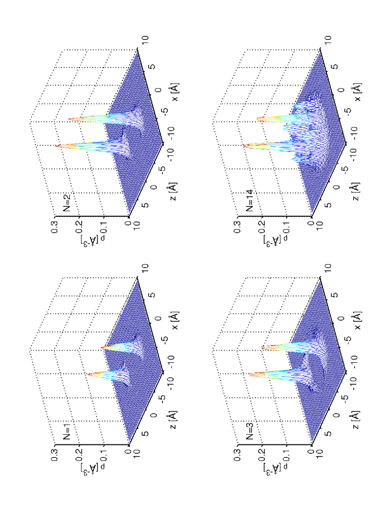
Figure 2: Cuts of the helium density in the BF frame along the $y=0$ plane, for $N=1,2,3,14$. The two dominant peaks at $z=\pm 3.7$ Å each correspond to a single helium atom situated on the molecule $C_{6}$-axis, above and below the benzene plane.

These cuts are taken along a plane perpendicular to the benzene molecular plane, bisecting two parallel carbon-carbon bonds. All structural quantities given here are obtained from DMC using the descendant weighting procedure described in Sec. III.2, and are thus sampled from the exact ground-state density distribution $\phi_{0}^{2}$. For $N=1,2$, the helium density along the benzene $C_{6}$-axis has two maxima at $z=\pm 3.7$ Å, which is in good agreement with the corresponding value of $z=\pm 3.5$ Å inferred from spectroscopic measurements.Beck et al. (1979) The positions of these two density maxima remain unchanged as $N$ increases to 14. As evident in Fig. 2, the local density near the benzene impurity is highly structured, which is reflective of the strong anisotropy in the helium-benzene interaction potential. We note that neglecting the rotational terms in the benzene kinetic energy, Eq. (2), leads to a considerably more strongly peaked helium density distribution in the BF frame.Patel et al. (2002)

V.2 Excited states

We have calculated helium vibrational excited-state energies for the ⁴He_N-benzene system, using the POITSE methodology described in Sec. III.3. For the $N=1$ dimer, each individual excitation operator $\hat{A}_{lm}^{\dagger}$ gives a well-defined excitation, by which we mean a spectral function $\kappa(E)$ consisting of a single, sharp peak. This indicates that the trial excited state given by $\hat{A}_{lm}^{\dagger}\Psi_{T}$ is a good approximation to a true eigenstate of the system, having non-negligible overlap with only a single $\phi_{n}$. The various spectral functions are superimposed and shown in the upper panel of Fig. 3.

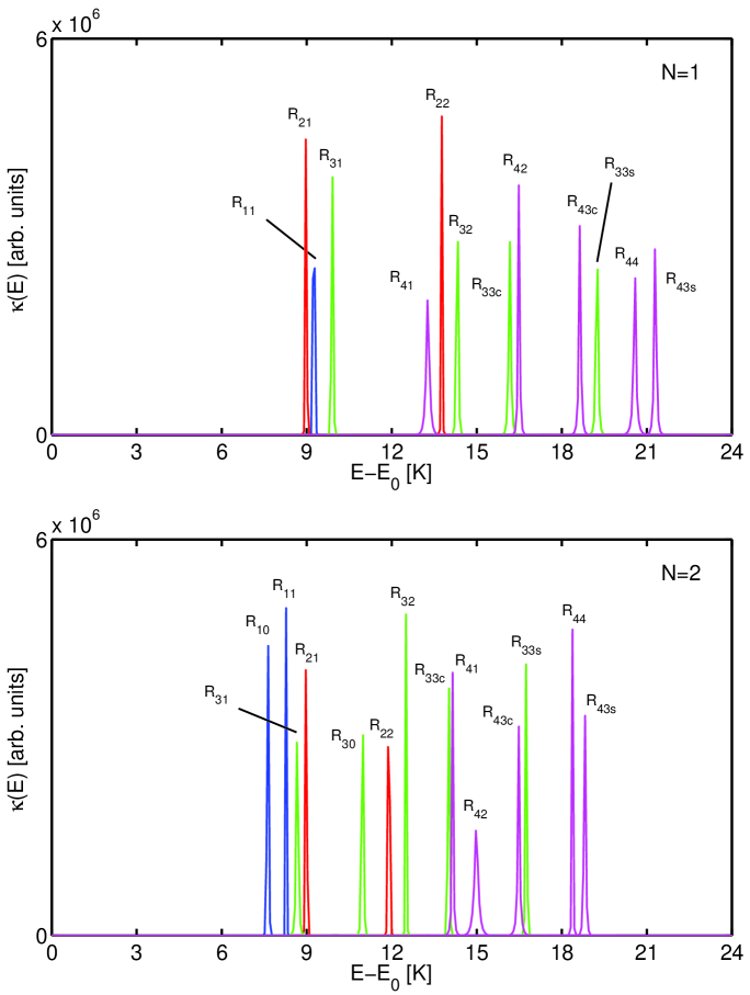
Figure 3: POITSE spectrum for $N=1$ (upper panel) and $N=2$ (lower panel). The peaks are color-coded according to excitations derived from excitation operators of different $l$ (Table 2).

For $N=1$, these helium vibrational modes begin at $\sim 9$ K above the ground state. Below this onset, we would expect to see excitations involving rotational motion of the much heavier benzene impurity, which lie in the spectral range studied experimentally by Beck et al.Beck et al. (1979) The excitations shown in the upper panel of Fig. 3 can be grouped into pairs split by $\sim 0.6-2.3$ K, corresponding to states generated by the application of pairs of projectors which are symmetric and antisymmetric with respect to reflection about the benzene molecular plane (Table 2). Since the $N=1$ projectors used here all give well-defined excitations, we conclude that these states represent symmetric and antisymmetric tunneling pairs. We are not able to extract the lowest tunneling excitation given by the application of the $R_{10}=z$ operator. This is likely due to its energy being too close to the ground state $E_{0}$, and thus its DMC imaginary-time evolution is too slow relative to the DMC propagation times used for the excited-state calculations here. These tunneling energetics are comparable to those obtained from basis set calculations of the 2,3-dimethylnaphthalene$\cdot$He complex by Bach et al.Bach et al. (1997) These authors found tunneling excitations associated with the motion of the single complexed helium atom from one side of the planar aromatic moiety to the other side, with splittings ranging from $<0.0014$ K for strongly localized states, and up to $4.6$ K for highly delocalized states.

The Bose-symmetrized versions of the excitation operators used for $N=1$ give a similar set of well-defined excitations for $N=2$, which are shown in the lower panel of Fig. 3. Thus, we conclude that these represent single-particle-like excitations, which is reasonable since the two helium atoms reside in the two equivalent global minima along the benzene $C_{6}$-axis, and are well-separated by the benzene plane. In general, the $N=2$ excitation energies $E-E_{0}$ tend to be slightly lower than those for $N=1$, with the onset of helium vibrational excitations beginning at $\sim 7.5$ K for $N=2$, as compared to $\sim 9$ K for $N=1$. Unlike the situation for $N=1$, the addition of a second particle now allows for a well-defined excitation of $A_{2u}$ symmetry at 7.63(4) K, obtained from the $R_{10}=z$ operator. We note that neglecting the rotational terms in the benzene kinetic energy, Eq. (2), alters the energy spectrum significantly.Huang et al. (2002)

With the two global minima occupied at $N=2$, an additional third helium atom must be delocalized over the twelve secondary minima, due to the effect of helium-helium repulsions. Thus, the character of the excited states is expected to change dramatically as the number of helium atoms increase from $N=2$ to $N=3$. This is evident in the POITSE calculations, where the projectors that give well-defined excitations for $N=1,2$ (Fig. 3) now give multiple peaks for $N=3$, shown in the upper panel of Fig. 4.

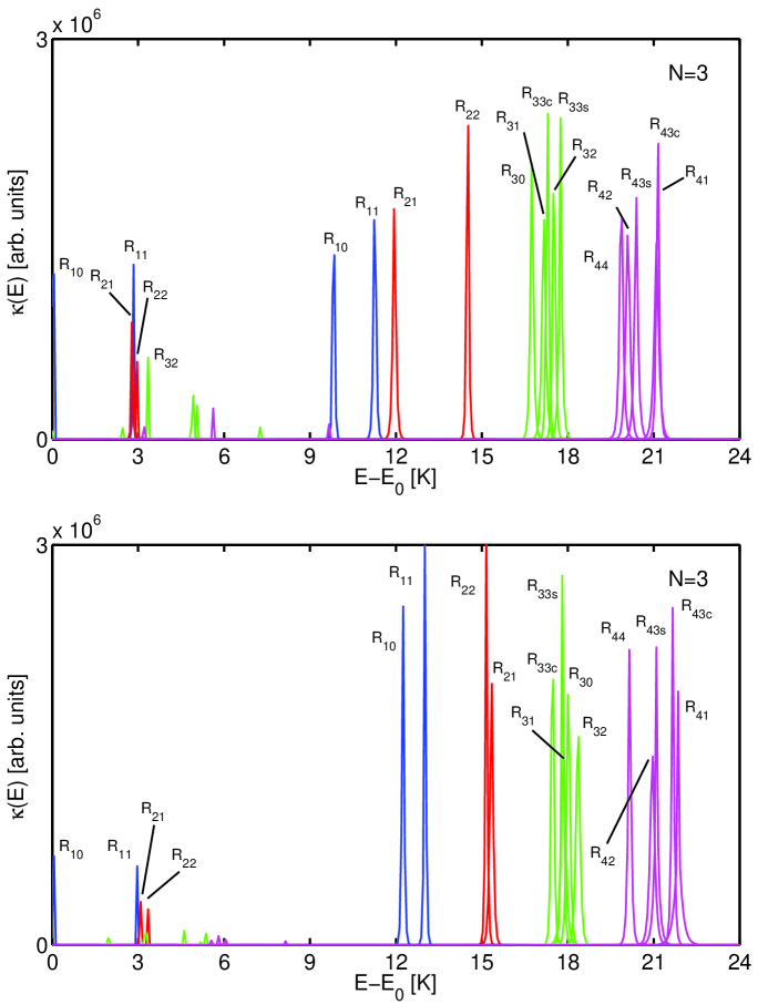
Figure 4: POITSE spectrum for $N=3$, deriving from $\hat{A}^{\dagger}$-type projectors (upper panel) and $\hat{B}^{\dagger}$-type projectors (lower panel). The peaks are color-coded according to excitations derived from excitation operators of different $l$ (Table 2).

This indicates that the starting excited state ansatz generated by $\hat{A}_{lm}^{\dagger}\Psi_{T}$ now has appreciable overlap with more than one eigenstate. Since the POITSE methodology does not provide information on excited-state wave functions, interpretation of the $N=3$ excitations is now less straightforward. Additional insight can be gained by making modifications to the projectors. The most noticeable new feature of the $N=3$ spectrum here is the appearance of lower-energy states at $<9$ K. Since the two atoms situated near the global potential minima experience a very different local environment from the third atom that is delocalized over the twelve secondary minima, the question then arises as to whether one can ascribe any of the excitations to motion localized near the global potential minima alone. We explore this here by defining a set of weighted “local” excitation operators

$$\hat{B}_{lm}^{\dagger}(\mathcal{R})=\sum_{j=1}^{N}\frac{R_{lm}(\mathbf{r}_{j})}{\prod_{\gamma\neq\gamma^{\prime}}\xi_{\gamma}(\mathbf{r}_{j})},$$ (52)

where the product in the denominator is taken over all localization factors that are not centered near the global minima. Application of these $\hat{B}^{\dagger}$-type projectors on $\Psi_{T}$ gives the following local excited-state ansatz:

$$\Psi =\hat{B}^{\dagger}_{lm}\Psi_{T}$$ (53)

$$=\sum_{j=1}^{N}\xi(\mathbf{r}_{1})\xi(\mathbf{r}_{2})\ldots\frac{R_{lm}(\mathbf{r}_{j})\xi(\mathbf{r}_{j})}{\prod_{\gamma\neq\gamma^{\prime}}\xi_{\gamma}(\mathbf{r}_{j})}\ldots\xi(\mathbf{r}_{N})\prod_{i<j}^{N}\chi(r_{ij}).$$ (54)

By substituting Eq. (43) for $\xi(\mathbf{r}_{j})$ in Eq. (54) above, it can be seen that the action of $\hat{B}^{\dagger}_{lm}$ is to place an atom in an excited single-particle state that is spatially localized near the set of sites $\{\mathbf{s}_{\gamma^{\prime}}\}$ only, i.e. near the two global potential minima. These operators are local in the sense that they act primarily on helium density near these two minima, while still maintaining spatial and Bose permutation symmetry. In contrast, by comparison with Eq. (51), we see that the $\hat{A}^{\dagger}$ operators are global operators, acting on all sites.

The spectrum for $N=3$ generated by the set of $\hat{B}^{\dagger}$-type projectors is shown in the lower panel of Fig. 4. Compared to the spectrum derived from $\hat{A}^{\dagger}$-type projectors (upper panel of Fig. 4), the spectral weight of lower-energy states are now reduced relative to the higher-energy excitations. A few low-energy features at $<9$ K persist, in particular the $R_{10}$ and $R_{11}$ excitations, albeit with reduced weights. Thus we conclude that the higher-energy excitations above $\sim 9$ K are associated with states that are spatially localized near the global minimum of the interaction potential, while the excitations below this range are associated with collective helium states of a more delocalized nature. For each set of states generated by a projector of given $l$, corresponding states of different $m$ are clustered more closely together than in the $N=1,2$ spectra, with each cluster of different $l$ spaced $\sim 3$ K apart.

As $N$ increases from 3 to 14, the ground-state DMC calculations reveal that the two global minima and twelve secondary minima are completely occupied (see Sec. V.1 and Fig. 2). An unambiguous determination of excited state energies at this size becomes more difficult due to the increase in Monte Carlo noise. However, certain qualitative features remain apparent. The upper panel of Fig. 5

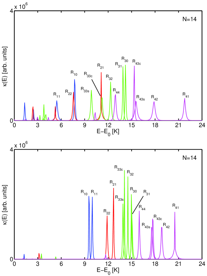
Figure 5: POITSE spectrum for $N=14$, deriving from $\hat{A}^{\dagger}$-type projectors (upper panel) and $\hat{B}^{\dagger}$-type projectors (lower panel). The peaks are color-coded according to excitations derived from excitation operators of different $l$ (Table 2).

shows the POITSE excitation spectrum for $N=14$, derived from the $\hat{A}^{\dagger}$-type global projectors. These projectors generate trial excited states which overlap with multiple eigenstates, and the resulting spectrum for a given projector has multiple peaks at both low and high energies. This problem, along with the accompanying increase in statistical noise in going to $N=14$, gives a spectrum which is not fully converged in the sense that the peak widths are broader and the peak positions shift (by up to $\sim 3$ K) with additional sampling. Nevertheless, we can again achieve qualitative insight by comparing with spectra derived from the localized $\hat{B}^{\dagger}$-type projectors. The lower panel of Fig. 5 shows the spectrum derived from the $\hat{B}^{\dagger}$-type projectors. There, the spectral weights of low-energy excitations ($<9$ K) are again significantly reduced just as the $N=3$ case, and each projector $\hat{B}_{lm}$ gives a $\kappa(E)$ consisting of a single dominant peak. While the higher-energy $l=4$ excitations are probably still not fully converged, the $l=1-3$ peaks do not shift much (less than $0.5$ K) with additional sampling, and appear to be converged. Thus the qualitative trends can be clearly established. Similar to the $N=3$ case, the localized projectors give rise to a set of higher-energy excitations, except red-shifted by $\sim 3$ K in comparison to the $N=3$ energies. For each $l$, states of different $m$ are now clustered together as was also the case for $N=3$ (Fig. 4). These states represent the localized vibrational motion of a single helium atom near the global potential minima, and appear to be associated with the localized helium density found in the path integral calculations of Ref. Kwon and Whaley, 2001. The lower-energy excitations, on the other hand, are associated with collective vibrations delocalized around the periphery of the molecule surface.

VI Summary Discussion and Implications for larger molecules

We have computed ground-state energies and structures for small ⁴He_N-benzene clusters, where $N=1,2,3,14$. For these sizes, the effect of the strong and highly anisotropic helium-benzene interaction potential gives rise to a very structured helium density distribution in the BF frame. In particular, a single helium atom is well-localized at each of the two equivalent global potential minima, above and below the benzene surface. We find a set of collective helium excitations with energies of up to $\sim 23$ K above the ground state. Among these excitations, the higher-energy states ($>9$ K) can be characterized as a localized excitation deriving from the helium density near the global potential minima, i.e. adsorbed on the molecular nanosurface. The existence of these localized modes is consistent with the localization of a single “dead” helium atom seen in Ref. Kwon and Whaley, 2001. Helium excitations of lower energies were also obtained, which correspond to collective vibrations of helium atoms delocalized over equivalent sites of lower binding energy, situated near the edges of the benzene surface. Both localized and delocalized excitations can also be further classified by their symmetry with respect to the $D_{6h}(M)$ group.

The energetic range of these helium excitations is similar to that observed experimentally as vibronic structure in the mass-selective excitation spectra of planar aromatic molecules in small helium clusters ($N\leq 16$).Even et al. (2000, 2001) It is also similar to the energetic range of the peaks observed in the phonon wings of vibronic spectra of planar aromatic molecules in large helium droplets.Hartmann et al. (1998, 2001); Lindinger et al. (2001); Hartmann et al. (2002) Thus, these calculations provide support for the picture of helium atoms adsorbed and vibrating on the molecule surface, with the specific details of the helium motions being determined by the geometry of the surface. In particular, the close relationship between the anisotropy of the molecule-helium interaction and the nature and energetic range of the excitations seen here for benzene implies that these molecule-induced vibrational modes will be very sensitive to the identity of the molecule, possibly even to the extent of providing a spectral “fingerprint” of complex polyaromatic species. Since these calculations have less than one solvation shell of helium surrounding the molecule, they are directly relevant to the recent experimental observations for small cluster sizes.Even et al. (2000, 2001) Moreover, the analysis of the excitations has been made in terms of single-particle type excitation operators acting on the many-body ground state, and is thus applicable to any number of solvating helium atoms. The fact that the localized excitation associated with the most strongly bound helium density at the global minimum persists in the largest cluster studied here ($N=14$), together with the previous identification of localization at that site in larger helium clusters,Kwon and Whaley (2001) indicates that these localized excitations will also be present in much larger helium droplets. For the ⁴He_N-benzene system here we have examined the limit of a single helium adsorbed atom on a single site given by the benzene nanosurface. But given the energetics that we find here, in a more general sense this class of surface-adsorbed vibrations are very likely to be responsible for the structure seen in the phonon wing sideband in experiments using helium droplets.Hartmann et al. (2002)

A detailed analysis of the experimental phonon wing data clearly requires molecule-specific calculations with accurate potential surfaces. For example, the region of spatial confinement for an adsorbed helium atom near the global potential minimum is smaller in benzene than in the larger polyaromatic molecules studied experimentally with small numbers of helium atoms in Ref. Even et al., 2001. In a general context, the present results are very encouraging in that they show that the diffusion Monte-Carlo based methodologies can be used to systematically study these excitations as a function of the number of helium atoms, provided that realistic molecule-helium interaction potentials are available. We emphasize here that a quantitative analysis, both for the small cluster vibronic excitations and for the phonon wing structure in electronic absorption spectra, will require detailed knowledge of the molecule-helium interaction potential in both ground and electronically excited states.

Less obvious than the relation to phonon wing structure is whether the excitations of the type studied here are responsible for the splittings on the order of $\sim 1$ K in the zero-phonon line, which were observed for some large organic impurity molecules in large helium droplets. This zero-phonon line splitting has been experimentally studied in detail for tetracene,Hartmann et al. (2001); Lindinger et al. (2001) and for indole derivatives.Lindinger et al. (2001) In both experimental studies rotational fine structure has been ruled out as being responsible and several different interpretations have been advanced. For tetracene, a molecule possessing a plane of mirror symmetry, it has been suggested that either two inequivalent helium binding sites exist, possibly due to an inhomogeneous solvation environment, or that some kind of two-particle tunneling is manifested.Hartmann et al. (2001) For indole derivatives, molecules possessing aromatic rings but no mirror symmetry and not usually completely planar, the theoretical evidence of localized helium atoms at aromatic rings in larger, superfluid, helium clustersKwon and Whaley (2001) has been used to propose models of helium atoms similarly localized on either side of the aromatic portion of the molecule.Lindinger et al. (2001)

The ⁴He_N-benzene calculations reported here show low-lying excited states ($\leq 9$ K) for the larger clusters, $N=3,14$. Furthermore, the spectral weights of these low-lying states do decrease significantly relative to the higher-energy states when the local $\hat{B}^{\dagger}$-type operators are applied. This shows that the low-energy spectral features we observe the our calculations are due to vibrational motion of helium located near the periphery of the benzene surface, since the $\hat{B}^{\dagger}$-type operators specifically de-emphasize states that are not strongly localized near the global potential minima. In contrast to the higher-lying localized states, it is more difficult to say whether these low-energy states would remain low-energy with increasing $N$, since addition of more helium atoms would be expected to significantly change the local details of the helium wave function in these edge regions around the molecule. Thus, it is also more difficult to conclusively claim that these low-energy delocalized modes are responsible for the experimentally observed splittings in the zero-phonon lines.

However, with aromatic molecules of lower overall symmetry like the indole derivatives, it appears reasonable that the effective potential on opposite sides of the aromatic ring may differ, due to the effect of non-symmetric, three-dimensional side chains, resulting in slightly different localized helium densities on either side of the aromatic ring, as proposed in Ref. Lindinger et al., 2001. This suggests that an alternative approach to interpret the splitting of zero-phonon lines in experiments would be in the context of impurity spectra in solids, where the impurity molecule can be trapped in structurally inequivalent trapping sites, giving rise to small differences in the spectral shifts of the electronic origin.Rebane (1970) Quantitative analysis of this kind would also require determination of accurate helium solvation densities around the molecule.

In extrapolating conclusions made from small cluster studies, whether theoretical or experimental, to explain experimental observations made in large droplets, the key point to consider is whether the localization induced by the helium-aromatic molecule interaction is sufficiently strong such that the localized helium excitations characterized here persist with increasing $N$. As the number of helium atoms increases, collective compressional and surface modes of the droplet are expected to develop, and the coupling to these modes are manifest in the phonon-wing sideband in electronic spectra measured in large droplets.Hartmann et al. (1996) The path integral results for benzene in ⁴He₃₉ provide evidence that the single localized helium atom located on either side of the molecule near the global potential minimum does indeed retain its localized identity in large clusters.Kwon and Whaley (2001) This provides a strong argument for the persistence of the single-particle-like localized states whose excitations have been characterized here for smaller clusters ($N\leq 14$). An important task for future work is to understand how the discrete spectra for larger polyaromatics vary with the number of helium atoms when this is still less than a solvation shell,Even et al. (2001) as well as what happens to these excitations in much larger helium clusters. A theoretical prerequisite for study of all these excitations is now the development of accurate trial functions for these very anisotropic aromatic systems at larger numbers of helium atoms ($N>14$). This will then allow analysis of the transition from localized to collective helium vibrations, as well as identification of any persistent localized modes that may exist at an aromatic molecular nanosubstrate.

VII Acknowledgments

We acknowledge financial support from the National Science Foundation under grants CHE-9616615 and CHE-0107541. Computational support was provided in part by the National Partnership for Advanced Computational Infrastructure (NPACI) at the San Diego Supercomputer Center. KBW thanks the Miller Institute for Basic Research in Science for a Miller Research Professorship for 2002–2003.

References

- Toennies et al. (2001) J. P. Toennies, A. F. Vilesov, and K. B. Whaley, Phys. Today 54, 31 (2001).
- (2) For recent developments, see the articles under the Special Topic Helium nanodroplets: a novel medium for chemistry and physics, edited by R. E. Miller and K. B. Whaley, in J. Chem. Phys. 115, 10065–10281 (2001).
- Hartmann et al. (1996) M. Hartmann, F. Mielke, J. P. Toennies, A. F. Vilesov, and G. Benedek, Phys. Rev. Lett. 76, 4560 (1996).
- Grebenev et al. (2000) S. Grebenev, M. Hartmann, A. Lindinger, N. Pörtner, B. Sartakov, J. P. Toennies, and A. F. Vilesov, Physica B 280, 65 (2000).
- Stienkemeier and Vilesov (2001) F. Stienkemeier and A. F. Vilesov, J. Chem. Phys. 115, 10119 (2001).
- Hartmann et al. (1998) M. Hartmann, A. Lindinger, J. P. Toennies, and A. F. Vilesov, Chem. Phys. 239, 139 (1998).
- Hartmann et al. (2001) M. Hartmann, A. Lindinger, J. P. Toennies, and A. F. Vilesov, J. Phys. Chem. A 105, 6369 (2001).
- Lindinger et al. (2001) A. Lindinger, E. Lugovoj, J. P. Toennies, and A. F. Vilesov, Z. Phys. Chem. 215, 401 (2001).
- Hartmann et al. (2002) M. Hartmann, A. Lindinger, J. P. Toennies, and A. F. Vilesov, Phys. Chem. Chem. Phys. 4, 4839 (2002).
- Even et al. (2000) U. Even, J. Jortner, D. Noy, and N. Lavie, J. Chem. Phys. 112, 8068 (2000).
- Even et al. (2001) U. Even, I. Al-Hroub, and J. Jortner, J. Chem. Phys. 115, 2069 (2001).
- Bretz et al. (1973) M. Bretz, J. G. Dash, D. C. Hickernell, E. O. McLean, and O. E. Vilches, Phys. Rev. A 8, 1589 (1973).
- Shirron and Mochel (1991) P. J. Shirron and J. M. Mochel, Phys. Rev. Lett. 67, 1118 (1991).
- Greywall and Busch (1991) D. S. Greywall and P. A. Busch, Phys. Rev. Lett. 67, 3535 (1991).
- Zimmerli et al. (1992) G. Zimmerli, G. Mistura, and M. H. W. Chan, Phys. Rev. Lett. 68, 60 (1992).
- Adams and Pant (1992) P. W. Adams and V. Pant, Phys. Rev. Lett. 68, 2350 (1992).
- Clements et al. (1993) B. E. Clements, J. L. Epstein, E. Krotscheck, and M. Saarela, Phys. Rev. B 48, 7450 (1993).
- Wagner and Ceperley (1994) M. Wagner and D. M. Ceperley, J. Low Temp. Phys. 94, 185 (1994).
- Dalfovo et al. (1995) F. Dalfovo, A. Lastri, L. Pricaupenko, S. Stringari, and J. Treiner, Phys. Rev. B 52, 1193 (1995).
- Csáthy et al. (1998) G. A. Csáthy, D. Tulimieri, J. Yoon, and M. H. W. Chan, Phys. Rev. Lett. 80, 4482 (1998).
- Nyéki et al. (1998) J. Nyéki, R. Ray, B. Cowan, and J. Saunders, Phys. Rev. Lett. 81, 152 (1998).
- Pierce and Manousakis (1999) M. E. Pierce and E. Manousakis, Phys. Rev. Lett. 83, 5314 (1999).
- Lauter et al. (1992) H. J. Lauter, H. Godfrin, and P. Leiderer, J. Low Temp. Phys. 87, 425 (1992).
- Clements et al. (1996) B. E. Clements, H. Godfrin, E. Krotscheck, H. J. Lauter, P. Leiderer, V. Passiouk, and C. J. Tymczak, Phys. Rev. B 53, 12242 (1996).
- Kwon and Whaley (2001) Y. Kwon and K. B. Whaley, J. Chem. Phys. 114, 3163 (2001).
- Krishna and Whaley (1990) M. V. R. Krishna and K. B. Whaley, J. Chem. Phys. 93, 746 (1990).
- Chin and Krotscheck (1992) S. A. Chin and E. Krotscheck, Phys. Rev. B 45, 852 (1992).
- Chin and Krotscheck (1995) S. A. Chin and E. Krotscheck, Phys. Rev. Lett. 74, 1143 (1995).
- Bach et al. (1997) A. Bach, S. Leutwyler, D. Sabo, and Z. Bačić, J. Chem. Phys. 107, 8781 (1997).
- Anderson et al. (2000) S. M. Anderson, J. Ka, P. M. Felker, and D. Neuhauser, Chem. Phys. Lett. 328, 516 (2000).
- Heidenreich et al. (2001) A. Heidenreich, U. Even, and J. Jortner, J. Chem. Phys. 115, 10175 (2001).
- Leutwyler and Jortner (1987) S. Leutwyler and J. Jortner, J. Phys. Chem. 91, 5558 (1987).
- Blume et al. (1997) D. Blume, M. Lewerenz, P. Niyaz, and K. B. Whaley, Phys. Rev. E 55, 3664 (1997).
- Aziz et al. (1987) R. A. Aziz, F. R. W. McCourt, and C. C. K. Wong, Mol. Phys. 61, 1487 (1987).
- Hobza et al. (1992) P. Hobza, O. Bludský, H. L. Selzle, and E. W. Schlag, J. Chem. Phys. 97, 335 (1992).
- Bunker and Jensen (1998) P. R. Bunker and P. Jensen, Molecular Symmetry and Spectroscopy (NRC Research Press, Ottawa, 1998), 2nd ed.
- Hammond et al. (1994) B. L. Hammond, W. A. Lester, Jr., and P. J. Reynolds, Monte Carlo Methods in Ab Initio Quantum Chemistry (World Scientific, Singapore, 1994).
- Viel et al. (2002) A. Viel, M. V. Patel, P. Niyaz, and K. B. Whaley, Comp. Phys. Com. 145, 24 (2002).
- Liu et al. (1974) K. S. Liu, M. H. Kalos, and G. V. Chester, Phys. Rev. A 10, 303 (1974).
- Blume (1998) D. Blume, Ph.D. thesis, University of Göttingen (1998).
- Huang et al. (2002) P. Huang, A. Viel, and K. B. Whaley, in Recent Advances in Quantum Monte Carlo Methods, Part II, edited by W. A. Lester, Jr., S. M. Rothstein, and S. Tanaka (World Scientific, Singapore, 2002), vol. 2 of Recent Advances in Computational Chemistry, p. 111, eprint physics/0203012.
- Jarrell and Gubernatis (1996) M. Jarrell and J. E. Gubernatis, Phys. Rep. 269, 133 (1996).
- Bryan (1990) R. K. Bryan, Eur. Biophys. J. 18, 165 (1990).
- Gubernatis et al. (1991) J. E. Gubernatis, M. Jarrell, R. N. Silver, and D. S. Sivia, Phys. Rev. B 44, 6011 (1991).
- Sivia (1996) D. S. Sivia, Data analysis: a Bayesian tutorial (Clarendon Press, Oxford, 1996).
- McMillan (1965) W. L. McMillan, Phys. Rev. 138, A442 (1965).
- Mushinski and Nightingale (1994) A. Mushinski and M. P. Nightingale, J. Chem. Phys. 101, 8831 (1994).
- Reatto (1979) L. Reatto, Nucl. Phys. A 328, 253 (1979).
- Vitiello et al. (1988) S. Vitiello, K. Runge, and M. H. Kalos, Phys. Rev. Lett. 60, 1970 (1988).
- McMahon et al. (1993) M. A. McMahon, R. N. Barnett, and K. B. Whaley, J. Chem. Phys. 99, 8816 (1993).
- Cheng et al. (1996) E. Cheng, M. A. McMahon, and K. B. Whaley, J. Chem. Phys. 104, 2669 (1996).
- Beck et al. (1979) S. M. Beck, M. G. Liverman, D. L. Monts, and R. E. Smalley, J. Chem. Phys. 70, 232 (1979).
- Patel et al. (2002) M. V. Patel, A. Viel, F. Paesani, P. Huang, and K. B. Whaley, J. Chem. Phys. (2002), submitted.
- Rebane (1970) K. K. Rebane, Impurity spectra of solids (Plenum Press, New York, 1970).