Accurate and concise atomic CI via generalization of analytic Laguerre type orbitals and examples of ab-initio error estimation for excited states

Abstract

We propose simple analytic, non-orthogonal but selectively orthogonalizable, generalized Laguerre type atomic orbitals, providing clear physical interpretation and near equivalent accuracy with numerical multi-configuration self-consistent field, to atomic configuration interaction calculations. By analyzing the general Eckart theorem we use their simple interpretation, via a thorough investigation in orbital space, to estimate, for the first time (the exact value being, or considered, unknown), an ab-initio energy uncertainty, i.e. proximity to the exact energy, for several excited atomic states known to have the danger to suffer from variational collapse.

I Outline

The purpose of this paper is threefold. (i) First is to show that, in variational ab-initio atomic configuration interaction (CI) calculations (for the ground or excited states), by varying the extent and the node positions of the (analytic) orbital radial functions, it is possible to achieve nearly numerical multi-configuration self-consistent field (NMCSCF) accuracy. (This means that the resulting analytic orbitals, similar to NMCSCF orbitals, are few, concise, clearly interpretable and with rich physical content). (ii) The second purpose is to analyze and clarify an extension of the Eckart theorem for excited states (c.f. Appendix). (iii) The third is to demonstrate that, (with the help of these, at least, orbitals), within the general Eckart theorem, it is possible to obtain an ab-initio estimate of the proximity to the (supposedly unknown) exact energy, at least in some special cases of CI expansions. Consequently it is possible, in these cases, that other outcomes (outside of the uncertainty error) be ab initio rejected without the need of external information.

II Introduction

(i) Among various configuration interaction (CI) methods for the calculation of the electronic structure of atoms, based on the variational principle, the NMCSCF is very efficient and accurate because it describes the electronic state with few simple orbitals, rich in physical meaning, whereas other methods are based on large basis sets which complicate the description. It would be interesting to invent analytic orbitals similar to NMCSCF, thus describing the state in an equally simple and concise way, with comparable accuracy. We have invented such analytic semiorthogonal basis functions, which very satisfactorily approximate the NMCSCF orbitals: The central idea is to adopt the usual Laguerre orbitals and start moving variationally the nodes and the extent of their radial functions, until minimization of the energy. Eventually the resulting orbitals are similar and of comparable accuracy with NMCSCF. Nevertheless, since NMCSCF is numerical, it leads to an energy minimum, indifferently global or local, usually the widest (which is sometimes misinterpreted [scffail_b] ; [scffail_m] ) and other energy minima cannot be easily located, which may describe the state in a simpler way, i.e., with a smaller contribution of the higher order terms in the CI expansion. For this reason, by looking at only the widest minimum, the quality of the approximation to the exact eigenfunction cannot be ab-initio estimated. However, since our orbitals are analytic, all (finite in number) energy minima can be located, at least in principle, and because of the simplicity, and of the immediate recognizability of the physical content of the orbitals, the most representative description of the CI expansion can be chosen, therefore a measure of the quality of our approximation to the exact solution can be ab-initio estimated (without using other external information) via the correction introduced by the general Eckart theorem (c.f. Appendix). The analyticity of the orbitals allows also the flexibility to have orthogonal occupied orbitals and non-orthogonal some virtual correlation orbitals, thus accelerating the convergence of the CI expansion.

(ii) On the other hand, for some excited states, like He 1s2s ${}^{1}S$, Mg 3s4s ${}^{1}S$ etc [18] , the variational calculation may collapse to a lower lying than the exact state, which is wrong, but allowed by the general Eckart theorem for excited states (c.f. Appendix). It would be interesting, if possible, to invent an ab-intio (without other external information) way to reject such wrong outcomes and to variationally bracket the unknown exact energy level within some known digits of certainty. To this end we propose a method, feasible with the presented orbitals, valid under certain conditions, and demonstrate it in several cases with two or three electrons. We also discuss the extent of its feasibility.

III Part I. Atomic CI via generalization of Laguerre type orbitals

We propose a generalization of Laguerre type orbitals to the form $\langle\textbf{r}|n,l,m\rangle$ $=$ $A_{n,l,m}$ $L_{n,l}(\{g\},r,z_{n,l},b_{n,l},q_{n,l})$ $Y_{l,m}(\theta,\phi)$, where $A_{n,l,m}$ is a normalization constant and $Y_{l,m}(\theta,\phi)$ are spherical harmonics. The generalized Laguerre type functions (GLTOs) are (in a.u.)

$$L_{n,l}(\{g\},r,z_{n,l},b_{n,l},q_{n,l})=\sum\limits_{k{\rm=0}}^{n-l-1}{{\rm c}_{k}}(n,l,z_{n,l})g_{k}(n,l,\{z_{i,l},b_{i,l},q_{i,l}\}_{i=1}^{n})r^{l+k}\exp(-z_{n,l}r/n)$$

$$+b_{n,l}\exp(-q_{n,l}z_{n,l}r/n)\delta_{l,0}$$ (1)

where $g_{n-l-1}(n,l,\{z_{i,l},b_{i,l},q_{i,l}\}_{i=1}^{n})$ $=1$ (about the rest of the $g_{k}$ factors we extensively discuss below) and $c_{k}$ are the usual associated Laguerre polynomial coefficients. The parameters $z_{n,l}$, $b_{n,l}$, $q_{n,l}$ are determined from the (non-linear variational) minimization [10] of the desired root of the secular equation (see below equation (5)). The $z_{n,l}$ parameters are effective nuclear charges and determine the radial extent of the orbitals. Since $z_{n,l}$ differ from orbital to orbital, these orbitals are, in general, non-orthogonal. The addition of the last term of equation (1) just modifies the radial part of $s$-orbitals, since 1s cannot be modified by any $g_{k}$ factor.

Then, a normalized CI wave function is formed out of Slater determinants (composed of the proposed orbitals), whose node positions and radial extent are optimized variationally through non-linear multidimensional minimization of the total energy. We present a selective intrinsic orthogonalization formalism to any lower $n$,$l$ orbital of either the ground, or a desired excited state, thus preserving the orbital characteristics. The rest of the orbitals remain non-orthogonal (e.g., see table 1 below). We first find (and use) a main wave function in the dominant part of the active space (called ‘main’), well representing the state under consideration [e.g., for He, in the active space of $2s$, $2p$, $3s$, $3p$, the four ${}^{1}P^{o}$ roots have the following ‘main’ wave functions: ($2s2p$), ($2s3p\pm 3s2p$) and ($3s3p$)], and then we add angular and radial correlation [2] , simulating cusp conditions. The method is tested against several known cases.

Thus, given the atom with nuclear charge $Z_{nuc}$, and $N$ electrons, with space and spin coordinates $\textbf{r}_{1}s_{1},...,\textbf{r}_{N}s_{N}$, as well as the symmetry and the electron occupancy, the desired $N-$electron normalized wave function, consisting of $N_{c}$ (predetermined) configurations, out of $N_{d}$ Slater determinants, is

$$\begin{array}[]{l}\Psi({\bf r}_{1}s_{1},...,{\bf r}_{N}s_{N})=\sum\limits_{p=1}^{N_{c}}{c_{p}\Gamma_{p}}({\bf r}_{1}s_{1},...,{\bf r}_{N}s_{N});\\ \left|\Psi\right|^{2}=1;\Gamma_{p}=\sum\limits_{i=1}^{N_{d}}{f_{ip}}D_{i}\\ \end{array}$$ (4)

where the linear parameters $c_{p}$ are determined from a desired (usually the lowest) root of the secular equation

$$\det\left[\left(\sum\limits_{a,b=1}^{N_{d}}{f_{ap}f_{bq}}\left\langle{D_{a}}\right|H-E\left|{D_{b}}\right\rangle\right)_{p,q}\right]_{N_{c}\times N_{c}}=0$$ (5)

which is solved by the strategy of p. 455 of “Numerical Recipes” [6] . Here $E$ is the total energy, the Hamiltonian matrix elements are calculated by the method of p. 66 of McWeeny [7] , where

$$H =-\frac{1}{2}\sum\limits_{i=1}^{N}{(\nabla_{i}^{2}+\frac{{Z_{nuc}}}{{\left|{{\bf r}_{i}}\right|}}})+\sum\limits_{i>j}^{N}{\frac{1}{{\left|{{\bf r}_{i}-{\bf r}_{j}}\right|}}}$$ (6)

$$~{}\equiv\sum\limits_{i=1}^{N}h(i)+\sum\limits_{i>j}^{N}g(i,j);$$

the $D_{a}$ are all ($N_{d}$) (consistent with the desired electronic state) Slater determinants, formed out of $N_{orb}$ (predetermined), to be optimized, spinorbitals $a_{i}$, and $f_{ap}$ are all ($N_{d}\times N_{c}$) consistent corresponding coefficients, which we determine by implementing the ideas of Schaefer and Harris’s method [8] . The angular (and spin) part of the matrix elements in equation (5) we treat according to the method of chapter 6 of Tinkham [9] .

The adaptability of our orbitals to almost NMCSCF accuracy is due to the $g_{k}$-factors, which move, during the minimization process, the orbital nodes appropriately, by intrinsic orthogonalization among desired orbitals of the same [11] or of a different [5] state (an advantage of this method), by directly solving $\langle n_{i},l,m|n_{j},l,m\rangle$ $=$ $\delta_{i,j}$, $(i,j=1,...,N_{orb})$. For example, for the $1s$ and $2s$ orbitals, equation $\langle 1s|2s\rangle=0$ yields

$$g_{0}(2,s,\{z_{1s},z_{2s}\})={\frac{{\frac{6\,z_{2s}}{{{\left(2\,z_{1s}+z_{2s}\right)}^{4}}}}+{\frac{6\,b_{1s}\,z_{2s}}{{{\left(2\,q_{1s}\,z_{1s}+z_{2s}\right)}^{4}}}}-{\frac{b_{2s}}{{{\left(2\,z_{1s}+q_{2s}\,z_{2s}\right)}^{3}}}}-{\frac{b_{1s}\,b_{2s}}{{{\left(2\,q_{1s}\,z_{1s}+q_{2s}\,z_{2s}\right)}^{3}}}}}{{\frac{2}{{{\left(2\,z_{1s}+z_{2s}\right)}^{3}}}}+{\frac{2\,b_{1s}}{{{\left(2\,q_{1s}\,z_{1s}+z_{2s}\right)}^{3}}}}}}$$ (7)

and it is straightforward to derive the $g_{k}$-factors for $n=2,3,4,...$, $l=0,1,2,...,n-1$ and $k=1,...,n-l-2$ [1] ; [12] .

Thus these orbitals, after orthogonalization, are not linear combinations of each other, as in orther orthogonalization schemes, but maintain (c.f. equation (1) and figure (1) below) a clear physical interpretation for all $l=s,p,d,...$, enabling one, to choose reasonable (and to reject unreasonable) outcomes even by inspection.

Since the CI expansion may still contain non-orthogonal orbitals, we use the general non-orthogonal formalism of p. 66 of McWeeny [7] ,

$$\langle D_{a}|\sum\limits_{i=1}^{N}h(i)|D_{b}\rangle=$$

$$(D_{aa}D_{bb})^{-1/2}\sum\limits_{i,j=1}^{N}\langle a_{i}|h|b_{j}\rangle D_{ab}(a_{i}b_{j})$$ (8)

where $D_{ab}=det|\langle a_{1}|b_{1}\rangle\langle a_{2}|b_{2}\rangle...\langle a_{n}|b_{n}\rangle|$, $D_{ab}(a_{i}b_{j})$ denotes the cofactor of the element $\langle a_{i}|b_{j}\rangle$ in the determinant $D_{ab}$, and $D_{aa},D_{bb}$ are similar normalization factors; $a_{i}$, $b_{j}$ are the spinorbitals. Also,

$$\langle D_{a}|\sum\limits_{i>j}^{N}g(i,j)|D_{b}\rangle=$$

$$(D_{aa}D_{bb})^{-1/2}\sum\limits_{i>t}^{N}\sum\limits_{j>l}^{N}\langle a_{i}a_{t}|g|b_{j}b_{l}\rangle D_{ab}(a_{i}a_{t}b_{j}b_{l})$$ (9)

where $D_{ab}(a_{i}a_{t}b_{j}b_{l})$ is the cofactor of $D_{ab}$ defined by deleting the rows and columns containing $\langle a_{i}|b_{j}\rangle$ and $\langle a_{k}|b_{l}\rangle$ and attaching a factor $(-1)^{i+j+t+l}$ to the resultant minor. In principle, equations (8-9) can readily deal with Slater determinants for any large atom without leading to extra complexity, so that one need not adopt “limited non-orthogonality” in order to avoid complications.

We improve the N-electron wave function by incorporating radial and angular correlation so as to simulate the cusp conditions, either via orthogonalization to desired lower-$n$ orbitals, or via free non-orthogonality.

The contraction with the $l=0$ Slater type orbital (the last term of equation (1)), especially useful when there are outer electrons repelling the inner toward the nucleus, provides, in full CI, about 75% of the energy correction obtained if we freely doubled the (uncontracted) orbitals, while it substantially reduces the CI size; symbolically, $(E_{N}^{c}-E_{N}^{u})$ $\sim$ 75% $(E_{2N}^{u}-E_{N}^{u})$. Thus, for $Be$ $1s^{2}2s^{2}$ ${}^{1}S$, with 2 orbitals $1s$, $2s$ (1 configuration) we have (in $a.u.$) $E_{2}^{u}$ $=-14.5300$, $E_{2}^{c}$ $=-14.5723$, while with 4 orbitals $1s,1s^{\prime},2s,2s^{\prime}$ (20 configurations), $E_{4}^{u}=$ $-14.5893$; i.e., the contraction provides 71% of the corresponding (uncontracted) CI correction. Similarly, for the $H^{-}$ $1s^{2}$ ${}^{1}S$, with 4 orbitals of $1s$ type with 10 configurations we obtain $E_{4}^{u}=-0.51438$, $E_{4}^{c}$ $=-0.51445$, while 8 uncontracted $1s$ type orbitals with 36 configurations give $E_{8}^{u}=$ $-0.51448$, i.e., the contraction provides 74% of the corresponding free CI correction.

In addition, we performed several further tests:

1. For the $He$ ground state $1s^{2}$ ${}^{1}S$, if we use the uncontracted correlation orbitals of table (1) up to $4f^{\prime}$, we obtain (in $a.u.$) $E=-2.903104$, which is comparable with the NMCSCF value (up to $4f$) of $-2.903117$ [13] , the exact value being $-2.903724$ [14] .

2. For the $Li$ ground state $1s^{2}2s$ ${}^{2}S$, using uncontracted correlation orbitals up to $4f^{\prime}$, we obtain $E_{15}^{u}$ $=$ $-7.4767$ $a.u.$ [1] , which is comparable with the NMCSCF (up to $4f$) value of $-7.4762$ $a.u.$ [15] , while the exact value is $-7.4780$ $a.u.$ [16] .

3. For the $Li$ excited state $1s^{2}2p$ ${}^{2}P$, an example of straightforward slow CI convergence, using contracted correlation orbitals up to $4f$, we obtain $E_{13}^{c}=$ $-7.4080$ $a.u.$ [1] , comparable with the large CI (45 CI terms up to $5g$) value of $-7.4084$ $a.u.$ [wwa63] , while the experimental value is $-7.4099$ $a.u.$ [17] .

4. For the $C$ ground state $1s^{2}2s^{2}2p^{2}$ ${}^{3}P$, using uncontracted correlation orbitals up to $4f$, including $1s^{\prime}$, $2s^{\prime}$ and $2p^{\prime}$ (13 orbitals), by keeping 64 mostly significant configurations with 346 Slater determinants, we obtain $E=-37.78719$ $a.u.$, comparable with the value $E=-37.78695$ $a.u.$ obtained by large-scale NMCHF using up to $4f$ orbitals in active space [sun91] , and also with the value $E=-37.78885$ $a.u.$ obtained by large-scale MRCI using 145 Gaussion functions (17s11p6d5f4g2h) with $\thickapprox$ 1 500 000 configurations [mav99] . (With 90 orbitals and $\lessapprox$ 100 000 Slater determinants Sundholm and Olsen obtain $E=-37.79$ a.u.[sun91] , while Silverman [sil89] has obtained $E=-37.845$ $a.u.$ using 1/Z expansions).

5. Finally, for He $1s2s$ ${}^{1}S$, by implementing the Hylleraas-Undheim-MacDonald (HUM) theorem [11] with these orbitals, i.e. by optimizing the $2nd$ root of the secular equation (the $1st$ would provide the ground state within the same basis functions), we obtained for $1s^{2}+2s$: $E_{2}=-2.14261$ $a.u.;$ $1s^{2}+2s$ $(+1s^{\prime})$: $E_{2}=-2.14389$ $a.u.$ and $1s^{2}+2s$ $(+1s^{\prime})$ $+$ $2p$: $E_{2}=-2.14456$ $a.u.$. The corresponding NMCSCF values are $1s^{2}+2s$: $E=-2.14347$ $a.u.$ and $1s^{2}+2s+2p$: $E=-2.14380$ $a.u.$[13] .

We observe that our values are quite close to NMCSCF, so that our analytic orbitals and wavefunctions are quite trustable with nearly as small CI expansions as NMCSCF. I.e. variationally moving the nodes and the extent of the GLTOs they become quite similar to NMCSCF orbitals with the same rich and concise physical content.

IV Part II. An analysis of the general Eckart theorem

The general Eckart [5] theorem (GET) for excited states (c.f. Appendix), states that: The exact energy eigenvalue $E_{n}$, is a lower bound not of the calculated energy $E_{e}^{(n)}$ per se, but of the calculated augmented energy: $(E_{e}^{(n)}+\delta_{e}^{(n)})$ $\equiv$ [$E_{e}^{(n)}+\sum\limits_{i=1}^{n-1}{|\langle\psi_{i}|\Psi_{e}^{(n)}\rangle|^{2}(E_{n}-E_{i})}$ $\geq E_{n}$]. Here $\psi_{1}$, $\psi_{2}$, …, $\psi_{n}$, … are the exact eigenstates of the Hamiltonian $H$ with energies $E_{1}<E_{2}<...<E_{n}<...$, and $\Psi_{e}^{(n)}$ is the calculated normalized $(n-1)th$ excited state of the desired symmetry, with energy expectation value $E_{e}^{(n)}$.

Even if the exact $\psi_{i}$ were used, the augmentation $\delta_{e}^{(n)}$ would not be zero, for an approximate $\Psi_{e}^{(n)}$, so that, in trying to estimate the unknown $E_{n}$ via the minimization principle, by varying $\Psi_{e}^{(n)}$, the augmentation $\delta_{e}^{(n)}$ should be taken into account.

Since $E_{n}=E_{e}^{(n)}+\delta_{e}^{(n)}-\epsilon_{e}^{(n)}$ [equation (13) in Appendix], estimating $E_{n}$ requires minimization of both $\delta_{e}^{(n)}$ and $\epsilon_{e}^{(n)}$ $\equiv$ $\sum\limits_{k=n+1}^{\infty}{|\langle\psi_{k}|\Psi_{e}^{(n)}\rangle|^{2}(E_{k}-E_{n})}$, since both are unknown but positive. This can be achieved if $\Psi_{e}^{(n)}\approx\psi_{n}$. But then, since $\epsilon_{e}^{(n)}$ is positive and subtracted, we can have a rather conservative estimate of the error (the energy uncertainty of $E_{n}$) by $\delta_{e}^{(n)}$ [which we approximate by $\Delta_{e}^{(n)}\equiv\sum\limits_{i=1}^{n-1}{|\langle\Psi_{e}^{(i)}|\Psi_{e}^{(n)}\rangle|^{2}(E_{e}^{(n)}-E_{e}^{(i)})}$], provided that this dominates over the CI expansion truncation (convergence) error $\varepsilon$. Evidently, for a given $\Psi_{e}^{(n)}$, the closer all $\Psi_{e}^{(i)}$ are to the lower lying $\psi_{i}$, the better is the estimation of $\delta_{e}^{(n)}$ by $\Delta_{e}^{(n)}$. [In practice the subtraction of $\epsilon_{e}^{(n)}$, which is dominated by a few closest to $n$ levels, and is, therefore, comparable to $\delta_{e}^{(n)}$, reduces the error, making $E_{e}^{(n)}$, if $\Psi_{e}^{(n)}\approx\psi_{n}$, much closer to the exact than the conservatively proposed uncertainty $\Delta_{e}^{(n)}$]. Since variational collapse, resulting to some large overlap $|\langle\Psi_{e}^{(i)}|\Psi_{e}^{(n)}\rangle|^{2}$ for some $i<n$, also reduces $\Delta_{e}^{(n)}$ via the $(E_{e}^{(n)}-E_{e}^{(i)})$ term, minimization of $E_{e}^{(n)}$ should be performed under both restrictions that $|\langle\Psi_{e}^{(i)}|\Psi_{e}^{(n)}\rangle|^{2}$ (for all $i<n$) and $\Delta_{e}^{(n)}\equiv\sum\limits_{i=1}^{n-1}{|\langle\Psi_{e}^{(i)}|\Psi_{e}^{(n)}\rangle|^{2}(E_{e}^{(n)}-E_{e}^{(i)})}$ be minimal.

In fact, since $\epsilon_{e}^{(n)}$ is never zero and always unknown, an ab-initio estimation of the uncertainty to $E_{n}$ should always be attempted, even when minimizing by the HUM theorem [11] , which ensures $E_{n}\leq E_{e}^{(n)}$, for two reasons: (i) Because some specific CI expansion might lead to unacceptably large $E_{e}^{(n)}$. I.e. many trial functions must be checked. (ii) Even if it happened that $E_{e}^{(n)}=E_{n}$, $\Psi_{e}^{(n)}$ would be orthogonal to the lower lying roots, the nth of them having been optimized. Thus, the orthogonality to the best $\Psi_{e}^{(i)}$, $i<n$, i.e. if the ith root had been optimized for each $i$, is not evident. That is, $\delta_{e}^{(n)}$ would not vanish, and it should always be estimated.

V Part III. Ab-initio error estimation for excited states

In the following we describe a (previously unreported) technique, showing that it is possible, utilizing the ability for exact orthogonality between GLTOs, to minimize the overlaps $|\langle\Psi_{e}^{(i)}|\Psi_{e}^{(n)}\rangle|^{2}$ (and $\Delta_{e}^{(n)}$), and thus obtain an ab-initio estimate of the energy uncertainty. Our technique is not a completely general method for any (doubly, triply, etc) excited state, but at least it is valid for singly excited states of (many electron) atoms; we discuss below the limitations and disadvantages of our technique. We demonstrate it in the simplest case of the 1st excited state with 2 electrons and show its extension with some examples to higher excited states and with more electrons.

First a remark: Generally, if the CI expansion, instead of the exact $\psi_{n}$, approximates a higher lying state, or collapses quite lower than the exact $\psi_{n}$, these cases should be rejected. The rejection may not be feasible with any variational method, however, at least with the present GLTOs it is possible: The higher wave functions are easily recognizable by the ‘main’ terms because GLTOs maintain their physical meaning even after orthogonalization [c.f. figure (1) below] so that they do not allow confusion with any fictitious simulation of another (undesired) orbital [scffail_b] ; [scffail_m] [for example, whereas, with other methods 2s may be incorrectly “approximated” by a 3s orbital, having two nodes and a very shallow long tail, with the present method (via the GLTOs) this cannot be confused with a correct 2s]. On the other hand, the collapsed wave functions have large overlap with some lower $\Psi_{e}^{(i)}$ $\approx$ $\psi_{i}$ wave function.

In order to avoid variational collapse [collap] , various techniques exist in the literature. These invariably involve either the state averaged NMCSCF approximation [sa] , or application of Hylleraas perturbation variation method [pva] , or the orthogonality constrained variation method [ocva] . We ab-initio reject collapsed (and higher) results by checking the various energy multiminima: Multiminima of the energy surface can be visited by simulated annealing, which has been used to determine the global energy minimum under orthogonality constraints, without any effort to locate the various almost equivalent local energy minima [sia] ; in our approach this is necessary, and is achieved by a thorough (or guided, as explained below) search of the orbital parameter space.

So, let us consider first $\psi_{1}$, $\psi_{2}$, the exact eigenstates of the ground and first excited states, with energies $E_{1}<E_{2}$, and $\Psi_{g}$, $\Psi_{e}$ the corresponding calculated approximations. Then $\Psi_{g}=\Psi_{g0}+h_{g}\phi_{g},$ $\Psi_{e}=\Psi_{e0}+h_{e}\phi_{e},$ where $\Psi_{g0}$ and $\Psi_{e0}$ are ‘main’ wavefunctions, (without correlation corrections) $h_{g}$ and $h_{e}$ are the largest correlation coefficients, $\phi_{g}$ and $\phi_{e}$ are corresponding calculated correlation corrections.

Supposing that we have achieved both: $\Psi_{g}$ be reliably close to $\psi_{1}$ (comparable to NMCSCF) and $S_{eg}\equiv\left\langle\Psi_{e}|\Psi_{g}\right\rangle$ be small (as small as possible), then $\Psi_{e}$ is almost orthogonal to the exact $\psi_{1}$ with uncertainty $O(S_{eg})$. But it is not any state orthogonal to $\psi_{1}$: Since $E_{2}$ is discretely separated from $E_{1}$, so there are no other energies in between, and higher (and collapsed) functions are rejected, the (in terms of GLTO’s described) approximation (almost orthogonal to $\psi_{1}$) is close to the exact $\Psi_{e}\approx\psi_{2}$ with enough accuracy, and $E_{2}-E_{1}$ $\approx$ $E_{e}^{(2)}-E_{g}^{(1)}$. Then our estimated (presumably minimal) $\Delta_{e}^{(2)}$ $\sim$ $O(S_{eg}^{2}(E_{e}^{(2)}-E_{g}^{(1)}))$.

Furthermore, if our convergence criterion $\varepsilon\ll\Delta_{e}^{(2)}$, then $E_{2}\approx E_{e}^{(2)}$ + $O(\Delta_{e}^{(2)})$, and if $\Delta_{e}^{(2)}\ll\varepsilon$, then we have an even better approximation of $\Psi_{e}\approx\psi_{2}$, and $E_{2}\approx E_{e}^{(2)}$ + $O(\varepsilon)$.

As soon as we have determined $E_{2}$ and $\psi_{2}$ accurately enough (by as small $S_{eg}$ and $\Delta_{e}^{(2)}$ as possible, i.e. by the best possible $\Psi_{e}^{(2)}$, then we can consecutively proceed to higher excited states (n), via all lower lying best mutually (almost) orthogonal calculated approximations $\{\Psi_{e}^{(i)}$ ($i<n)\}$, provided that each $\psi_{i}$ is accurately enough resembled by $\Psi_{e}^{(i)}$, determined as above, by choosing the smallest overlaps $S_{ei}$ and $\Delta_{e}^{(i)}$, consecutively for each i, until, for some $n$, $\Delta_{e}^{(n)}$ becomes comparable to the last energy separation $E_{n}-E_{n-1}$. Depending on the accuracy of each $\Psi_{e}^{(i)}$ and on the quality of the orthogonality of $\Psi_{e}^{(n)}$ to each of them, due to error accumulation, at about that $n$ this process becomes further unreliable.

In conclusion, in order to use orthogonalization to approximate lower states, we need: (i) a trustable $\Psi_{g}\approx\psi_{1}$ ($\Psi_{e}^{i}\approx\psi_{i}$), (ii) if possible, several well converged $\Psi_{e}$’s (small $\varepsilon$’s) with: (iii) proper well recognizable ‘main’ terms $\Psi_{e0}$’s and (iv) minimal $S_{eg}$. Finally, we need to estimate not only the energy by $E_{e}^{(n)}$ but also its augmentation by $\Delta_{e}^{(n)}$. Prerequisites (i) and (ii) are evident; (iii) may not be possible with any method, but with the present GLTOs it is automatically fulfilled, after rejection of improper ‘main’ terms, because these are recognizable and physically meaningful (as being close to NMCSCF orbitals); (iv) is a problem:

We search for minimal $S_{eg}$ using our central idea to obtain various good representations (close to NMCSCF) of the ground and the excited states and to choose minimal overlap. Rejecting large overlaps $S_{eg}$ and improper ‘main’ terms will exclude incorrect representations (higher or collapsed). Then from all the accepted we should find the smallest $\Delta_{e}^{(n)}$.

Ideally the search for minimal $S_{eg}$ (and $\Delta_{e}^{(n)}$) should require an exhaustive search for all (but, anyway, finite in number) possible $S_{eg}$, which is out of our present computational abilities. But since

$$S_{eg}=\left\langle{{\Psi_{e0}}}|{{\Psi_{g0}}}\right\rangle+h_{e}\left\langle{{\Psi_{g0}}}|{{\phi_{e}}}\right\rangle+h_{g}\left\langle{{\Psi_{e0}}}|{{\phi_{g}}}\right\rangle$$

$$+O(h_{e}h_{g}),$$ (10)

we prefer, if possible, to guide our search [and reduce it to a linear process (than quadratic)] by observing that if we can demand $\left\langle\Psi_{e0}|\Psi_{g0}\right\rangle=0$, then we need the smallest possible $h_{e}$ and $h_{g}$. This, with GLTOs, can always be achieved for singly excited states if both $\Psi_{g0}$ and $\Psi_{e0}$ can be described primarily by one or more configurations from the same electron occupancy [or if it happens that other contributing occupancies are already (angularly) orthogonal]. Although this restricts the general applicability of our (guided) method to such singly excited states, it still covers many interesting cases, including estimating uncertainties to typical occurrences of variational collapse for which we shall give some examples.

We present first a demonstration of our idea in the $1s2s$ ${}^{1}S$ isoelectronic sequence from $He$ to $Ne$ and then we extend it to some examples of higher singly excited states and with more electrons.

Between 1936 and 1997, there have been many publications on $1s2s$ states, c.f. [13] ; [14] ; [18] ; [19] ; [20] ; [21] . The most accurate variational calculations, using Hylleraas [22] type trial functions, have been performed by the Pekeris group [14] . However, their method is of a non-central field type, which cannot be straightforwardly extended to larger atoms, and their wave functions, having more than 220 terms, do not provide a simple understanding even for $He$. Fischer has performed NMCSCF calculations of the $1s2s$ ${}^{1}S$ isoelectronic sequence from $He$ to $Ne$ [4] , with which we make comparisons in table 3.

By implementing the above guided search for $1s2s$ ${}^{1}S$ states, $\Psi_{g0}\equiv 1s_{g}^{2}$ and $\Psi_{e0}\equiv 1s_{e}2s_{e}$, the demand $\left\langle 1s_{g}|2s_{e}\right\rangle=0$ makes $\langle\Psi_{e0}|\Psi_{g0}\rangle=0$. [In practice, we first calculate $\Psi_{g0}$ and obtain the optima $z_{1sg}$, $b_{1sg}$, $q_{1sg}$, to replace the $z_{1s}$, $b_{1s}$, $q_{1s}$ of equation (7), for every varied value of $z_{2se}$, $b_{2se}$, $q_{2se}$]. If we use enough correlation orbitals, then many slightly different $\Psi_{e}$ ($\Psi_{g}$), having $\langle\Psi_{e0}|\Psi_{g0}\rangle=0$, with almost the same energy $E_{e}$ ($E_{g}$) (up to the $3rd$ decimal place) appear as local energy minima (not only the widest), in which the coefficients $h_{e}$ ($h_{g}$) change slightly form minimum to minimum. We use these minima to choose the smallest possible $h_{e}$ and $h_{g}$, which makes $S_{eg}$ as close to zero as possible [e.g. $10^{-2}$ a.u., and $\Delta_{e}^{(n)}$ $~{}O(10^{-4})$].

Thus, for the ground state of $He$ $1s_{g}^{2}$ ${}^{1}S$ correlated in full CI by $2s_{g}$, $3s_{g}$, $4s_{g}$, $2p_{g}$, $3p_{g}$, $4p_{g}$, $3d_{g}$, $4d_{g}$, $4f_{g}$ orbitals (with only one optimized $1s$ orbital in $\Psi_{g0}$ for exact orthogonalization to $\Psi_{e}$), various significant candidate minima were found (c.f. table 2) from which we chose the smallest $h_{g}=0.05$, ($z_{1sg}=1.6297$, $b_{1sg}=0.0$, $q_{1sg}=1.0$; $z_{2sg}=4.6852$, $b_{2sg}=0.0$, $q_{2sg}=1.0$) for orthogonalization to $\Psi_{e}$. Then we calculated the excited state $1s_{e}2s_{e}$ ${}^{1}S$ ($+3s_{e}$, $4s_{e}$, $2p_{e}$, $3p_{e}$, $4p_{e}$, $3d_{e}$, $4d_{e}$, $4f_{e}$), and from the most significant candidate minima (table 2) we must choose (reported in figure (1)) the one with the smallest $h_{e}=0.011$ (details are given in the caption) with $S_{eg}=2.9\times 10^{-2}$, so that our approximation to $\delta_{e}^{(2)}$ is $\Delta_{e}^{(2)}$ = $6.5\times 10^{-4}$ a.u.. We also need $\varepsilon$: The $s$, $p$, $d$, $f$ correlation for this $\Psi_{e}^{(2)}$ (in a.u.) converges as $-2.14516$, $-2.14587$, $-2.14595$, and $-2.14596$ respectively, (a faster converge than by using HUM theorem); hence, since our $E_{e}$ value is well converged by $\varepsilon\sim O(10^{-5})$, then the unknown $E_{2}\approx E_{e}(=-2.14596$ a.u.) with uncertainty $O(10^{-4})$. I.e. given the accurate $\Psi_{g}\approx\psi_{1}$ and all unreasonable representations to $\Psi_{e}$ having been excluded (large $S_{eg}$ if collapsed, incorrect ‘main’ terms - recognizable due to the GLTOs - if higher), the remaining being necessarily close to $\psi_{2}$, due to the discreteness of the energy spectrum, via the closest of them: 4 digits of the (unknown quantity) $E_{2}$ are guaranteed (without using external information!) because the correction $\delta_{e}^{(2)}$ $\approx$ $\Delta_{e}^{(2)}$ [not regarding the subtraction of the positive quantity $\epsilon_{e}^{(2)}$ (c.f. equation (13) in Appendix] starts after the 4th digit. In figure (1), the virtual orbitals $2p$, $4p$ (and all others not displayed), introduce by their lobes, an angular separation between the electrons, in places where the $1s$, $2s$ orbitals appreciably overlap, and the $3s$, $4s$ orbitals introduce nodes, i.e., a radial separation between the $1s$, $2s$ electrons, all simulating the cups conditions. The good recognizability of the main wavefunction, from the orbitals of figure (1) is evident.

Similarly, we calculated the whole $1s2s$ ${}^{1}S$ isoelectronic sequence from $He$ to $Ne$ (table 3). We observe that our values are quite comparable to NMCSCF (with seven configurations) [4] and approximate the exact [14] . If the exact were unknown, our ab-initio proximity estimates $\delta_{e}^{(2)}$ ($\approx$ $\Delta_{e}^{(2)}$) would guarantee at least 3-4 decimal digits. The further “coincidences” with the exact energies, because of the nearly NMCSCF quality of GLTOs, occur due to the subtraction of $\epsilon_{e}^{(n)}$ in (13) (c.f Appendix). We could not find a better rigorous way to bracket (locate) the unknown $E_{n}$ by taking more advantage of the high quality of our orbitals other than minimizing first $S_{eg}$ and then $\Delta_{e}^{(n)}$, because we could not estimate $\epsilon_{e}^{(n)}$; however even with these uncertainty estimates, bracketing the (unknown) exact $E_{n}$ to 3-4 guaranteed decimal digits is enough to ab-initio certify that the free $1s_{e}\bot 2s_{e}$ values, shown in the last column of table 3, are collapsed.

We also show an example of a higher excited state: He $1s3s$ ${}^{1}S$. By demanding $\left\langle{{1s_{g}}}|{{3s_{e}}}\right\rangle=0$ and $\left\langle{{2s_{ep}}}|{{3s_{e}}}\right\rangle=0$ (where $2s_{ep}$ is the previously determined $2s_{e}$ orbital from the above 1s2s ${}^{1}S$ calculation), we make $\Psi_{g0}$, $\Psi^{(2)}_{(1s2s)0}$ and $\Psi^{(3)}_{(1s3s)0}$ rigorously orthogonal to each other. Then, with the same basis set as above, i.e., up to 4f orbitals, we obtain $E_{e}^{(3)}=-2.06129$ a.u. with uncertainty $\Delta_{e}^{(3)}\equiv\Delta_{e}^{(3,1)}+\Delta_{e}^{(3,2)}=1.45\times 10^{-4}+2.85\times 10^{-7}=1.45\times 10^{-4}$, which embraces the (well known) exact value of -2.06127 a.u. [14] . We should mention that, although this value is by $O(10^{-5})$ below the exact, it does not violate the GET, and the wave function might be closer to the exact than another truncated approximation that would approach the exact energy from above. However, if we free all orbitals (without using the g-factors), we obtain -2.06859 a.u., which is out of our calculated uncertainty, therefore, ab-initio rejected as collapsed.

Finally, we give an example for more (three) electrons: Li $1s(2s2p$ ${}^{3}P)$ ${}^{2}P$ [in the combination $1s\alpha$ $(2s\alpha 2p\beta$ + $2s\beta 2p\alpha)$ - 2 ($1s\beta 2s\alpha 2p\alpha$) which is orthogonal to $1s(2s2p$ ${}^{1}P)$ ${}^{2}P$: $1s\alpha$ $(2s\alpha 2p\beta$ - $2s\beta 2p\alpha)$ ($\alpha,\beta$ mean spin-up, spin-down)]. By demanding $\left\langle 2s_{e}|1s_{g}\right\rangle=0$, where $1s_{g}$ is the previously (test 3 of part I) determined $1s$ orbital from the lowest state of this symmetry $1s^{2}2p$ ${}^{2}P$, then, with the same basis set as above, i.e., up to 4f orbitals, we obtain $E_{e}^{(2)}=-5.31998$ a.u. with uncertainty $\Delta_{e}^{(2)}=7.54\times 10^{-3}$, which embraces the experimental value of -5.312 a.u. [rassi] , while Weiss’es value in [ederer] is -5.3111 a.u.. The theoretical value of -5.331 a.u. (58.38 eV assigned (we think incorrectly) to Goldsmith [golds] in [rassi] ) is out of our uncertainty estimate. If we free all orbitals (without using the g-factors), we obtain -5.34139 a.u., which is out of our calculated uncertainty, therefore, is also ab-initio rejected as collapsed.

VI Conclusion

In summary: (1) We presented previously unreported analytic GLTOs which accurately and concisely describe (comparably with NMCSCF) the correct atomic wave function. (2) We clarified the general Eckart theorem for excited states concentrating on the importance of the necessary augmentation $\delta_{e}^{n}$ to the calculated energy. (3) Using this, we proposed a method to ab-initio bracket the (unknown) energy of singly excited states to some significant digits. This gives some confidence as to where the exact energy is located, and excludes collapsed outcomes, without using external information. Due to the accurate description of the correct wave function of both the excited and (even more important) the ground state, our method needs (i) the good convergence of large CI expansions (ii) the potentiality (feasible with analytic orbitals) for an exhaustive search in the orbital parameter space, which is unavoidable in order to determine minimal $S_{eg}$ and $\Delta_{e}^{(n)}$, and (iii) the exact mutual orthogonality of the excited $\Psi_{e}$ and ‘main’ lower energy terms, leading directly to maximal orthogonality of the total wave functions.

The present method, if guided by exact orthogonality of the ‘main’ terms, is valid at least for singly excited states in which all terms of $\Psi_{0}$ consist of Slater determinants of the same occupancy. The less significant the ‘main’ terms, the less useful (the “guided” version of) the method.

For an ab-initio estimate of the energy uncertainty $\Delta_{e}^{(n)}$, an exhaustive search in orbital space seems unavoidable for any variational method able to provide a clear orbital interpretation, like NMCSCF, by changing, e.g., starting values. We think that this should be tried by the specialists: Since their wave functions are very accurate ($\Psi_{e}^{(i)}$ $\approx$ $\psi_{i}$), keep some small $S_{eg}$’s, out of which the smallest $\Delta_{e}^{(n)}$ (some must be below $E_{n}$), and estimate the unknown $E_{n}$ by $E_{e}^{(n)}+\Delta_{e}^{(n)}\pm\varepsilon$ (!)

Our orbitals are being used in studying the radiative decay of doubly excited states to singly excited states of He, where a (previously unreported) good qualitative agreement for both the metastable atom and the $VUV$ photon spectra experiments [oshm2000] ; [rc1999] is obtained [23] ; [1] .

*

Appendix A The General Eckart theorem

Let $\psi_{1}$, $\psi_{2}$, …, $\psi_{n}$, … be the exact eigenstates of the Hamiltonian $H$ (a complete orthonormal set) with energies $E_{1}<E_{2}<...<E_{n}<...$, and let

$$\Psi_{e}^{(n)}=\sum\limits_{i=1}^{\infty}{\langle\psi_{i}|\Psi_{e}^{(n)}\rangle\psi_{i}},$$

with

$$1=\sum\limits_{i=1}^{\infty}{|\langle\psi_{i}|\Psi_{e}^{(n)}\rangle|^{2}},$$ (11)

be the calculated normalized $(n-1)th$ excited state approximation. Then

$$E_{e}^{(n)} =\langle\Psi_{e}^{(n)}|H|\Psi_{e}^{(n)}\rangle$$ (12)

$$=\sum\limits_{i=1}^{n-1}{|\langle\psi_{i}|\Psi_{e}^{(n)}\rangle|^{2}E_{i}}+\sum\limits_{k=n}^{\infty}{|\langle\psi_{k}|\Psi_{e}^{(n)}\rangle|^{2}E_{k}}.$$

Multiplying (11) by $E_{n}$ and subtracting form (12) we obtain for (the unknown) $E_{n}$:

$$E_{n}=E_{e}^{(n)}+\delta_{e}^{(n)}-\epsilon_{e}^{(n)}$$ (13)

where both $\delta_{e}^{(n)}$ and $\epsilon_{e}^{(n)}$ are positive (or zero if $\Psi_{e}^{(n)}$ = $\psi_{n}$):

$$\delta_{e}^{(n)}\equiv\sum\limits_{i=1}^{n-1}{|\langle\psi_{i}|\Psi_{e}^{(n)}\rangle|^{2}(E_{n}-E_{i})}\geq 0,$$ (14)

$$\epsilon_{e}^{(n)}\equiv\sum\limits_{k=n+1}^{\infty}{|\langle\psi_{k}|\Psi_{e}^{(n)}\rangle|^{2}(E_{k}-E_{n})}\geq 0.$$ (15)

Since it is impossible to calculate $\epsilon_{e}^{(n)}$, equations (13) and (15) imply that

$$\epsilon_{e}^{(n)}=(E_{e}^{(n)}+\delta_{e}^{(n)})-E_{n}\geq 0,$$ (16)

that is: The exact energy eigenvalue $E_{n}$, is a lower bound of the calculated augmented energy: $(E_{e}^{(n)}+\delta_{e}^{(n)})$ = [$E_{e}^{(n)}+\sum\limits_{i=1}^{n-1}{|\langle\psi_{i}|\Psi_{e}^{(n)}\rangle|^{2}(E_{n}-E_{i})}$] - not of just the calculated expectation value $E_{e}^{(n)}$. This is the general Eckart theorem. For excited states the two terms $\delta_{e}^{(n)}$ and $\epsilon_{e}^{(n)}$ in (13) are competing and $E_{n}$ may be either below or $above$ $E_{e}^{(n)}$, unless $\Psi_{e}^{(n)}$ = $\psi_{n}$ (which never happens). Therefore, any accidental equality, $E_{e}^{(n)}$ = $E_{n}$, does not imply that $\Psi_{e}^{(n)}=\psi_{n}$, if $\delta_{e}^{(n)}$ $\neq 0$(!) This should be kept in mind in any variational calculation of excited states.

For the ground state, [$(n=1)$, i.e. e = g], (16) reduces to the usual Eckart upper bound theorem, since $\delta_{g}^{(1)}\equiv 0$.

For excited states it means that between two approximate wave functions lying slightly above and slightly below the exact energy, the lower lying (with $E_{e}^{(n)}\lesssim E_{n}$) is more trustable if it has less augmented energy than the higher lying(!). All lower lying approximations should not be generically rejected; the one with the least augmented energy is the best approximation to $\psi_{n}$ (better than any higher lying). (This seems not to have been adequately realized in the literature).

Table 1: An example of CI convergence using the proposed GLTOs: The CI convergence of $He$ $1s^{2}$, compared with NMCSCF, and characteristics of our converged orbitals. The RMS extent is analytically related to $z_{nl}$. The $nl^{\prime}$ orbitals are non-orthogonal to the others ($nl$). Atomic units are used.

$nl$	$nl^{\prime}$	$z_{nl}$	$z_{nl^{\prime}}$	$RMS$	$RMS^{\prime}$	E	NMCSCF
1s	1s’	1.4193	2.5517	1.2204	0.6788	-2.87689	-2.86168
2s		7.7657		0.4648
2p	2p’	8.9698	8.4431	0.6106	0.6487	-2.89978	-2.89767
3s		12.1491		0.5218
3p		9.2664		1.4450
3d	3d’	13.3661	11.9619	0.8398	0.9384	-2.90242	-2.90184
4s		18.5495		0.5114
4p		19.5524		0.6490
4d		21.2589		0.8563
4f	4f’	18.3067	26.0011	1.0364	0.7297	-2.90310	-2.90291

Table 2: The entries of this table are used as a tool to finally estimate an uncertainty to the exact energy for the excited states: Various significant candidates for the He ground state $\Psi_{g}=1s_{g}^{2}$ ${}^{1}S$ and for the first excited state $\Psi_{e}=1s_{e}2s_{e}$ ${}^{1}S$, correlated in full CI up to $4f_{g}$ and $4f_{e}$ respectively. We report in figure (1) the $\Psi_{e}$ with the smallest $h_{e}=0.011$, orthogonalized to the $\Psi_{g}$ with the lowest $h_{g}=0.05$, corresponding to the smallest $\langle\Psi_{e}|\Psi_{g}\rangle=2.9\times 10^{-2}$.

Main configurations of $\Psi_{g}$	$z_{1sg}$	$E_{g}=E_{e}^{(1)}$
$0.98[1s_{g}^{2}]-0.17[1s_{g}2s_{g}]+...$	1.4080	-2.9028
$0.98[1s_{g}^{2}]-0.16[1s_{g}2s_{g}]+...$	1.4057	-2.9014
$0.99[1s_{g}^{2}]-0.05[1s_{g}2s_{g}]+...$	1.6297	-2.9015
Main configurations of $\Psi_{e}$		$E_{e}^{(2)}$
$0.999[1s_{e}2s_{e}]+0.017[2p_{e}3p_{e}]+...$		-2.14604
$0.999[1s_{e}2s_{e}]+0.011[3s_{e}^{2}]+...$		-2.14596
$0.936[1s_{e}2s_{e}]+0.350[1s_{e}3s_{e}]+...$		-2.14583

Table 3: Our full $CI$ up to $4f$ energies for the $1s2s$ ${}^{1}S$ isoelectronic sequence from $He$ to $Ne$, and of other excited states, compared with other calculations (in a.u.). We used 10 uncontracted orbitals. In the ab-initio proximity estimation to $E_{2}$, we approximate $\delta_{e}^{(2)}$ by $\Delta_{e}^{(2)}$. $6.5^{-4}$ means $6.5\times 10^{-4}$. The free one-configuration $1s2s$ values (i.e. $1s_{e}\bot 2s_{e}$), in the last column should be ab-initio rejected by our method, as collapsed.

	$E_{e}^{(2)}$	Exact[14]	MCSCF	$z_{1sg}$	$\Delta_{e}^{(2)}$	$1s\bot 2s$
He I	-2.14596	-2.14597	-2.14595	1.6297	$6.5^{-4}$	-2.156
Li II	-5.04093	-5.04087	-5.04028	2.4353	$1.7^{-3}$	-5.058
Be III	-9.18469	-9.18487	-9.18413	3.6849	$2.0^{-4}$	-9.206
B IV	-14.57834	-14.57853	-14.57769	4.4797	$3.7^{-3}$	-14.603
C V	-21.22258	-21.22202	-21.22111	5.5464	$1.2^{-3}$	-21.248
N VI	-29.11382	-29.11542	-29.11445	6.4736	$1.7^{-3}$	-29.143
O VII	-38.25841	-38.25876	-38.25775	7.4671	$1.9^{-3}$	-38.288
F VII	-48.65206	-48.65206	-48.65102	8.4689	$1.9^{-3}$	-48.682
Ne IX	-60.29534	-60.29534	-60.29428	9.4527	$2.7^{-3}$	-60.327
He 1s3s ${}^{1}S$	-2.06129	-2.06127	-2.06127 [chen94]	1.1090	$1.5^{-4}$()	-2.069
Li $1s(2s2p$ ${}^{3}P)$ ${}^{2}P$	-5.31998	-5.312 [rassi]	-5.3111	2.9670	$7.54^{-3}$	-5.341

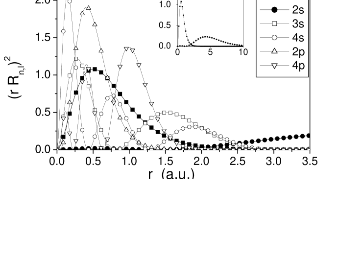
Figure 1: Our full CI (up to $4f$) $He$ $1s2s$ ${}^{1}S$ orbitals. The inset displays the ‘main’ orbitals, both contracted (lines), $E_{10}^{c}=-2.1459628$, $z_{1s}=1.992$, $b_{1s}=0.001$, $q_{1s}=3.195$, $z_{2s}=1.109$, $b_{2s}=0.373$, $q_{2s}=1.683$, and uncontracted (symbols), $E_{10}^{u}=-2.1459604$, $z_{1s}=1.992$, $z_{2s}=1.122$. We used the same virtual orbitals for both cases; the most significantly contributing have $z_{3s}=4.372$, $z_{4s}=8.257$, $z_{2p}=9.775$, $z_{4p}=24.483$. All quantities are in $a.u.$.