Metachronal wave and hydrodynamic interaction for deterministic switching rowers

Abstract

We employ a model system, called rowers, as a generic physical framework to define the problem of the coordinated motion of cilia (the metachronal wave) as a far from equilibrium process. Rowers are active (two-state) oscillators interacting solely through forces of hydrodynamic origin. In this work, we consider the case of fully deterministic dynamics, find analytical solutions of the equation of motion in the long wavelength (continuum) limit, and investigate numerically the short wavelength limit. We prove the existence of metachronal waves below a characteristic wavelength. Such waves are unstable and become stable only if the sign of the coupling is reversed. We also find that with normal hydrodynamic interaction the metachronal pattern has the form of stable trains of traveling wave packets sustained by the onset of anti-coordinated beating of consecutive rowers.

I Introduction

Cilia are hair-like extroflections of the cell membrane found in a variety of species from protists to humans, which contain active elements (molecular motors, filaments) acting as an internal drive book . Because of their size and typical velocities, the motion of cilia is in the low Reynolds number regime. Ciliary motion can be divided in two stages, called power and recovery strokes. The difference between the two is that in the power stroke a higher portion of the surface of the cilium pushes against the fluid compared to the recovery stroke so that, as in the breast stroke of human swimming, the two effective viscous drags are different, and the filament is able to propel the fluid Sleigh ; purcell ; BLA82 . Cilia normally appear in arrays, and show coordinated wave-like motion, referred to as metachronal wave. The behavior of the metachronal wave is thought to be strictly linked to the hydrodynamic interactions between cilia GLL97 ; gueron1 ; gheber ; gheber2 . The question of how these collective motions are generated, from the interplay between the internal, active degrees of freedom and the external interaction is still open. The scope of this work is to investigate this problem, using a simple deterministic model containing very few parameters, consistent with experimental observations and previous more detailed modeling, which can be easily simulated and solved analytically in the limit of large wavelengths.

Modeling of cilia GH55 ; Br72 ; HB78 normally requires including the infinite degrees of freedom of an inextensible line-like object, its bending elasticity, and its interaction with the fluid (slender body hydrodynamics), plus an active force, which can be imposed based on physical observations or treated starting from the “microscopic” internal active degrees of freedom Mu90 ; julicher . The model we present here (section II) is extremely simplified and economic in degrees of freedom. It is intended to be treatable analytically. The cilia are represented by point particles, two-state active oscillators which we call rowers. The active force is inspired by the switch mechanism introduced by Gueron and others gueron1 . Planar or linear arrays of interacting rowers are considered. In a previous work we used the same model to study the role of noise sto_row , proving that if the switch mechanism of single rowers is purely stochastic the hydrodynamic interaction generates metachronal waves which are statistically frustrated by the presence of random fluctuations, but can be stabilized by the presence of a short ranged coupling of the internal states, for example of chemical origin. An alternative scenario we proposed was that the presence of a coupling between position and transition frequency of the single rower would lead to wave like solutions. In this work we would like to pursue this second possibility, in the limiting case where the dynamics for the switch is governed deterministically by the configuration of the rower, as in the geometric switch of Gueron et alii.

After an introduction of the model (section II), we devote the main body of the paper (section III) to the onset of metachronal coordination. The discussion is divided in two parts. In the first we discuss an analytical solution of the continuum limit of our model equation, which enables to look for the onset of wave-like patterns with large wavelengths. In the second part we look at the short wavelengths through numerical simulations. As we will show, rowers with a deterministic configurational switch interacting hydrodynamically self-organize in patterns in which nearest neighbor particles beat in anti-phase, and propagate trains of wave packets with typical wavelength of a few particles. Only with an effectively attractive interaction do long-wavelength wave-like solutions appear.

II The model: rowers and evolution of the internal state

In the model we adopt, the movement of a single cilium is reduced to that of a low Reynolds number rower that maximizes the effective drag in its active phase (power stroke) and minimizes it in the passive, recovery stroke. More precisely, a rower is described by two degrees of freedom, of which the first, $f$ is translational and continuous and represents a displacement from a reference position. It can be thought of as the displacement of the center of mass of the filament from an equilibrium position. The second, $\sigma=\pm 1$, is discrete and labels the internal state of the object, active or passive. The rowing direction is fixed, while the orientation can in general be left open, to approach the problem of symmetry breaking in the generation of fluid flow sto_row . The two states carry different effective drags $\gamma_{\sigma}=1+\epsilon\sigma$ (with $\epsilon>0$) to the fluid, corresponding to different surface impacts of the rower (different shapes of the filament) in the two phases, together with different potentials (free energy landscapes) $V(f,\sigma)$, that generically describe different active or relaxation forces felt by the cilium. This is the implementation of the so-called scallop theorem purcell at this crude level of description, and makes it possible for a rower to generate a net flow in the fluid. There is no interaction between rowers other than the force propagated by the presence of the fluid. This force is modeled by the Oseen tensor for low Reynolds number flows, appropriate in the case of cilia purcell . The array of cilia is modeled as a linear or planar lattice of rowers labeled by the index $n$, and the configurations are specified by $f_{n},\sigma_{n}$.

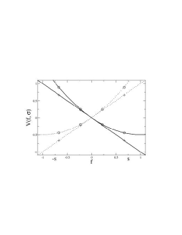
Figure 1: Potential $V(f,\sigma)$ for $k=0$ (+) and $k=1$ (o). The dotted lines indicate $\sigma=-1$, the solid lines $\sigma=1$.

This approach to the system contains a radical simplification in the degrees of freedom of the object, a string with infinite degrees of freedom, and of the active drive, generated by the collective behavior of many molecular motors. This reduction enables us to carry an analytical study. At our level of description, the substitution of cilia with point particles does not change qualitatively the interaction induced by the fluid. However, it’s a more delicate issue to reduce the collective motion of molecular motors to a single dynamic variable. We choose to maintain this variable discrete, justified by the experimental observation that the motion of a cilium is divided into two distinct phases and by previous, more detailed modeling that suggested this picture gueron1

The evolution of a rower internal state can be modeled generically as a stochastic process sto_row , defined by the transition frequencies between states. Here we analyze a limiting case where the transition frequencies depend singularly on the configuration in a way that reduces the dynamics to a deterministic one. Essentially, a rower contains a switch that alters instantaneously its internal state when a particular limit configuration is reached. The dynamics of the internal switch is entirely local, in the sense that there is no interaction of chemical origin between nearby rowers. With these choices, the evolution of $\sigma_{n}$ may be represented by the following equation containing a Dirac $\delta$ distribution

$$\frac{\partial\sigma_{n}(t)}{\partial t}=-2{\rm sgn}(f_{n}(t))\left|\frac{df_{n}}{dt}\right|\delta(f_{n}(t)-\textrm{s}\sigma_{n}(t))$$ (1)

where $\pm$s are the switch points in correspondence of which the discrete internal state is inverted. These parameters set the amplitude of oscillation of a single particle and determine its window of motion relatively to the driving potentials of the two states (figure 1).

Let’s now turn to the evolution of the rower displacement and the hydrodynamics. Considering the fact that an overdamped motion follows the maximum slope toward the minimum free energy and that we consider no metastability, there are generically two possible qualitative choices for the local conformation of the potentials in the two internal states. These can be linear, provided the system is far from a minimum, or quadratic if it is close. Therefore, rescaling all the constants that are not essential to our discussion (Stokes coefficient, prefactors), we write:

$$V(f,\sigma)=\frac{1}{2k_{\sigma}}(k_{\sigma}f-\sigma)^{2}-\frac{1}{2k_{\sigma}}$$

where the parameter $k_{\sigma}\in[0,1]$ determines the shape of the potential (figure 1). For consistency reasons, here s$<1$.

Thermodynamically,

• if the switch is close to a minimum of the energy, $k_{\sigma}=1$ and we take a quadratic potential, the rower has time to dissipate completely its excess energy to the environment before it reaches the switch. The dynamics is a cyclical repetition of such relaxation processes

• if the switch is far from a minimum energy configuration, $k_{\sigma}\to 0$ and the potential is linear. The switching process is faster than the thermalization time of the rower, that does not have time to dissipate all its energy. In this case at the switch the rower must undergo a collision-like process, which conserves the dissipation rate and the magnitude of the macroscopic velocity.

The considerations above refer generically to the active mechanism of model rowers, but leave aside the link with real cilia. If one wants to give this drive a microscopic interpretation, it has to be in terms of collective motions of the internal motors and elastic degrees of freedom of the cilium. For example, in the linear potential scenario one can imagine that motors attach/detach slowly generating a constant force, while in the nonlinear one they attach simultaneously, giving the cilium a well-defined minimum energy curvature, and they detach collectively after reaching it. In what follows we will set $k_{\sigma}=k$ for simplicity.

The equation of motion for the rowers has to contain the hydrodynamic interaction. We think of rowers as sources for the velocity field and not as boundary conditions, which means introducing a (nondimensional) coupling constant $\alpha$ between the fluid and the rowers as a substitute for the geometric constraints. $\alpha$ is proportional to the Reynolds number, or to the inverse of the kinematic viscosity. To avoid complications, we do not take into account additional boundary conditions, such as walls, but it is straightforward to include them in the model. As the system is in a low Reynolds and Strouhal number regime landau , it is possible to use the regularized Oseen tensor Doi to eliminate the velocity field and obtain an evolution equation for the sole rowers degrees of freedom sto_row :

$$\frac{df_{n}(t)}{dt} = (1+\epsilon\sigma_{n}(t))\frac{\partial[-V(f_{n}(t),\sigma_{n}(t))]}{\partial f_{n}}+$$ (2)

$$+ \alpha\sum_{m\neq n}\Omega[{n},{m}]\frac{\partial[-V(f_{m}(t),\sigma_{m}(t))]}{\partial f_{m}}$$

where $\epsilon$ is the parameter that represents the difference between the effective viscous drags in the two states and $\Omega[{n},{m}]=\frac{1}{r_{nm}}\hat{\mathbf{x}}\hat{\mathbf{x}}(I+\mathbf{\hat{r}}_{nm}\mathbf{\hat{r}}_{nm})$ is the Oseen tensor projected on the beating direction $\hat{\mathbf{x}}$ of the rowers. Strictly speaking, $\Omega[{n},{m}]$ depends on $f_{n},f_{m}$. However, to ease things in an analytical calculation, we approximated it with a quantity that depends only on the relative distance of the lattice sites, assuming that the oscillations are small compared to this distance. Most of our simulations, though, were carried with the full $\Omega$.

III Metachronal coordination

The scope of this section is to establish whether hydrodynamic interactions are sufficient to re-phase the rowers in absence of a more direct coupling of chemical or mechanical origin. The oscillatory motion of a single rower in an array is guaranteed by the structure of its equation of motion. A mean field description of the array can be carried out considering the overall effect of the velocity field generated on one rower by all the others. This procedure is outlined in appendix A, and leads to the main result that a collection of rowers can generate a macroscopic flow if $\epsilon\neq 0$, and that, provided there is no intrinsic orientation in the beating mechanism, symmetry will be broken. However, in a description that goes beyond mean field, nothing can be said about the beating time, which can in general vary with the dynamics, so that the question can be restated as whether this variability in the beating time is stabilized or disrupted by the hydrodynamic interactions. The problem is hard to approach analytically due to the discontinuous nature of the switch $\sigma$ and the nonlinearities. However, the continuous limit of the model, which describes the long wavelength behavior of the system, can be approached analytically. The results obtained in this way can then be compared with the numerical study of the discrete case.

From the point of view of solving the equation of motion one has to investigate:

• The existence of wave-like solutions. We define metachronal waves motions of the kind $f_{n}(t)=f(t\pm\tau\mathbf{x_{n}})$, and simple metachronal waves those for which $f$ (and thus $\sigma$) is a periodic function.

• The stability and attractivity properties of these solutions.

• Their statistical weight in a macroscopic description of the system on large time scales. As one cannot establish a priori its initial conditions, the metachronal solutions will be significant if the phase space volume of the initial conditions they attract is nonzero, and the relaxation time scales do not exceed a cutoff defined by the lifetime of the system.

In what follows we will be mainly concerned with the first two points. The third point will be approached in general numerically for systems of a few rowers (short wavelengths).

III.1 Metachronal pattern in the large wavelength limit. Continuous model

We will show that in the continuum limit of the equation of motion 2 it is possible to find simple metachronal wave solutions and study their stability analytically. We can take the continuous limit analyzing selectively metachronal solutions whose wavelength is large compared to the spacing between rowers. Then $f_{n}(t)=f(\mathbf{x_{n}},t)$ becomes the continuous field $f(\mathbf{x},t)$ and we can rewrite the hydrodynamic interaction tensor $\Omega[n,m]$ as $(-\nabla^{2}+q^{2})^{-1}$, where we incorporate also the possibility of screening with inverse screening length $q$. With one inversion of this operator, the evolution equation 2 for the continuous $f$ can be written as

$$(q^{2}-\nabla^{2})\left[\frac{\partial f}{\partial t}+(1+\epsilon\sigma)(kf-\sigma)\right]=-\alpha(kf-\sigma)$$ (3)

The laplacian in the above expression is one dimensional, along the fixed direction of beating $\hat{\mathbf{x}}$ . We look for planar metachronal wave solutions with the ansatz $f=f(t-\tau x)$, so that we can reduce to a 1+1 dimensional problem. The transverse hydrodynamic interactions are irrelevant as the rowers are constrained to beat in one dimension, and the anisotropic terms can be absorbed in the prefactor of the interaction tensor. Calling $y=t-\tau x$, we can assume without loss of generality that $y=0$ is the coordinate of a wave-front, where the switch $\sigma$ has a jump. This translates in the condition

$$\sigma=\theta(-y)-\theta(y)$$

where $\theta$ is the Heaviside step function. The local displacement $f$ can be decomposed in the sum of power stroke and recovery stroke parts, $f_{+}\theta(-y)+f_{-}\theta(y)$, this implies that

$$\sigma f=f_{+}\theta(-y)-f_{-}\theta(y)$$

With this procedure one obtains two linear third order differential equations for $f_{-}$ and $f_{+}$, together with four joining conditions for $f_{\pm}$ and their derivatives in correspondence with the jumps of $\sigma$. Metachronal solutions can be constructed starting from the initial condition $y^{(0)}=0$ and generating a succession of wave-front coordinates $y^{(1)},y^{(2)}\ldots y^{(n)}$ imposing the joining conditions above on the solutions of the third order differential equations for $f_{\pm}$. The iteration of this process, starting from the initial conditions for $f_{\pm}$ and its first and second derivatives, or equivalently on the vector of the (two at the most) independent arbitrary constants $(A_{\pm},B_{\pm})$ of the solution of the differential equations, generates a flux in phase space, described by an affine transformation. The existence of a fixed point of the succession $(A^{(n)}_{\pm},B^{(n)}_{\pm})$ and its attractive properties determine the nature and stability of the constructed metachronal wave. At every iteration, the $y^{(n)}$ must satisfy the relation $f(y^{(n)})=\pm\textrm{s}$. Note that despite every step involves linear operations, a strong nonlinearity is introduced by the inversion for $y^{(n)}$ of the solutions of the differential equations. It is also important to stress that the solutions constructed in this way are in general not periodic, and may have a domain of existence which is bounded in $y$, as after a number of iterations it could be impossible to invert for $y^{(n)}$. More details on these calculations for the exemplifying case $k=1,\epsilon=0$ are reported in appendix B.

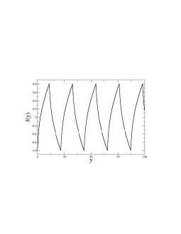
Figure 2: Analytical solution of the continuum equation (3) computed for the case s $=0.8$, $p=0.01$, $k=1$. The fixed point values of the parameters in this case are $A_{\pm}=-0.435,B_{\pm}=-1.456$.

Our results can be summarized as follows. We find that, from the point of view of the existence and stability of metachronal solutions, $\epsilon$ plays no qualitative role, so that the problems of flow-generation and syncronization can be separated. For this reason, the discussion is independent on $\epsilon$ and can be simplified restricting to the case $\epsilon=0$. A necessary condition to find $y^{(n)}$ is that s $<1$, which gives a good consistency test.

• For quadratic potentials ($k>0$) the qualitatively relevant parameter is $p=\frac{q+\alpha}{\tau^{2}}$. Fixing s, there is a critical value $p_{c}$ such that for $p>p_{c}$ there exist no solution. This set an upper critical wavelength $\lambda_{c}$ for the metachronal waves. For $0<p<p_{c}$, a fixed point exists, and the stability analysis gives a marginally stable saddle point in the planes of coefficients ($A_{\pm},B_{\pm}$). In other words there is one line (a region of zero measure) of stability in this plane, with runaway hyperbolic trajectories around it. We report this case in figure 3 as an example. Finally, for $p<0$ the wave like solutions are always stable. However, this last condition implies $p<0$, therefore an effective “attractivity” of the hydrodynamic interactions. We will discuss below two cases that could lead to this situation.

• In the case $k=0$ (linear potentials) the solution always exists. Stability analysis gives solutions that are always unstable (two eigenvalues $>1$) for $p>0$ and stable for $p<0$.

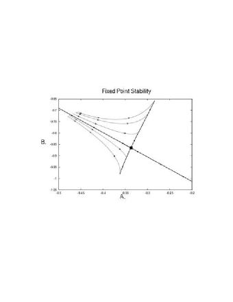
Figure 3: Stability analysis for s$=0.3$, $p=0.05$, $k=1$. The fixed point values of the parameters are $A_{\pm}=\pm 0.337,B_{\pm}=\pm 0.865$. The fixed point is marked with a black square, and the lines with arrows indicate the direction of evolution of different initial conditions, showing that the fixed point is marginally stable. The trajectories are obtained iterating the transformation on $(A_{\pm},B_{\pm})$ starting from different initial conditions. The lines reported are Bezier interpolations of these (discrete) transformations.

In both cases we can conclude that metachronal solutions at long wavelengths are unstable unless $p<0$, and the interaction becomes attractive. We would like to spend a few words on the possible physical meaning of this change in sign, with an effectively attractive interaction. One first consideration is that interaction between colloidal objects can be more complicated than how we represent it, in presence of hydrodynamic effects or charge. For example, it has been speculated that the presence of a wall in combination with a surface charge, all neglected in our model, lead to effectively attractive potentials between colloids of like charges brenner . Lubrication forces are another possibility, provided that cilia are able to get sufficiently close to each other. For rowers, this last condition is contrary to the assumption of small oscillations in the theoretical calculation but can be tested through simulations with the full Oseen tensor. Coming back to the more orthodox case $p>0$, the results above show that in the continuous limit simple metachronal waves (with nearest neighbor rowers in phase) exist for all wavelengths (below a characteristic one, for $k\neq 0$), but they are (marginally for $k\neq 0$) unstable. These results are not sufficient to establish in general the statistical behavior of metachronal waves, as the hypotheses adopted here reduce the analysis to a particular class of solutions and the local region of the phase space that surrounds them. For negative $p$ only we can conclude that wave-like solutions attract all the initial conditions. In the other cases, where the solutions are not attractive, we have to look for other basins of attractions in the phase space. One possibility is that these lie in the shorter wavelength region, which is overlooked by the continuous model. This motivates the numerical analysis of the next sections.

III.2 Numerical simulations with many rowers

A confirmation of these results, and more insight on the behavior of the system comes from numerical simulations of linear and two dimensional arrays of many (50-250) rowers. These were run starting from random initial conditions, with nearest neighbor Oseen-like interactions, the simplified interaction tensor $\Omega[n,m]$ and the full $\Omega[f_{n},f_{m}]$, robustly showing the same phenomenology in all cases. In particular, for linear arrays with $k>0$:

• For $p>0$ the relaxed solutions look like trains of traveling wave packets where nearby rowers show anti-coordinated motion. In the patterns observed in the simulations the packets have typically a characteristic length of the order of 10 particles. Their traveling direction coincides almost always with the beating direction of single rowers.

• For $p<0$ long wavelength traveling solutions appear. These always have a wavelength that is exactly the size of the array. For every solution of this kind traveling in one direction, there is another one in the opposite one, leading to mirror symmetric standing waves. The same solutions are found if $\alpha$ is kept positive, and a nearest neighbor attractive interaction is added.

This is exemplified in figure 4. For linear arrays with $k=0$ wave-like solutions appear only for $p<0$. Two dimensional arrays show the same qualitative behavior. This makes the wave patterns propagate in directions that are different from the beating direction of the rowers (non-simplectic, in the language of metachronal waves).

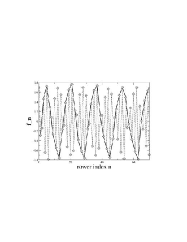
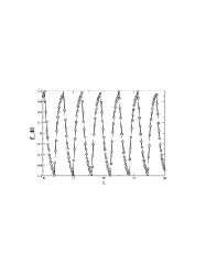
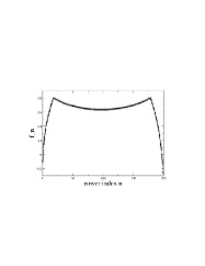
Figure 4: Metachronal solutions from numerical simulations of linear arrays of rowers interacting with the full Oseen tensor. The distance between successive rowers is 2 in our rescaled units and $\epsilon=0.25$. (a) and (b): case $p>0$. $\alpha=0.4,k=1,150$ rowers. In (a) a part the configuration $f_{n}$ as a function of the rower index is shown. The dashed line shows the actual configuration, while the solid one, obtained connecting the points relative to odd rowers, outlines the shape of the wave packet. (b) represents the time evolution $f(t)$ of the 40th rower of this array. (c): case $p<0$. $\alpha=-0.1,k=1,200$ rowers. The configuration $f_{n}$ shows a long wavelength metachronal wave. The part of the configuration for $i>100$ is mirror symmetric, due to the same pattern traveling in the opposite direction

We can give a heuristic argument based on the switch mechanism to account for this anti-phase coordination. Let’s consider three consecutive rowers X,Y,Z, and suppose they are in phase. Immediately after X reaches the +1 switch it feels a strong negative force due to the change in the potential, which is propagated mainly to Y and much less to Z. Provided Y was going toward the same switch, it will be slowed down, and therefore de-phased with respect to X. If we imagine now that X,Y,Z are in anti-phase and A reaches the +1 switch. Now the force felt by Y (and much less by Z) will be driving it toward the -1 switch, reinforcing the dephasing. As a result, the anti-phase beating between X and Y is more stable than the coordinated motion. According to this argument, this will be the case in all the instances where the influence of nearest neighbors is stronger than that of far away ones. More formally, one can find a reason for this behavior in the analytical solution of the continuum equation. Configurations where rowers, interacting with the normal Oseen tensor have opposite phase are overlooked by the continuum limit. However, roughly speaking, these configurations lead effectively to a change of sign of $\alpha$ in the continuum limit equation, as one can easily see imposing $f_{\textrm{\tiny even}}=-f_{\textrm{ \tiny odd}}$ in equation 2. Therefore one can think that the stable waves found for $p<0$ in the continuum model have a trace of this anti-phase behavior.

III.3 Stability of the metachronal wave at short wavelengths.

To analyze the system at shorter wavelengths we ran numerical simulations of linear arrays of a few rowers with periodic boundary conditions, choosing to truncate the interaction to nearest neighbors. We interpret the boundary condition as a constraint on the wavelength of the resulting wave patterns. For up to four rowers, we analyzed the system using Poincaré maps. This study leads to more general considerations on the statistical weight of metachronal solutions. The maps are obtained graphing the positions of two rowers when a reference one reaches the switch over many cycles of the motion and for different initial conditions. If the resulting graph is, or converges to a single point, the motion is coordinated. If it is a closed orbit the coordination is quasi-periodic, which means that the motion in general does not look like a traveling wave. Finally, if the resulting graph is a random scatter plot, the motion is chaotic. Indeed, the system can be either chaotic or quasi-periodic if the potentials are linear, ($k=0$), as can be seen in figure 5. The phase space volume of the quasi-periodic region delimited by the concentric loops is therefore a measure of the statistical weight of quasi-periodic solutions. The volume of this region decreases with increasing $\alpha$.

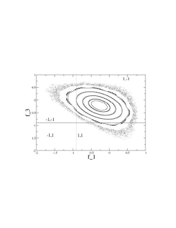
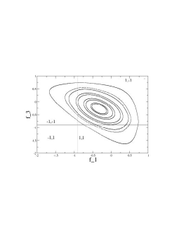
Figure 5: Poincaré map for the case $k=0$, three rowers, periodic boundary conditions. Here, $\epsilon=0.02$ and s$=0.9$. The allowed configurations are confined in the square region [-s,s]$\times$[-s,s]. However, to increase clarity, the figures were divided in four regions, corresponding to the different values of the two switches, which were “folded outside”, so that the axes correspond to the actual configuration of the rowers after a mirror reflection dependent on the state of the switches. (a) $\alpha=0.1$. (b) $\alpha=0.01$.

The case $k\neq 0$ is somewhat different. Here, there is no chaos, and the stable tori become attractors to a fixed point of the parameter space (figure 6, (a)). This means in principle that all the initial conditions lead to pattern formation. Therefore, the relevant parameter becomes the relaxation time. This diverges as $k\rightarrow 0$ as a power-law with exponent $b\simeq 0.85$ and as $\alpha\rightarrow 0$ with exponent $c\simeq 0.74$.

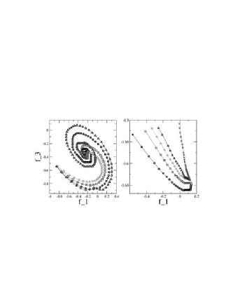
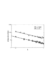
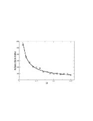
Figure 6: (a) Poincaré maps for $k\neq 0$, three rowers, $\epsilon=0.02$. Left: $\alpha=0.01$ attracting trajectories for different values of $k$. $\triangle$ $k=0.15$. O $k=0.2$. $\Box$ $k=0.3$. $\Diamond$ $k=0.4$. Right: different initial conditions for $k=1$. (b) log-log plot of the relaxation time as a function of $k$ for $\alpha=0.01(\Box)$ and $\alpha=0.1$ (O). The power law fits (solid lines) yield an exponent of $0.85$. (c) Relaxation time as a function of $\alpha$ for $k=0.3$. The power law fit gives the exponent $0.74$.

The curvature of the potential, which as we discussed has to do with the activity of the microscopic active degrees of freedom, seems therefore to be important in determining the organization properties of the system. On the other hand, the phenomenology observed for different values of $\alpha$ is qualitatively consistent with what observed experimentally for arrays of cilia beating in fluids with varying viscosity gheber2 ; gheber .

IV Overview and conclusions

We have presented a simple model system of two-state low Reynolds number oscillators called rowers as a generic framework for the problem of cooperation of cilia. The dynamics adopted in this work, specified setting the transition rates between the two potentials, is entirely deterministic, determined by a switch mechanism coupled to the configuration. We solved analytically for wave like solutions the continuum, long wavelength, limit of the equation of motion for an array of rowers with hydrodynamic interaction and we analyzed the stability of the solutions, confronting with results from numerical simulations. Finally, we analyzed through Poincaré maps the phase space dynamics of systems of a few rowers, to study their behavior at short wavelengths.

Our most important result is that metachronal patterns exist at all wavelengths (below a characteristic one, for $k\neq 0$), but long wavelength solutions are (marginally for $k\neq 0$) unstable. The stable patterns have the form of consecutive wave-packets where nearest neighbor oscillators are in anti-phase, propagated with constant speed, with a characteristic length of a few rowers. We showed that the statistical weight of these solutions can be determined numerically imposing an upper cutoff on the wavelength of the pattern. Only in the presence of a reversed coupling constant, can long wavelength metachronal solutions be stable. We proposed two possible physical reasons for this reversal in sign. Deterministic switching rowers, as two state oscillators, show a rich and unusual phenomenology, of which we could explore a number of aspects. Their behavior is in many ways opposite to our usual notion of oscillations, starting from the fact that no normal modes can be defined, but the oscillators self-tune to a chosen frequency determined by the characteristic relaxation times in the two states, much as in systems close to a Hopf bifurcation julicher .

Comparing the behavior our abstract entities with that of real or model cilia, the first puzzling question seems to lie in the anti-phase motion. As discussed, a solution of this could lie in a short ranged interaction with a different origin. One good candidate for this are lubrication forces, as real cilia can be really close to each other. Also, a short ranged synchronization between the switches of chemical origin could lead to the same result, consistently with the scenario proposed in our previous work. The relevant parameters in our discussion are the stiffness of the potential $k$ and the hydrodynamic interaction coupling strength $\alpha$. The first is related to the internal active degrees of freedom, which are hard to access experimentally, while the second can be used for a qualitative comparison of our results with experiments where arrays of cilia are observed beating in fluids with varying viscosity gheber2 ; gheber . One other question is the relation with more detailed models of cilia and their internal drive, in particular with the geometric switch model of Gueron and collaborators GLL97 ; gueron1 . Rowers, with their few degrees of freedom constitute a system much more under control than filaments to test. We can conclude that generically simple hydrodynamic interaction does not synchronize but anti-synchronizes nearest neighbor rowers, so that, if filamentous objects are to be synchronized by a similar mechanism, an extra (to be found) ingredient is needed.

Appendix A Mean field approach, symmetry breaking

It is possible to estimate the magnitude of the characteristic beating times and the macroscopic speed generated on the fluid without having to solve explicitly the equations of motion, using simple self-consistency considerations sto_row . This is done writing the equations of motion (1 and 2) for a single rower in a constant external effective velocity field $\mathbf{v}$ along its beating direction and supposing that this velocity is generated by the effect of the surrounding rowers. Equation 2 looks then like

$$\frac{df_{0}(t)}{dt}=(1+\epsilon\sigma_{0}(t))\frac{\partial[-V(f_{0}(t),\sigma_{0}(t))]}{\partial f_{0}}+v$$

where we labeled conventionally with the index 0 the rower around which we do the selfconsistent calculation. It is then straightforward to calculate the beating times $t_{\pm}$ for this single rower, defined as the times required to go from -s to +s and back respectively:

$$\begin{array}[]{c}t_{+}=[k(1+\epsilon)]^{-1}ln\left[\frac{(1+\epsilon)(1+k\,\textrm{s})+v}{(1+\epsilon)(1-k\,\textrm{s})+v}\right]\\ \\ t_{-}=[k(1-\epsilon)]^{-1}ln\left[\frac{(1-\epsilon)(1-k\,\textrm{s})-v}{(1-\epsilon)(1+k\,\textrm{s})-v}\right]\end{array}$$

These quantities can be used to determine self-consistently the absolute value of the “macroscopic” fluid velocity $v$, taking into account the average force exerted by the single rower on the fluid in one cycle.

$$v_{\textrm{sc}}=\left[\alpha\sum_{n\neq 0}\Omega_{0,n}\right]\frac{1}{T}\int_{0}^{T}-\frac{\partial V(f,\sigma)}{\partial f}dt$$

where the total period $T=t_{+}+t_{-}$ depends on $v$. Therefore

$$v_{\textrm{sc}}=-\frac{1}{T}\left[\alpha\sum_{n\neq 0}\Omega_{0,n}\right]\left[v_{\textrm{sc}}\left(\frac{t_{+}}{1+\epsilon}+\frac{t_{-}}{1-\epsilon}\right)+4\epsilon\,\textrm{s}\right]$$ (4)

In this expression the summed hydrodynamic propagator simply plays the role of a multiplicative constant, and s determines the self-consistent value for the velocity (see figure 7). For $\epsilon=0$, $v_{\textrm{sc}}=0$, and the scallop theorem is found again in the description of a collection of rowers.

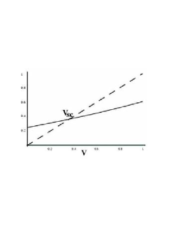
Figure 7: Selfconsistent velocity calculation. The right hand side (solid line) and the left hand side (dashed line) of equation 4 are plotted as a function of $v$ in the graph above. The intersection between the two lines yields $v_{\textrm{sc}}$. The values of the parameters for the curves shown are $k=0.8,\epsilon=0.25,\textrm{s}=0.8$, and $\alpha\sum_{n\neq 0}\Omega_{0,n}=0.2$. With these values, $v_{\textrm{sc}}\simeq 0.365$ in nondimensional units.

The same argument yielding a non zero self-consistent velocity can be extended to the case of one - or a collection of- rowers whose rowing direction is not fixed. This is obtained taking reflection symmetric potentials $V(f,\sigma)=V(-f,\sigma)$, one of which with a single minimum for $f=0$, the other with a double well. A thermal noise needs to be added for the problem to be well posed. Rowers are able to break spontaneously the symmetry to generate a flow in the fluid sto_row . For real cilia, the problem of symmetry breaking can be relevant in the context of generation of left-right asymmetry through nodal flow in vertebrate embryos nonaka .

Appendix B Example of explicit solution of the continuous model and its stability

We will solve equation 3 analytically with the ansatz $f=f(x-\tau t)$ on the solution. For simplicity we can restrict ourselves to the case $k=1$, $q=0$, $\epsilon=0$, as the general case carries no further conceptual complication. Calling $y=x-\tau t$, the equation reads:

$$-\tau^{2}(f^{{}^{\prime\prime\prime}}+f^{{}^{\prime\prime}})+\alpha(f-\sigma)+\tau^{2}\sigma^{{}^{\prime\prime}}=0$$ (5)

where ^′ indicates derivatives with respect to $y$. For a transition of $\sigma$ from 1 to -1 at the wave-front $y=0$, the right joining conditions are, as already discussed,

$$\sigma=\theta(-y)-\theta(y)$$ (6)

$$f=f_{+}\theta(-y)+f_{-}\theta(y)$$ (7)

$$\sigma f=f_{+}\theta(-y)-f_{-}\theta(y)$$ (8)

where $\theta$ is the Heaviside step function, and $f_{\pm}=f_{\pm}(y)$. Analogue expressions hold for the transition $-1\rightarrow 1$. The decompositions above generate two linear ordinary differential equations for $f_{\pm}$.

$$f_{\pm}^{{}^{\prime\prime\prime}}+f_{\pm}^{{}^{\prime\prime}}-pf_{\pm}=\mp p$$ (9)

with $p=\frac{\alpha}{\tau^{2}}$. Moreover, the same conditions 6, 7, 8 and their derivatives can be substituted in equation 5, obtaining an expression containing terms in $\theta(\pm y)$, $\delta(y)$ and its derivatives. Equating all the terms to zero one obtains three joining conditions. That is,

$$(f_{+}-f_{-})|_{\textrm{switch}}=0;$$ (10)

$$(f^{{}^{\prime}}_{+}-f^{{}^{\prime}}_{-})|_{\textrm{switch}}=\frac{2}{3};$$ (11)

$$(f^{{}^{\prime\prime}}_{+}-f^{{}^{\prime\prime}}_{-})|_{\textrm{switch}}=-\frac{4}{9}$$ (12)

Here, and more generally in the case $\epsilon=0$, the two equations 9 are the same with the identification $-f_{-}=f_{+}$. The solution of equation 9 is easily obtained; $f_{\pm}=\pm 1$ is always a particular solution, and one has to solve the characteristic equation $z^{3}+z^{2}=p$. This admits three real solutions for $0<p<\bar{p}$, and one for $p<0.p>\bar{p}$, $\bar{p}=4/27$. We will analyze in detail here the case with three solutions ($-z_{1},-z_{2},z_{3}$), with $z_{1},z_{2},z_{3}>0$ . In this situation,

$$f_{\pm}(y)=\pm\left(1+A_{\pm}e^{-z_{1}y}+B_{\pm}e^{-z_{2}y}+C_{\pm}e^{z_{3}y}\right)$$

The constant $C_{\pm}$ can be eliminated using the condition $f_{\pm}(0)=\mp\textrm{s}$, meaning that after the first jump the rower is located at the switch. The next step is to evolve this solution up to a certain $y_{\pm}$ where the next switching event will take place, imposing that

$$f_{\pm}(y_{\pm})=\pm\textrm{s}$$ (13)

$y_{\pm}$ is obtained inverting this last expression, and has to satisfy the joining conditions 12 for the next “piece”. For example, supposing we start from state $\sigma=1$

$$(f^{{}^{\prime}}_{+}(y_{+})-f^{{}^{\prime}}_{-}(0))=\frac{2}{3}\ ;\ \ (f^{{}^{\prime\prime}}_{+}(y_{+})-f^{{}^{\prime\prime}}_{-}(0))=-\frac{4}{9}$$

This gives a linear transformation $(A_{+},B_{+})\rightarrow(A_{-},B_{-})$. A complete solution can be constructed iterating this procedure. This solution is in general non-periodic, as $y_{\pm}$ may vary at every step, and also cease to exist. The equations that determine $y_{+}^{(n)}$ and $y_{-}^{(n)}$ at the $n$-th step can be written as

$$A_{\pm}^{(n)}H_{(1,3)}(y_{\pm}^{(n)})+B_{\pm}^{(n)}H_{(2,3)}(y_{\pm}^{(n)})-(1+\textrm{s})E_{3}(y_{\pm}^{{(n)}})+(1-\textrm{s})=0$$ (14)

where we used the notation

$$H_{(i,3)}(y)=e^{-z_{i}y}-e^{-z_{3}y}\quad i=1,2$$

$$E_{i}(y)=e^{-z_{i}y}\quad i=1,2;\quad E_{3}(y)=e^{-z_{3}y}$$

The joining conditions for step n are

$$\begin{array}[]{c}A_{\pm}^{(n+1)}=E_{1}(y_{\mp}^{(n)})A_{\mp}^{(n)}+w_{1}\\ B_{\pm}^{(n+1)}=E_{2}(y_{\mp}^{(n)})B_{\mp}^{(n)}+w_{2}\end{array}$$ (15)

where $w_{1},w_{2}$ are rational functions of the solutions $z_{1},z_{2}z_{3}$.

A simple (periodic) metachronal solution exists when the transformation has a fixed point, which can be imposed setting the equality between $A_{+}^{(n+1)}$ and $A_{+}^{(n)}$. This wave is characterized by a unique $y_{+}=y_{-}=\bar{y}$ solution of

$$\frac{w_{1}}{1+E_{1}(\bar{y})}H_{(1,3)}(\bar{y})+\frac{w_{2}}{1+E_{2}(\bar{y})}H_{(2,3)}(\bar{y})-(1+\textrm{s})E_{3}(\bar{y})+(1-\textrm{s})=0$$

and by coefficients $A_{-}=A_{+}\equiv\bar{A},\quad B_{-}=B_{+}\equiv\bar{B}$ given by

$$\bar{A}=\quad\frac{w_{1}}{1+e^{-z_{1}\bar{y}}}$$

$$\bar{B}=\quad\frac{w_{2}}{1+e^{-z_{2}\bar{y}}}$$

The equation for $\bar{y}$ admits solution only if s $<1$, and, for any given value of s, if $p$ is lower than the critical value $p_{c}<\bar{p}$ introduced in the paper, which can be found numerically. This sets a maximal wavelength $\lambda_{c}$ for the metachronal wave. The stability of the solution can be evaluated linearizing the flow, starting from the point $(\bar{A}+\delta A,\bar{B}+\delta B)$ in parameter space, inverting equation 14 for $\bar{y}$ and calculating the total variation $(\delta A,\delta B)$ from 15. In this case this yields one negative and one positive eigenvalue corresponding to a marginally stable fixed point. The procedure outlined in this appendix can be carried out more in general, leading to the results discussed in the body of the paper.

References

- (1) D.Alberts, et. al. The Molecular Biology of the Cell, (Garland, NY, 2002).
- (2) Cilia and Flagella, edited by M.A.Sleigh, (Academic Press, London, 1974).
- (3) E.M.Purcell, Am. Jour. of Phys.,45, 1 (1977).
- (4) J.R.Blake, N. Liron, and G.K.Aldis, J.Theor.Biol. 98, 127 (1982).
- (5) S.Gueron, K.Levit-Gurevitch, N. Liron, Proc. Nat. Acad. Sci. USA 94, 6001 (1997).
- (6) S.Gueron, K.Levit-Gurevich Proc. Nat. Acad. Sci. USA 96, 22:12240 (1999).
- (7) L.Gheber, Z.Priel Cell Motil. Cytoskeleton 16, 167 (1990).
- (8) L.Gheber, A.Korngreen, Z.Priel, Cell Motil. Cytoskeleton 39, 9 (1998).
- (9) J.Gray, and G.Hancock ,J.Exp.Biol. 32, 802 (1955).
- (10) C.J.Brokaw, Biophys. J. 12, 564 (1972).
- (11) M.Hines, J.J.Blum, Biophys. J. 23, 41 (1978).
- (12) M.Murase, J.theor.Biol. 146, 209 (1990).
- (13) S.Camalet and F.Julicher, New J. Phys. 2, p.24 (2000).
- (14) M.Cosentino Lagomarsino, B. Bassetti, P. Jona, Eur. Phys. J. B 26, 81 (2002).
- (15) L.D.Landau, E.M.Lifshitz Fluid Mechanics (Butterworth-Heinemann, Oxford 1998).
- (16) M.Doi, S.F.Edwards The Theory of Polymer Dynamics (Oxford Univ. Press, London, 1986).
- (17) S.Nonaka, et. al. Nature 418, 96 (2002).
- (18) D.Rossi, Thesis. Università degli studi di Milano (2002).
- (19) T.M.Squires, M.P. Brenner, Phys. Rev. Lett. 85, 4976 (2000).