Finite-Time Singularity Signature of Hyperinflation

Abstract

We present a novel analysis extending the recent work of Mizuno et al. [7] on the hyperinflations of Germany (1920/1/1-1923/11/1), Hungary (1945/4/30-1946/7/15), Brazil (1969-1994), Israel (1969-1985), Nicaragua (1969-1991), Peru (1969-1990) and Bolivia (1969-1985). On the basis of a generalization of Cagan’s model of inflation based on the mechanism of “inflationary expectation” or positive feedbacks between realized growth rate and people’s expected growth rate, we find that hyperinflations can be characterized by a power law singularity culminating at a critical time $t_{c}$. Mizuno et al. [7] ’s double-exponential function can be seen as a discrete time-step approximation of our more general nonlinear ODE formulation of the price dynamics which exhibits a finite-time singular behavior. This extension of Cagan’s model, which makes natural the appearance of a critical time $t_{c}$, has the advantage of providing a well-defined end of the clearly unsustainable hyperinflation regime. We find an excellent and reliable agreement between theory and data for Germany, Hungary, Peru and Bolivia. For Brazil, Israel and Nicaragua, the super-exponential growth seems to be already contaminated significantly by the existence of a cross-over to a stationary regime.

, ,

1 Introduction

Inflation is the economic situation in which prices apparently move monotonically upward and the value of money decreases. To classical economics, inflation is the undue increase in the supply of credit above the level that is supported by current savings. High inflation is always associated with high rates of money supply growth while the relationship is weak for countries with low inflation [2]. Thus, fighting high inflation requires reducing the growth rate of the money supply.

Inflation is one of the few big issues in macroeconomics, together with unemployment, monetary policy, fiscal policy, import-export deficits, productivity, government spending and the business cycle, and has been at the forefront of public battles over the past half-century. A good economic policy should strive to achieve a balance between often contradictory requirements: for instance, many economists assume that unemployment tends toward a natural rate below which it cannot go without creating inflation. Samuelson and Solow had brought to the U.S. the empirical evidence, first compiled by the British economist A.W. Phillips, that there seems to be a tradeoff between inflation and unemployment–that is, higher inflation meant lower unemployment. There is thus a long tradition among economists to adopt monetary policy as a way to keep the economy running on high-employment overdrive. Allowing prices to rise seemed the only humane thing to do. Friedman argued however that the unemployment/inflation tradeoff was temporary, and he also pointed out that using fiscal and monetary policy to avert recessions was a lot harder than it looked. The difficulties stem from the fact that policies designed to restrain inflation by lowering the level of aggregate demand will tend to depress investment and harm capacity. Improved industrial performance requires a climate conducive to investment and research and development, which in turn depends on, inter alia, high and stable levels of aggregate demand. Business and inflation cycles often result from the combination of endogenous interactions (that can lead to incoherence) and of the effects of institutions to contain these tendencies in the economy. The corresponding economic times series can exhibit smooth growth and well-behaved cycles as possible transitory results of the economic processes, but can also allow for intermittent conditions conducive to the emergence of incoherence or turbulence. Institutional factors attempt to act as circuit breakers on the economy. Whenever institutionally determined values dominate endogenously determined values, the path of the economy is broken and an interactive process, which starts with new initial conditions, generates future values. Specifically, whenever the economy threatens to behave incoherently, these stabilizers, whether built-in or activated by government authority, prevent the economy from continuing on the prior determined path, with the corresponding added complication and possible elements of destabilization. These are important elements in the path evolution of inflation.

In standard economic theory, inflation is associated with money supply growth. At equilibrium, money determines price level and implies equilibrium in markets for other assets. At equilibrium, money demand depends primarily on income and interest rates. But there are several factors keeping money demand unstable, such as financial innovations as well expectations. Indeed, one of the major causes of the complexity in stabilizing inflation together with other macroeconomic variables is that expectations of producers, consumers and investors may play a key role in the dynamics. Indeed, investment allocations or inflation expectations are influenced by ex-ante values of the risk premia and ex-post returns are rough approximations of these. Thus, “inflationary expectation” occurs when people begin to raise prices not because of actual changes in supply or demand or cost or the size of the money supply, but out of fear that some such changes might happen. In the 1990s, when Alan Greenspan, the chairman of the US federal reserve, said that the U.S. was still suffering from the inflationary expectations caused by the monetary excess of the 1970s, he was directly addressing the potential for inflation caused by “inflationary expectations.” When European central banks added liquidity to the gold market in an attempt to prevent an increase in the price of gold from creating concerns about a decrease in the value of the dollar, they were addressing the psychological component of price stability involved in “inflationary expectations.” Mathematically, this dynamics translates into sets of coupled nonlinear equations expressing both the competition and delays between expectations and realizations and the presence of positive and negative feedback loops. The complexity of the resulting dynamics stems from the complex nonlinear negative and positive feedback processes intertwining the different component of policies.

There are several causes of inflation. A prominent origin is wars, which cause the type of inflation that results from a rapid expansion of money and credit. For instance, in World War I, the American people were characteristically unwilling to finance the total war effort out of increased taxes. This had been true in the Civil War and was also so in World War II and the Vietnam War. Much of the expenditures in World War I, were financed out of the inflationary increases in the money supply. If money supply growth and real income are constant, then expected inflation rate equals current inflation rate (assuming no change in elasticities). This is more or less the standard situation most of the time, as nominal interest rates and inflation often move together. In contrast, if people expect an increase in money growth, this then would lead to expect higher inflation. And expectation of higher inflation raises inflation rate even if money growth does not actually increase.

If inflation is perfectly anticipated, it entails no cost for creditors and debtors as nominal interest rates incorporate expected inflation and nominal wages adjust to offset price increases. But inflation devalues the currency and imposes “shoe leather costs”, that are costs of efforts to minimize cash holding (for instance the time and effort in making lots of trips to ATM machines). Prices will be changed more frequently and this imposes “menu costs,” which are the costs of changing prices.

If inflation is unanticipated, it induces transfers of wealth from holders of nominal assets to holders of real assets [11]. Suppose for instance that your savings account pays 8% per year and that you expected 4% inflation but the realized inflation is 7%. You obtain a real interest rate is 1% instead of the 4% that you expected. You are worse off but the bank is better off. Unanticipated inflation increases risk of gaining or losing wealth and requires more resources for forecasting inflation. Unanticipated inflation causes confusion about the relative price movements as it could affect some prices sooner than others. What if the price of oil increases relative to natural gas? Is that a change in relative prices, or a result of inflation? If the former holds, consumers should switch from oil to natural gas for heating. If the latter holds, and they switch, then resources are misallocated. More generally, informal accounts of inflation’s effects are common, but there are few models which get to grips with the central effects. Partly as a result of this, and partly as a result of many econometric problems, much of the empirical evidence remains unconvincing (see [11] for an assessment of the various contributions). For all these reasons, a main target of central banks of developed countries in the last decade of the twentieth century has been a low inflation [3].

As we have seen, inflation is first-of-all an indirect tax leveraged by governments through their (partial) control of the money supply to help them finance wars or other expenditures. The problem is that inflation is not easily controlled due to the dual effect of financial innovations and expectations. Once people start to expect an inflation regime, their expectations may lead to strong positive feedbacks that make inflation run away. There are several remarkable historical examples of such runaways, called “hyperinflation,” such as those that occurred in Germany (1922-1923), Hungary (1945-1946), Latin America in the 1980s and Russia in the recent years. Such hyperinflation phases are very costly to society, as there are enormous “shoe-leather” costs, the workers have to be paid more frequently (even daily) and there are rushes to spend the currency before prices rise further. Hyperinflation reduce real value of taxes collected, which are often set in nominal terms and by the time they are paid, real value has fallen. Hyperinflation leads to large disruptive effects on price and on wage changes and prevents distinguishing relative from aggregate price movements. Wealth allocation becomes very inefficient. Detecting hyperinflation in an early stage might contribute to avoid such tragedy.

In a recent work, Mizuno et al. [7] have analyzed the hyperinflations of Germany (1920/1/1-1923/11/1), Hungary (1945/4/30-1946/7/15), Brazil (1969-1994), Israel (1969-1985), Nicaragua (1969-1991), Peru (1969-1990) and Bolivia (1969-1985), and showed that the price indices or currency exchange rates of these countries grew super-exponentially according to a double-exponential function $e^{b_{1}e^{b_{2}t}}$ of time (with $b_{1},b_{2}>0$). This super-exponential growth was argued to result from a nonlinear positive feedback process in which the past market price growth influences the people’s expected future price, which itself impacts the ex-post realized market price. This autocatalytic process is fundamentally based on the mechanism of “inflationary expectation” alluded to above and is similar to the positive feedbacks occurring during speculative bubbles due to imitative and herd behaviors [8].

Clearly, a super-exponential growing inflation is unsustainable. While providing a useful mathematical description of hyperinflation, the double-exponential model of Mizuno et al does not provide a rigorous determination of the end of the hyperinflation regime [7]. Here, we re-examine the theory and empirical evidence developed in [7] and show that the double-exponential law is nothing but a discrete-time approximation of a general power law growth endowed with a finite-time singularity at some critical time $t_{c}$. The finite-time singularity allows us to define unambiguously the theoretical end of the hyperinflation regime as being $t_{c}$ by definition. This theory provides the first practical approach for detecting hyperinflation and predicting its future path until its end. In practice, the end of an hyperinflation regime is expected to occur somewhat earlier than at the asymptotic critical time $t_{c}$, because governments and central banks are forced to do something before the infinity is reached in finite time. Such actions are the equivalent of finite-size and boundary condition effects in physical systems undergoing similar finite-time singularities. Hyperinflation regimes are of special interest as they emphasize in an almost pure way the impact of collective behavior of people interacting through their expectations.

2 From double-exponential growth to finite-time singularity

In order to establish the correspondence between the double-exponential and the power law formulas, let us first summarize the approach followed by Mizuno et al. [7] who extend Cagan’s theory of inflation [1] in terms of a set of evolution equations linking the market price $p(t)$ with the people’s averaged expectation price $p^{*}(t)$. These two prices are thought to evolve due to a positive feedback mechanism: an upward change of market price $p(t)$ in a unit time $\Delta t$ induces a rise in the people’s expectation price, and such an anticipation pulls up the market price. Cagan’s assumption that the growth rate of $p^{*}(t)$ is proportional to the past realized growth rate of the market price $p(t)$ is expressed by the following equation

$${p(t+\Delta t)\over p(t)} = {p^{*}(t)\over p(t)}~{},$$ (1)

$${p^{*}(t+\Delta t)\over p^{*}(t)} = {p(t)\over p(t-\Delta t)}~{}.$$ (2)

Introducing the growth rates defined by

$$r(t) \equiv {p(t+\Delta t)\over p(t)}~{},$$ (3)

$$r^{*}(t) \equiv {p^{*}(t+\Delta t)\over p^{*}(t)}~{},$$ (4)

expressions (1) and (2) are equivalent to

$$r(t) = r^{*}(t-\Delta t)~{},$$ (5)

$$r^{*}(t) = r(t-\Delta t)~{},$$ (6)

whose solution is $r(t+\Delta t)=r(t-\Delta t)$ and expresses the spontaneous formation of a constant finite growth rate characterizing a steady state exponential inflation.

In order to explain hyperinflation regimes, Mizuno et al. [7] generalizes Cagan’s assumption that the growth rate of $p^{*}(t)$ is proportional to the past realized growth rate of the market price $p(t)$ and introduce a nonlinear dependence in equation (2) which is transformed into

$${p^{*}(t+\Delta t)\over p^{*}(t)}=\left({p(t)\over p(t-\Delta t)}\right)^{b}~{},$$ (7)

which can be written

$$r^{*}(t)=b~{}r(t-\Delta t)~{}.$$ (8)

Cagan’s original model is recovered for the special case $b=1$. The system (1,7) or equivalently (5,8) studied by Mizuno et al. [7] is obtained from a coarse-graining (or Monte-Carlo renormalization group) procedure of a more general system of equations developed by Mizuno et al. [7].

Expression (1) describes the dynamical tendency for the market price $p(t)$ to converge towards the expected price $p^{*}(t)$. The equation (7) involving the nonlinear function $(p(t)/p(t-\Delta t))^{b}$ with $b>1$ captures the concept that people re-adjust their expectation in a significant way only if the realized market price change in the previous unit time interval was significant. An exponent $b$ larger than $1$ captures the fact that the adjustment of the expected price $p^{*}$ is weak for small changes of the realized market prices and becomes very strong for large deviations. This embodies the fact that people have only a rough sense of what to expect for the future and can only form rather fuzzy expectations. The expected price $p^{*}(t)$ is thus estimated with a rather poor credibility. As a consequence, the agents have no incentive to move much their expectation if the past realized prices have changed little because such small change might be within the fuzziness zone of determination of their expectations. Only when the price change is large, will the agents act and modify their expectation of a large future increase of the prices, thus making it happen. This effect is embodied in the nonlinear function $(p(t)/p(t-\Delta t))^{b}$ with $b>1$, leading to a kind of threshold effect. The larger is the exponent $b$ above $1$, the closer is this effect to a threshold below which the people’s expectation do not change much and above which the revision of their expectation is dramatically revised upward. We believe that such nonlinear response functions embody much more realistically real people’s behavior than do linear models used in standard economic models. Exactly the same mechanism has been invoked in a dynamical model of market prices resulting from the interplay between fundamental and technical investments in Refs.[4, 10].

The system (5,8) gives $r(t+\Delta t)=b~{}r(t-\Delta t)$, whose solution is $r(t)\propto e^{b_{2}t}$ leading to the announced double exponential form for the market price [7]

$$p(t)\approx e^{b_{1}e^{b_{2}t}}~{},$$ (9)

where $b_{1}$ and $b_{2}$ are two positive constants.

Here, we propose an different version of the nonlinear feedback process. We keep expression (1) or equivalently equation (5) and replace equation (7) or equivalently expression (8) by

$$r^{*}(t)=r(t-\Delta t)+a[r(t-\Delta t)]^{m}~{},~{}~{}~{}{\rm with}~{}~{}m>1~{}.$$ (10)

Note that our new formulation (10) retrieves Cagan’s formulation (6) for $a=0$. It is also close to Mizuno et al.’s form [7], which is recovered for $m=1$. We believe that this formulation (10) better captures the intrinsically nonlinear process of the formation of expectations. Indeed, if $r(t-\Delta t)$ is small (explicitly, if it is smaller than $1/a^{1/m}$), the second nonlinear term $a[r(t-\Delta t)]^{m}$ in the right-hand-side of (10) is negligible compared with the first Cagan’s term $r(t-\Delta t)$ and one recovers the exponentially growing inflation regime of normal times. However, when the realized growth rate becomes significant, people’s expectations start to amplify these realized growth rates, leading to a super-exponential growth. Geometrically, the difference between our formulation (10) and that of Mizuno et al.’s form [7] consists in replacing a straight of slope $b$ larger than $1$ by a upward convex function with unit slope at the origin and whose local slope increases monotonously with the argument.

Putting equation (5) together with expression (10) leads to

$$r(t+\Delta t)=r(t-\Delta t)+a[r(t-\Delta t)]^{m}~{}.$$ (11)

Keeping time discrete, the long-time solution of (11) is dominated by the second term $a[r(t-\Delta t)]^{m}$ for $m>1$ and is of the form

$$r(t)\sim(r_{0})^{m^{(t/2\Delta t)}}$$ (12)

for some constant $r_{0}$, that is, it takes the form of a double-exponential growth for the growth rate and thus of a triple exponential growth for the market price. Taking the continuous limit, expression (11) becomes

$${dr\over dt}=a_{1}[r(t)]^{m}~{},$$ (13)

where $a_{1}$ is a positive coefficient. Its solution exhibits a finite-time singularity

$$r(t)=a_{1}r(0)\left(\frac{t_{c}}{t_{c}-t}\right)^{1/(m-1)}~{},$$ (14)

where the critical time $t_{c}=(m-1)/[r(0)]^{m-1}$ is determined by the initial condition $r(0)$ and the exponent $m$. The comparison between expressions (12) and (14) reveals the general fact that a finite-time singularity (14) becomes a double-exponential (14) when the dynamics is expressed in discrete time steps. Indeed, in contrast with a continuous ordinary differential equation (ODE) which may exhibit a finite-time singularity, a discrete equation can not exhibit a genuine exact finite time singularity. A true finite time singularity is impossible as soon as time is discrete. The reason is clear: the finite time singularity comes from the fact that the doubling time is divided by some factor larger than one after a time evolution equal to the doubling time, so that the doubling time shrinks to zero eventually (this is a simple way to view the finite time singularity). When the doubling time becomes comparable to the time step $\Delta t$, it cannot shrink below it and there is a crossover from the finite time singularity acceleration to an un-ending exponential of exponential growth. Thus, a power law singularity is essentially undistinguishable from an exponential of an exponential of time, except when the distance $t_{c}-t$ from the finite time singularity becomes comparable with the time step $\Delta t$. This is the reason why our present analysis is compatible with that reported in Ref. [7]. The main difference lies in the fact that the continuous time solution contains an information on the end of the growth phase, embodied in the existence of the critical time $t_{c}$.

The price is the exponential of the integral of $r(t)$ and also exhibits a finite-time singularity at the same critical value $t_{c}$. The time dependence of the market price $p(t)$ exhibits the two following regimes.

• Finite-time singularity in the price itself:

  $$\ln p(t)=A+B\left({t_{c}-t}\right)^{-\alpha},~{}{\rm with}~{}\alpha={2-m\over m-1}>0~{}~{}{\rm and}~{}B>0~{},~{}{\rm for}~{}1<m<2.$$ (15)

  This solution corresponds to a genuine divergence of $\ln p(t)$ in finite time at the critical value $t_{c}$.

• Finite-time singularity in the derivative or slope of the price:

  $$\ln p(t)=A^{\prime}-B^{\prime}\left({t_{c}-t}\right)^{\alpha^{\prime}},~{}{\rm with}~{}\alpha^{\prime}={m-2\over m-1}>0~{}{\rm and}~{}~{}B^{\prime}>0~{},~{}{\rm for}~{}2<m~{}.$$ (16)

  As time approaches the critical value $t_{c}$, the price accelerates with an infinite slope (since $0<\alpha^{\prime}<1$ for $m>2$) reached at $t_{c}$, while remaining finite at the value $A^{\prime}$.

$A$ and $A^{\prime}$ are additive constants resulting from the integration of the growth rate $r(t)$. Such finite-time singularities are similar to those obtained in the dynamics of the world population, economic and financial indices [6] and can be seen as a special case of the Sornette-Ide model [10, 4].

We will thus use equations (15) and (16) to fit the hyperinflation of the historical price index of Bolivia, Peru, Israel, Brazil, Nicaragua, Hungary and Germany (ordered from the most recent to most ancient).

In addition, in order to test the robustness of these power laws, it may be useful to recognize that the whole time span may not be fully captured by the inflationary expectation mechanism embodied in expression (11) and that the power law finite-time singularities may be preceded by a non-singular regime. We postulate that the early time non-singular regime may be described by replacing $t_{c}-t$ in equation (15) by $\tanh[(t_{c}-t)/\tau]$, which describes a crossover from exponential growth to a power law singularity. This amounts to replacing expressions (15) or (16) by

$$\ln[p(t)]=A+B\tanh[(t_{c}-t)/\tau]^{-\alpha}~{},$$ (17)

which contains a novel parameter $\tau$. Notice that, when $t_{c}-t\ll\tau$, $\tanh[(t_{c}-t)/\tau]=(t_{c}-t)/\tau$ and one recovers the pure power law (with $\tau$ digested inside the constant $B$). Only for $t_{c}-t\geq\tau$ does the hyperbolic tangent provide a cross-over to an exponential law. This form (17) has been found to describe very well the cross-over from the non-critical to the critical regime of rupture of heterogeneous materials [9], allowing a significant improvement of the reliability of failure predictions [5].

3 Applications

3.1 Clear-cut cases of finite-time singularities

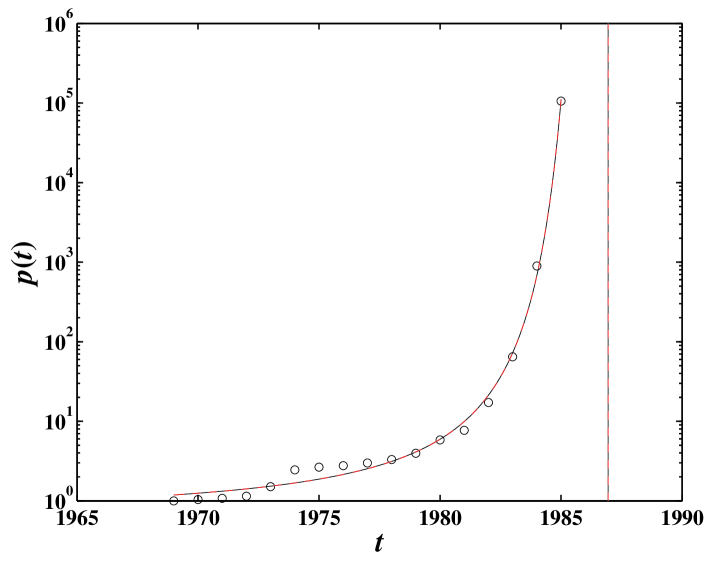
Figure 1: Semi-logarithmic plot of the yearly price index of Bolivia from 1969 to 1985 marked with open circles and its fits with the finite time singular functions (15) (solid line) and (17) (dashed line). The vertical lines indicate the corresponding predicted critical time $t_{c}$.

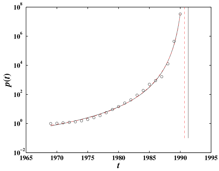
Figure 2: Semi-logarithmic plot of the yearly price index of Peru from 1969 to 1990 marked with open circles and its fits with the finite time singular functions (15) (solid line) and (17) (dashed line). The vertical lines indicate the corresponding predicted critical time $t_{c}$.

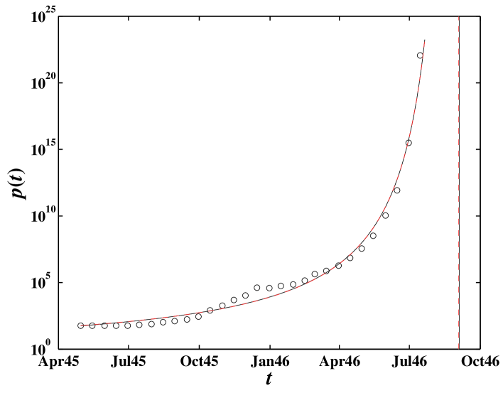
Figure 3: Semi-logarithmic plot of the price index of Hungary from April 30, 1945 to July 31, 1946 marked with open circles and its fits with the finite time singular functions (15) (solid line) and (17) (dashed line). The vertical lines indicate the corresponding predicted critical time $t_{c}$.

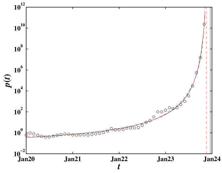
Figure 4: Semi-logarithmic plot of the price index of Germany from January 1920 to November 1923 marked with open circles and its fits to the finite time singular functions (15) (solid line) and (17) (dashed line). The vertical lines indicate the corresponding predicted critical time $t_{c}$.

The hyperinflations of Bolivia, Peru, Hungary and Germany are well fitted by expressions (15) (continuous lines) and (17) (dashed lines) as shown in Figs. 1, 2, 3 and 4, respectively. The parameters of the fits with formulas (15) and (17) to the hyperinflation price time series of the four countries Bolivia, Peru, Hungary and Germany are given in Table 1. There are very small differences between the fits obtained with expressions (15) and (17), suggesting that the considered time intervals are fully in the inflationary expectation regime with strong positive feedbacks. In particular, the exponents $\alpha$ are very robust and the critical times $t_{c}$ are unchanged between the two formulas for Bolivia and Hungary, while $t_{c}$ is moved by two weeks for Germany and by four months for Peru. We also tested the robustness of these results by restricting the fits with to the two formulas (15) and (17) to the last half of each time series. We find that the exponents $\alpha$ and critical times $t_{c}$ are essentially unchanged for the two most dramatic hyperinflation of Hungary and Germany, while $t_{c}$ is pushed forward in the future for Bolivia (by a few years) and Peru (by a few months), without significant degradation of the quality of the fits. This shows that only for Hungary and Germany can one ascertain the critical time of the finite-time singularity with good precision.

In the case of Hungary, the hyperinflation was eventually stopped by the introduction of the present Hungary currency, the Forint, in July 1946. Our prediction of the critical time $t_{c}$ at the beginning of September 1946 suggests that an action on the part of the government was unavoidable as the hyperinflation was close to its climax.

3.2 Evidence of a finite-time singularity regime in $p(t)$ and not in $\ln p(t)$

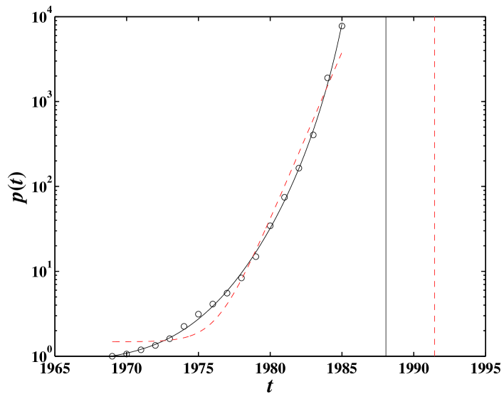
Figure 5: Semi-logarithmic plot of the yearly price index of Israel from 1969 to 1985 marked with open circles and its fits to the right-hand-side of expressions (15) (solid line) and of (17) (dashed line).

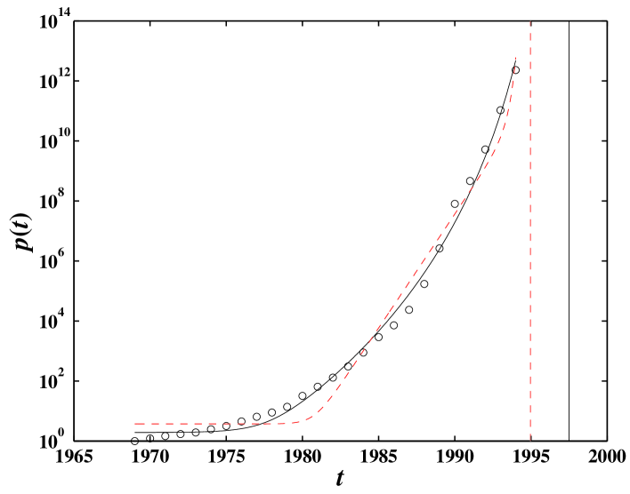
Figure 6: Semi-logarithmic plot of the yearly price index of Brazil from 1969 to 1994 marked with open circles and its fits to the right-hand-side of expressions (15) (solid line) and (17) (dashed line).

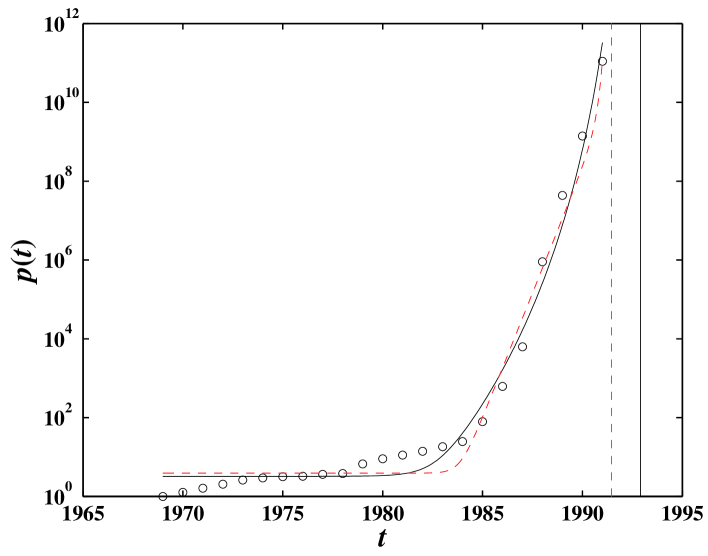
Figure 7: Semi-logarithmic plot of the yearly price index of Nicaragua from 1969 to 1991 marked with open circles and its fits to the right-hand-side of expressions (15) (solid line) and (17) (dashed line).

The cases of Israel, Brazil and Nicaragua are not as clear-cut. While the hyperinflation of these countries clearly exhibited a faster than exponential growth as can be seen from the upward curvature of the logarithm of the price as a function of time in Figs. 5-7, a fit of the price index time series with expressions (15) and (17) give an exponent $\alpha$ larger than $15$ and critical times $t_{c}$ in the range $2020-2080$, which are un-realistic. The results are not improved by reducing the time intervals over which the fits are performed. The results are not improved either by using the alternative formula (16) valid for $m>2$ for which the singularity is weaker as it occurs only on the slope of the log-price.

It is possible that these problems stem from the fact that the latter prices close to the end of the time series start to enter a cross-over to a saturation, as would be expected due to finite-size and rounding effects. Indeed, close enough to the mathematically predicted singularity, one expects that the realized price indexes will eventually saturate and the price dynamics will enter another regime. We believe that it is the start of this regime that makes difficult our recovery of the parameters of expressions (15) and (17). In other words, the problem is not the difference between (15) and (17) capturing a non-critical regime at early times but rather a cross-over to a saturation of the singularity at the latest times.

Since we do not have a theory describing the saturation of the super-exponential growth, we resort to the trick of fitting $p(t)$ rather than $\ln p(t)$ with the right-hand-sides of expressions (15) and (17). This procedure can be seen as the continuous ODE formulation of the double-exponential description of the price index growth advocated by Mizuno et al. [7]. The results are shown in Figs. 5, 6, 7 and Table 2. Notice that, in contrast with the previous cases of Bolivia, Peru, Hungary and Germany, the characteristic cross-over time $\tau$ is rather small, signaling the existence of a significant non-critical regime at early times. For Israel, the fit of the price index $p(t)$ with the right-hand-side of Eq. (17) fails since it has a much larger fit error $\chi=0.348$ than that $\chi=0.085$ of the fit using Eq. (15) and the estimated $t_{c}=1991.44$ is too far off compared with $t_{c}=1988.06$ for the fit of (15).

4 Conclusion

We have presented a novel analysis extending the recent work of Mizuno et al. [7] who analyzed the hyperinflations of Germany (1920/1/1-1923/11/1), Hungary (1945/4/30-1946/7/15), Brazil (1969-1994), Israel (1969-1985), Nicaragua (1969-1991), Peru (1969-1990) and Bolivia (1969-1985). On the basis of a generalization of Cagan’s model of inflation based on the mechanism of “inflationary expectation” or positive feedbacks between realized growth rate and people’s expected growth rate, Mizuno et al. [7] have proposed to describe the super-exponential hyperinflation by a double-exponential function. Here, we have extended their reasoning by noting that the double-exponential function is nothing but a discrete time-step approximation of a more general nonlinear ODE formulation of the price dynamics which exhibits a finite-time singular behavior. In this framework, the double-exponential description is undistinguishable from a power law singularity, except close to the critical time $t_{c}$. Our new extension of Cagan’s model, which makes natural the appearance of a critical time $t_{c}$, has the advantage of providing a well-defined end of the clearly unsustainable hyperinflation regime. We have calibrated our theory to the seven price index time series mentioned above and find an excellent and reliable agreement for Germany (1920/1/1-1923/11/1), Hungary (1945/4/30-1946/7/15), Peru (1969-1990) and Bolivia (1969-1985). For Brazil (1969-1994), Israel (1969-1985) and Nicaragua (1969-1991), we think that the super-exponential growth is already contaminated significantly by the existence of a cross-over to a stationary regime and the calibration of our theory to these data sets has been more problematic. Nevertheless, by a simple change of variable from $\ln p(t)$ to $p(t)$, we obtain reasonable fits, but with much less predictive power. The evidence brought here of well-defined power law singularities reinforces the concept that positive nonlinear feedback processes are important mechanisms to understand financial processes, as advocated elsewhere for financial crashes (see Ref. [8] and references therein) and for population dynamics [4, 10].

Acknowledgments

We acknowledge stimulating discussions with Mr. Takayuki Mizuno. This work was partially supported by the James S. Mc Donnell Foundation 21st century scientist award/studying complex system (WXZ and DS).

Table 1: Parameters of the fits with formulas (15) and (17) as indicated in the first column to the hyperinflation price time series of the four countries Bolivia, Peru, Hungary and Germany. The price indices entered a crossover regime after the end of each period except for Hungary whose hyperinflation of the Pengo was stopped artificially by the introduction of the Forint in July 1946. $\chi$ denotes the root-mean-square residue of the mean-square fits. The price index $p(t)$ for Bolivia and Peru is normalized to $p(1969)=1$ at the beginning of 1969. For Hungary, the time series is the price index. For Germany, it is the exchange rate between the Mark and the US dollar.

Country	Period	$t_{c}$	$\alpha$	$\tau$	$A$	$B$	$\chi$
Bolivia (15)	1969-1985	1986.94	1.3	/	-0.48	29.0	0.204
Bolivia (17)	1969-1985	1986.94	1.3	1000	-0.49	0.068	0.205
Peru (15)	1969-1990	1991.29	0.3	/	-14.17	34.0	0.291
Peru (17)	1969-1990	1990.70	0.01	22.03	-12050	12059	0.283
Hungary (15)	1945/04/30-46/07/15	46/09/03	1.0	/	-1.02	2370	1.168
Hungary (17)	1945/04/30-46/07/15	46/09/03	1.0	1000	-1.68	2.69	1.177
Germany (15)	1920/01/01-23/11/01	23/12/18	0.6	/	-5.09	272	0.490
Germany (17)	1920/01/01-23/11/01	23/12/01	0.3	945	-15.8	14.5	0.459

Table 2: Parameters of the fits of the price index $p(t)$ (and not of $\ln p(t)$) by the right-hand-side of formulas (15) and (17) as indicated in the first column to the hyperinflation price time series of the three countries Israel, Brazil and Nicaragua. The price indices entered a crossover regime after the end of each period. $\chi$ denotes the root-mean-square residue of the mean-square fits. The price index $p(t)$ of each country is normalized to $p(1969)=1$ at the beginning of 1969.

Country	Period	$t_{c}$	$\alpha$	$\tau$	$A$	$B$	$\chi$
Israel (15)	1969-1985	1988.06	5.7	/	0.78	5.10E6	0.085
Israel (17)	1969-1985	1991.44	2.3	2.20	-2.84E5	2.84E5	0.348
Brazil (15)	1969-1994	1997.50	16.3	/	1.93	3.66E21	0.604
Brazil (17)	1969-1994	1994.97	18.6	1.14	-5.77E9	5.77E9	1.196
Nicaragua (15)	1969-1991	1992.91	14.9	/	3.24	4.91E15	0.848
Nicaragua (17)	1969-1991	1991.46	9.2	0.69	-8.03E8	8.03E8	0.945

References

- [1] P. Cagan, The monetary dynamics of hyperinflation, in Milton Friedman (Ed.), Studies in the Quantity Theory of Money (University of Chicago Press, Chicago, 1956).
- [2] P. de Grauwe and M. Polan, Is Inflation Always and Everywhere a Monetary Phenomenon?
- [3] R.T. Froyen and R.N. Waud, The Determinants of Federal Reserve Policy Actions: A Reexamination, Journal of Macroeconomics 24 (3), Summer (2002).
- [4] K. Ide and D. Sornette, Oscillatory Finite-Time Singularities in Finance, Population and Rupture, Physica A 307, 63-106 (2002).
- [5] A. Johansen and D. Sornette, Critical ruptures, Eur. Phys. J. B 18, 163-181 (2000).
- [6] A. Johansen and D. Sornette, Finite-time singularity in the dynamics of the world population and economic indices, Physica A 294, 465-502 (2001).
- [7] T. Mizuno, M. Takayasu and H. Takayasu, The mechanism of double-exponential growth in hyperinflation, Physica A 308 (2002) 411-419.
- [8] D. Sornette, Why Stock Markets Crash (Critical Events in Complex Financial Systems) Princeton University Press (January 2003).
- [9] D. Sornette and J. V. Andersen, Scaling with respect to disorder in time-to-failure, Eur. Phys. Journal B 1, 353-357 (1998).
- [10] D. Sornette and K. Ide, Theory of self-similar oscillatory finite-time singularities in Finance, Population and Rupture, in press in Int. J. Mod. Phys. C 14 (3) (2003).
- [11] J. Temple, Inflation and growth: stories short and tall, preprint ewp-mac/9811009