On energy and momentum of an ultrarelativistic unstable system

Abstract

We study an electron bunch together with its self-fields from the viewpoint of basic dynamical quantities. This leads to a methodological discussion about the definition of energy and momentum for fully electromagnetic systems and about the relation between covariance of the energy-momentum pair and stability. We show here that, in the case of unstable systems, there is no mean to define, in a physically meaningful way, a total energy-momentum four-vector: covariance of the energy-momentum pair follows from the stability of the system and viceversa, as originally pointed out by Henry Poincaré.

DEUTSCHES ELEKTRONEN-SYNCHROTRON

DESY 02-201

November 2002

I INTRODUCTION

Nearly one hundred years have passed since Abraham and Lorentz calculated their famous expressions for the energy and momentum of a purely electromagnetic, spherically symmetrical distribution of charges ABR1 , LORE . This distribution constitutes an attempt to build a classical model of the electron: according to Lorentz’s initial idea, mass, energy and momentum of the electron could, indeed, be of completely elecromagnetic nature.

Nevertheless, the energy (divided by the speed of light in vacuum, as we will understand through this paper) and momentum of such an electromagnetic electron do not constitute a four-vector. In fact (as Abraham ABR2 pointed out already in 1904 probably, at that time, without a clear understanding of what a four-vector is), in a frame moving with velocity ${\bm{v}}$ with respect to the system rest frame, we have

$$E_{e}=\gamma U^{\prime}(1+1/3\beta^{2})$$ (3)

and

$${\bm{P}_{e}}=4/3\gamma{\bm{v}}U^{\prime}/c^{2},$$ (4)

where the index $e$ indicates the electromagnetic nature of the energy $E_{e}$ and momentum ${\bm{P}_{e}}$, $\gamma$ is the usual Lorentz factor, $\beta$ is the velocity $v/c$ (normalized to the speed of light in vacuum $c$), and $U^{\prime}$ indicates the electromagnetic energy in the electron rest frame JACK ,

$$U^{\prime}=\epsilon_{0}/2\int{\bm{E}^{\prime}}^{2}dV^{\prime},$$ (5)

where $\epsilon_{0}$ is the free space permittivity. $U^{\prime}$ is purely an electrostatic quantity (in this paper the prime will always indicate quantities calculated in the rest frame; therefore ${\bm{E}^{\prime}}$ and $dV^{\prime}$ are, respectively, the electric field and the volume element in the rest frame of the system).

It is worth to mention here that the factor $4/3$ in Eq. (4) and the term proportional to $1/3\beta^{2}$ in Eq. (3) depend on the choice of spherical symmetry made on the charge distribution: had we chosen, for instance, an infinitely long line distribution in the direction of ${\bm{v}}$, we would have found

$$E_{e2}=\gamma U^{\prime}(1+\beta^{2})$$ (6)

and

$${\bm{P}_{e2}}=2\gamma{\bm{v}}U^{\prime}/c^{2},$$ (7)

while, in the case of a line charge oriented perpendicularly to the direction of ${\bm{v}}$,

$$E_{e3}=\gamma U^{\prime}$$ (8)

and

$${\bm{P}_{e3}}=\gamma{\bm{v}}U^{\prime}/c^{2},$$ (9)

which only incidentally, due to the particular choice of the distribution, behaves as a four-vector.

Henry Poincaré solved the problem of the lack of covariance shown in Eq. (3) and Eq. (4) by introducing, in the electron model, energies and momenta of non-electromagnetic nature POIN . These are actually due to non-electomagnetic interactions which keep the electron together. By doing so he strongly related the covariance of energy and momentum with the stability of the system: the electomagnetic energy-momentum pair alone is not a four-vector, but the total energy-momenum pair, accounting for the non-electromagnetic interaction, is a regular four-quantity.

In 1922, Enrico Fermi developed an original, early relativistic approach to the $4/3$ problem FERM ; about forty years later a redefinition of the energy-momentum pair related to Fermi’s work was proposed by Rohrlich ROHL , which leaves untouched the total energy-momentum vector, but splits it into electromagnetic and non-electromagnetic contribution in such a way that covariance is granted for both the electromagnetic and the non-electromagnetic part of the energy-momentum pair.

It is possible to show TEUK , GRIF that the treatments by Poincaré and Rohrlich are not in contradiction.

Nevertheless, the approach by Rohrlich ROHL was sometimes taken (see e.g. ERR1 ) as the proof that stability and covariance are unrelated matters since, upon redefinition, the electromagnetic part alone is a four-vector.

We will show here, that such a conclusion is incorrect. The stability of the system is related to the covariance of the total energy-momentum vector, according to the original work by Poincaré: the redefinition procedure mentioned above is indeed acceptable only in the case one is interested in the total energy-momentum vector of a stable system (i.e. a system whose constituents are and stay at rest in a particularly chosen frame), and not in the separate electromagnetic and non-electromagnetic part. Only in that case the arbitrariness included in the recombination of these two contributions does not affect the equation of motion for the system (which deals, in fact, with the total energy-momentum vector).

Some time ago, we were addressing the problem of describing the transverse self-fields originating within an ultrarelativistic electron bunch moving in a fixed trajectory OURS .

This is a particularly relevant problem in modern particle accelerator physics, in view of the need for very high-peak current, low emittance beams to be used, for example, in self-amplified spontaneous emission (SASE)-free-electron lasers operating in the x-ray regime (see for example SAS1 , SAS2 ): in fact, the good quality of the beam may be spoiled by self-interaction occurring within the bunch.

Besides practical relevance (which stresses how, after one hundred years, pure academical problems become relevant also to applied physics), an electron bunch is also a very good example of an unstable system subject to purely electromagnetic interactions. For such a system, the total energy and the total momentum in any frame, are just of electrodynamical nature. We will show that (according to our previous statement about the relation between stability and covariance) there is no way, in this case, to define the total energy-momentum pair in a covariant way. In fact, in contrast to what happens for stable systems, there is no way to describe the evolution of an unstable system without the knowledge of the (electromagnetic) field theory governing the (self-)interactions between its constituents.

II A PARADOX AND ITS SOLUTION

Let us consider a short electron bunch moving, in a given laboratory frame, in a circular orbit. We can simplify the description of this system accounting only for two electrons which will represent the head and the tail of our bunch.

Imagine that the two particles are moving, initially with the same Lorentz factor $\gamma\gg 1$, in a circular orbit of radius $R$, and separated by a (curvilinear) distance $\Delta s\ll R/\gamma^{3}$.

In this situation the two electrons are near enough to be considered travelling with the same velocity vector: indeed it can be shown SAL1 , that they radiate as a single particle of charge $2e$ ($e$ being the electron charge) up to frequencies much above the synchrotron radiation critical frequency (note that, from a quantitative viewpoint, the expression ”much above” is trivially connected to ”how much” $\Delta s\ll R/\gamma^{3}$). The requirements specified before consist, from a geometrical viewpoint, in assuming that, at the beginning of the evolution, the two particles world-lines are very close: actually, considering our resolution in space equal to $R/\gamma^{3}$, they initially coincide.

This assumption justifies the presence of an inertial frame in which both particles are, with good approximation, at rest during the initial part of their evolution. We will refer to it simply as the rest frame. A quantitative definition of the initial part of the evolution may be given when a choice is made about close to zero are the velocities of the particles in the rest frame. Note that the existence of the rest frame is central for our study because, referring to it, one can easily analyze the energy and momentum of the system constituted by the two particles together with their electromagnetic fields.

By means of a Lorentz transformation, then, we can recover the same quantities in the laboratory frame.

Starting with the study in the rest frame we will refer, separately, to mechanical and electromagnetic quantities.

Obviously, in the rest frame, the mechanical momentum of the system, ${\bm{P}^{\prime}_{ne}}$, is zero, and the mechanical energy, $E^{\prime}_{ne}$, is just equal to $2mc^{2}$, where $m$ is the electron rest mass.

The study of the electromagnetic contributions to energy and momentum is also trivial. Since the electrons are at rest they produce electric field only. Therefore the Poynting vector vanishes and ${\bm{P}^{\prime}_{e}}=0$. On the other hand, $E_{e}$ is given, simply, by the work $U^{\prime}$ done against the field to bring the two particles together (quasistatically) from a situation in which they are separated by an infinite distance.

By doing so, of course, we are neglecting, in both ${\bm{P}^{\prime}_{e}}$ and $E^{\prime}_{e}$, the contributions from the acceleration (self-)fields generated by the system.

This approximation is justified by the fact that we are discussing the asymptotic behavior for the two particles separated by a very small distance: then, as it will be clear from Eq. (18) and Eq. (27), we may assume that the acceleration field contribution are unimportant, when compared with the Coulomb one. In fact acceleration effects saturate in the asymptotic limit of small distance between the two particles SAL1 , while Coulomb ones are singular; once again it must be clear that we are discussing the asymptotic case for small distance between the two particles. Therefore we have:

$$E^{\prime}_{e}=U^{\prime}=e^{2}/(4\pi\epsilon_{0}\gamma\Delta s)$$ (10)

and

$${\bm{P}^{\prime}_{e}}=0.$$ (11)

Summing up the electromagnetic and mechanical contributions one gets the total energy and momentum for the system:

$$E^{\prime}_{tot}=E^{\prime}_{ne}+E^{\prime}_{e}=2mc^{2}+U^{\prime}$$ (12)

and

$${\bm{P}^{\prime}_{tot}}={\bm{P}^{\prime}_{ne}}+{\bm{P}^{\prime}_{e}}=0.$$ (13)

As already said one may, now, use a Lorentz transformation in order to calculate these quantities in the laboratory frame. Again, since we are interested at the beginning of the evolution, it follows from our assumptions that the two particles evolve with the same four-velocity vector. Therefore a direction of motion (which we will designate with z) is well defined for the system in the laboratory frame and the Lorentz transformation from the rest frame is, indeed, a simple boost in the $-z$ direction (note that a good definition of the $z$ direction is equivalent to a good definition of the rest frame). We will represent this boost with a matrix with components $\Lambda^{\mu}_{\ \nu}$ with $\mu,\nu=0...3$ (where the third component corresponds to the $z$ direction):

$$\Lambda^{\mu}_{\ \nu}=\left(\begin{array}[]{cccc}\gamma&0&0&\beta\gamma\\ 0&1&0&0\\ 0&0&1&0\\ \beta\gamma&0&0&\gamma\\ \end{array}\right).$$ (14)

The use one makes of $\Lambda^{\mu}_{\ \nu}$ is a critical point in our derivation. If one (erroneously) assumes that energy and momentum constitute a four-vector, then he gets, straightforwardly:

$$(E_{tot}/c,{\bm{P}_{tot}})^{\mu}=\Lambda^{\mu}_{\ \nu}(E^{\prime}_{tot}/c,{\bm{P}^{\prime}_{tot}})^{\nu}$$ (15)

and, therefore,

$${E_{tot}/c}=\gamma\left(2mc^{2}+U^{\prime}\right),$$ (16)

and

$${P_{tot}}=\gamma\left(2m+U^{\prime}/c^{2}\right)\beta c~{},$$ (17)

where $P_{tot}$ is a scalar quantity, since we understand that ${\bm{P}_{tot}}$ is oriented along the $z$ direction.

We can now project the equation of motion, ${\bm{F}_{syst}}=d{\bm{P}_{tot}}/dt$, onto the transverse direction (perpendicular to $z$ and lying on the orbital plane) thus getting, within our approximations:

$$F_{\mathrm{\bot syst}}=2eB\beta c+{e^{2}\over{4\pi\varepsilon_{\mathrm{0}}R\Delta s}}$$ (18)

As already mentioned in Section I (with in mind the applications in the physics of particle accelerators and the one of SASE-FELs, see SAS1 , SAS2 ) we addressed the description of the transverse self-fields originating within an electron bunch moving in a circle in OURS . In that paper an approach has been proposed which involves purely electrodynamical considerations, based on the retarded Green function solution of Maxwell equations.

In particular, in part of OURS we treated the case of two particles separated by a distance $\Delta s$ (non necessarily much smaller than $R/\gamma^{3}$), moving rigidly in a circle (see Fig. 1) of radius $R$. Our results disagree with Eq. (18).

Let us briefly justify the latter statement. The total transverse force (orthogonal to its velocity and lying on the orbital plane) felt by the head electron and due to the tail electron source turned out to be (see, again OURS ):

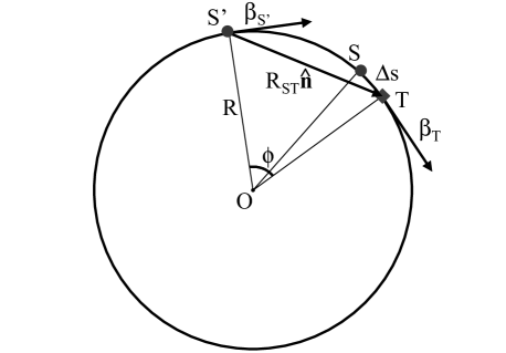
Figure 1: Geometry for the two-particle system in the steady state situation, with the test particle ahead of the source. Here T is the present position of the test particle, S is the present position of the source, while S’ indicates the retarded position of the source.

$${F_{\mathrm{\bot}}}\simeq{e^{2}\gamma^{3}\over{4\pi\varepsilon_{\mathrm{0}}R^{2}}}\Phi(\hat{\phi})~{},$$ (19)

where $\Phi$ is defined by

$$\Phi(\hat{\phi})={2+\hat{\phi}^{4}/8\over{\hat{\phi}(1+\hat{\phi}^{2}/4)^{3}}}~{},$$ (20)

Here $\hat{\phi}$ is the retarded angle $\phi$ (which expresses the angular distance between the retarded position of the source the present position of the test electron, see Fig. 1, normalized to the synchrotron radiation formation angle at the critical frequency, $1/\gamma$, i.e. $\hat{\phi}=\gamma\phi$. Eq. (20) is completely independent of the parameters of the system.

It is straightforward to study the asymptotic behaviors of $\Phi$. In order to do so, just remember that the retardation condition linking $\Delta s$ and $\phi$ is given by (see OURS , SAL1 ):

$$\Delta s=R\phi-2\beta R\sin{\phi\over{2}}~{},$$ (21)

or by its approximated form

$$\Delta s=(1-\beta)R\phi+{R\phi^{3}\over{24}}~{}.$$ (22)

It is now evident that $\Phi(\Delta\hat{s})\rightarrow 1/(3\Delta\hat{s})$ when $\hat{\phi}\gg 1$ and $\Phi(\Delta\hat{s})\rightarrow 1/(\Delta\hat{s})$ when $\hat{\phi}\ll 1$, having introduced the normalized quantity $\Delta\hat{s}=(\gamma^{3}/R)\Delta s$. This normalization choice is, again, linked with the fact that the critical synchrotron radiation wavelength, $R/\gamma^{3}$, is also the minimal characteristic distance of our system: as we said before, two particles nearer than such a distance can be considered as a single one radiating, up to the critical frequency, with charge $2e$ (see OURS , SAL1 ).

The asymptotic behavior above suggests to study the function $\Phi(\Delta\hat{s})\Delta\hat{s}$. We plotted such a function in Fig. 2 (and the contribution from the acceleration field alone) for values of $\Delta\hat{s}$ running from 0 to 5.

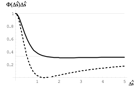
Figure 2: Plot of $\Phi(\Delta\hat{s})\Delta\hat{s}$ (solid line) and comparison with the asymptotic values, $1$ and $1/3$. The dashed line shows the contribution from the acceleration field, $\Phi_{\mathrm{R}}(\Delta\hat{s})\Delta\hat{s}$, alone.

As it is seen from the figure, the contribution from the velocity field is not important in the asymptotic limit for particles very nearby (our case) or very far away. When, in particular, $\Delta s\ll R\gamma^{3}$ we can approximate Eq. (19) by

$${F_{\mathrm{\bot}}}\simeq{e^{2}\over{4\pi\varepsilon_{\mathrm{0}}R\Delta s}}~{}.$$ (23)

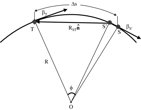
Figure 3: Geometry for the two-particle system in the steady state situation, with the source particle ahead of the test one. Here T is the present position of the test particle, S is the present position of the source, while S’ indicates the retarded position of the source.

On the other hand, as regards the force felt by the tail particle (see Fig. 3), it is easily seen that (see OURS , SAL1 ) the test electron, which now is the tail particle, ”runs against” the electromagnetic signal emitted by the source (while in the previous case it just ”runs away” from it). Therefore the relative velocity between the signal and the test electron is equal to $(1+\beta)c$ (instead of $(1-\beta)c$ in the other situation). Hence the retardation condition reads

$$\Delta s=R\phi+2\beta R\sin{\phi\over{2}},$$ (24)

or, solved for $\phi$ in its approximated form,

$$\phi\simeq{\Delta s\over{R(1+\beta)}}~{}.$$ (25)

In this situation, $\bm{\beta_{\mathrm{S}}}$ is almost parallel (and equal) to $\bm{\beta_{\mathrm{T}}}$ and antiparallel to $\hat{\bm{n}}$ (which is the unit vector oriented as the line connecting the retarded source to the present test particle): it turns out that the only important contribution to the transverse force results from the acceleration field and reads:

$${F_{\mathrm{\bot}}}\simeq{e^{2}\over{4\pi\varepsilon_{\mathrm{0}}R\Delta s}}~{}.$$ (26)

In the case under study, since $\Delta s\ll R/\gamma^{3}$, the total self-force acting on the system is given by the sum of Eq. (23) and Eq. (26):

$${F_{\mathrm{\bot}}}\simeq 2{e^{2}\over{4\pi\varepsilon_{\mathrm{0}}R\Delta s}}~{},$$ (27)

which is in disagreement of a factor $2$ with respect to the self-force term in Eq. (18). In other words, had we erroneously assumed covariance, we would have encountered a paradox. Again, note that we are treating the asymptotic limit of a small distance between the two electrons: in this limit we can neglect the contribution from the acceleration field in the equation of motion Eq. (18). In fact this contribution saturates for small distance between the two particles (see SAL1 ), while the term missing by comparison between Eq. (18) and Eq. (27) is singular (and, therefore, dominating) in the limit when $\Delta s$ goes to zero.

This situation should not be too much surprising for the reader familiar with the works ABR1 … ABR2 which led to Eq. (3) and (4): the derivation of Eq. (18) is, in fact, performed under the explicit assumption that energy and momentum constitute a four-vector.

As we will immediately see, in the case of unstable systems (like the one we deal with), the use of correct transformation laws for the electromagnetic stress tensor solves the problem but spoils the covariance of the energy-momentum pair.

The energy and momentum of an electromagnetic system in the laboratory frame is given by

$$E=\int T^{\prime\mu\nu}\Lambda^{0}_{\ \mu}\Lambda^{0}_{\nu}{dV^{\prime}\over{\gamma}}$$ (28)

$$P^{i}={1\over{c}}\int T^{\prime\mu\nu}\Lambda^{i}_{\ \mu}\Lambda^{0}_{\ \nu}{dV^{\prime}\over{\gamma}},$$ (29)

where $T^{\mu\nu}$ are the components (in the rest frame) of the electromagnetic stress tensor of the system, which contains all the information about the (electromagnetic) field theory governing the interactions between the particles. The process of lowering and raising indexes is governed in the usual way by the metric tensor. Here the latin index $i$ runs from 1 to 3 and, as already said, the quantities with prime refer to the rest frame. In our case we will consider the only important component, i.e. the third (along $z$).

Note that the integrals in Eq. (28) and Eq. (29) include both a single-particle term and an interaction term (compare also GRIF ). Here we are interested in the interaction term alone: in fact we will treat the (trivial) mechanical contributions to the energy-momentum pair separately and, once again, we will neglect the acceleration-field contributions. Therefore, in the following, we will understand that $T^{\prime}$ refers to the interaction term alone.

Then, since the mechanical energy-momentum pair of a single particle is a 4-vector, one gets:

$$(E_{ne}/c,P_{ne})^{\mu}=\Lambda^{\mu}_{\ \nu}(E^{\prime}_{ne}/c,P^{\prime}_{ne})^{\nu}~{},$$ (30)

hence

$$E_{ne}=2\gamma mc^{2}$$ (31)

and

$$P_{ne}=2\beta\gamma mc.$$ (32)

while

$$E_{e}=\beta^{2}\gamma\int T^{\prime 33}dV^{\prime}+\gamma U^{\prime},$$ (33)

$$P_{e}=\gamma\beta U^{\prime}/c+\gamma\beta/c\int T^{\prime 33}dV^{\prime},$$ (34)

We should note, here (but this is a valid methodological remark also as regards the previous, incorrect approach), that the particles are subject to a long-range interaction (the electromagnetic interaction) and, therefore, a covariant definition of the total energy and momentum is not straightforward even when one is considering the two particles alone, without including (as we did, instead) the electromagnetic fields in the system. Therefore, strictly speaking, one may object that Eq. (30) does not make any sense at all.

Indeed, if the interaction occurred at a single point in space-time (short-range scattering case), the particle velocities would have been constant, in the view of any inertial observer, before and after the scattering took place. Then if two observers related by a Lorentz boost compared their judgments about the particles velocities, they would have found that these are linked by a Lorentz transformation, the same which transforms from one observer to the other. Nevertheless, this is a particular case. We must remember that, in general, according to the Theory of Relativity, the concept of simultaneity depends on the observer. Therefore, when (as in the situation under study) one deals with a long-range interaction, the velocities of the particles, in the judgment of the two observers above, are not related by a Lorentz transformation anymore (see TRUM ): the objection about the correct definition of the mechanical energy-momentum vector follows directly from this observation. A good definition of the energy-momentum vector of the two-particle system alone (without their fields!) can, in fact, be recovered using more subtle geometrical methods only, like a regular correlated representation of the world lines (see TRUM ).

However this objection does not concern us, here, since, as already implicit in the definition of the $z$ direction, we discuss about that region of space-time in which the two particles world lines are very close and are roughly characterized by the same Lorentz factor, that is, once again, at the beginning of the evolution.

Then we can use Eq. (30)… Eq. (34) to get, by summation, the total energy and momentum of the system in the laboratory frame and in the direction of motion (see also JACK and MOLL ):

$${E_{tot}}=\gamma\left(2mc^{2}+U^{\prime}+\beta^{2}\int T^{\prime 33}~{}dV^{\prime}\right),$$ (35)

and

$${P_{tot}}=\gamma\left(2m+U^{\prime}/c^{2}+{1\over{c^{2}}}\int T^{\prime 33}~{}dV^{\prime}\right)\beta c~{}.$$ (36)

Note that Eq. (35) and Eq. (36) can be used to obtain Eq. (3) and Eq. (4), as well as Eq. (6)… Eq. (9): different distributions of charge give different expressions for the electromagnetic stress tensor and for the electromagnetic energy.

In our case of two electrons we already know the explicit expression for $U^{\prime}$. In fact we remind that, as has already been said, the electromagnetic interaction energy is simply given by the work done against the field to bring the two particles together, quasistatically, from a situation in which they are separated by an infinite distance:

$$U^{\prime}\simeq{e^{2}\over{4\pi\varepsilon_{\mathrm{0}}\gamma\Delta s}}~{}.$$ (37)

On the other hand it is easy to calculate $T^{\prime\mathrm{}}{33}$ (in the rest frame, since we need to integrate over $V^{\prime}$). To this purpose we remind that, in the rest frame (and at short distance $\gamma\Delta s\ll R/\gamma^{2}$, so that the acceleration field contributions are unimportant), the space-space components of the total (comprehensive of both single particle and interaction part) symmetric energy-momentum tensor read (see JACK ):

$$T^{\prime ij}_{tot}=-\varepsilon_{0}(E^{\prime}_{i}E^{\prime}_{j}-\delta_{ij}E^{\prime 2}/2)~{},$$ (38)

where, here, i, j = 1.. 3. The discussion above shows that, for us, the only interesting component is $T^{\prime}_{33}$. It can be proven that the interaction part alone is just

$$\int T^{\prime 33}~{}dV^{\prime}=U^{\prime}~{}.$$ (39)

Note that Eq. (39) describes also the case of a charged line distribution oriented in the direction of motion (in the case of a charged line, of course, the single-particle term is not present at all).

The equations for the energy and momentum of the system in the laboratory frame now read:

$${E_{tot}}=\gamma\left[2mc^{2}+U^{\prime}(1+\beta^{2})\right]$$ (40)

and

$${P_{tot}}=\gamma\left(2m+2U^{\prime}/c^{2}\right)\beta c~{},$$ (41)

whose electromagnetic parts are the same of Eq. (6) and Eq. (7).

From the transverse component of the equation of motion for the system one gets

$$F_{\mathrm{\bot syst}}\simeq 2eB\beta c+2{e^{2}\over{4\pi\varepsilon_{\mathrm{0}}R\Delta s}}$$ (42)

Eq. (42) is now in perfect agreement with our result in Eq. (27).

Both the terms on the right hand side of Eq. (42) are centripetal as well as in Eq. (18) (although, of course, Eq. (18) and Eq. (42) are in disagreement as concerns the magnitude of the self-interaction term); the first describes the motion of the system under a magnetic field, while the second is linked with the presence, in the system, of electromagnetic fields: an extra centripetal (external) force is needed, if one wants to keep the system moving in a circle of radius $R$, compensating for the centrifugal self-field contributions calculated in OURS .

III DISCUSSION

In order to reach the agreement between Eq. (42) and Eq. (27), one has to give up the covariance of the energy-momentum pair of our system, as it is seen directly from Eq. (40) and Eq. (41).

We can sum up the discussion in Section II by saying that the assumption of covariance for the transformation of the energy-momentum pair of an unstable system leads to a paradox. Such a paradox can be solved introducing the correct transformation laws for the energy-momentum tensor. In this way, it is seen that the energy-momentum pair for an unstable system (particles and electromagnetic field) is not a four-vector. We already mentioned in Section I, that the non-covariant character of energy and momentum is also present when one discusses some classical problems which involve the relativistic dynamics of a charged particles stable system. Nevertheless, in these cases, covariance can be always restored by introducing non-electromagnetic stresses which keep the system together or, equivalently, by redefinition (see ROHL ) of the energy-momentum pair. In particular we can refer to the $4/3$ problem in the classical electron model (as done above in Section I) but also to other problems like, for example, the explanation of the Trouton-Noble paradox, which has been treated extensively in literature (see TEUK , TRA1 .. BUTL ) all over the last century.

As we already said in Section I, there is one major difference with respect to our case, though: our system, in contrast with the latter ones, is, by nature, unstable; there is no reference frame such that its components are and stay at rest. This fact leads to a major difference in the treatment of the total energy and momentum.

In the case of a stable system, the total energy and momentum of the system (including non-electromagnetic binding forces) constitute a four-vector, a well-defined geometrical entity.

On the contrary, in the case of an unstable system, this pair of quantities has no geometrical meaning, although it is possible to give, of course, separate definitions of total energy and momentum in the judgment of any observer.

In the situation discussed in Section II this is a direct consequence of the fact that we deal with a fully electrodynamical system and there is no way to introduce, in a straightforward way, an analogue of Poincaré stresses. As a result we must conclude that stability of the system and covariance of the energy-momentum pair are bound together.

Let us discuss the latter statements in detail, starting with a review of well-known arguments for stable systems.

Stable systems are characterized by a zero (total self-) four-force density. When the four-force density can be derived from an energy-momentum tensor $T^{\mu\nu}$, the latter property is equivalent to:

$$T^{\mu\nu}_{\ \ \ ;\mu}=0~{},$$ (43)

which is the requirement for a zero-divergency energy-momentum tensor.

However, Eq. (43) refers to the total energy-momentum tensor, while the electromagnetic part of it is not divergenceless at all (its divergence is, simply, the Lorentz four-force density).

On the other hand, since stability is characterized by a zero total four-force density, non-electromagnetic stresses must be present (Poincaré stresses), which balance the Lorentz four-force density, thus insuring stability for the system. Poincaré stresses also insure covariance for the energy-momentum pair which is, therefore, a well-defined four-vector: to prove this, one can remember the definition of the total energy-momentum pair (see JACK , TEUK ):

$$P^{\mu}={1\over{c}}\int_{\sigma}T^{\mu\nu}d\sigma_{\nu}$$ (44)

where the integration is carried out over any hypersurface at $t=constant$ (actually $\sigma$ may be, more generally, any spacelike surface, see TEUK ) for any inertial observer.

It can be easily proved (see TEUK ) that Eq. (44) is independent from the choice of the integration hypesurface. Such a proof is based on Eq. (43).

The choice of different inertial observers is equivalent to the choice, on the space-time manifold, of different time-like unit vectors. The different families of hypersurfaces orthogonal to these vectors represent the physical space at a certain time in the judgement of different observers. From the independence of the definition in Eq. (44) of the choice of the integration hypersurface follows, therefore, the independence of $P^{\mu}$ on the reference frame used to evaluate it, and this constitutes the proof that $P^{\mu}$ is a well-defined four-vector.

Since $P^{\mu}$ is independent from the choice of the integration hypersurface, one is free to choose the one which helps better in solving problems. Historically, two choices have been used in explaining, for example, the Trouton-Noble paradox. The first (see TEUK ) consists in considering the surface at $t=constant$ for any observer. This leads to the usual expressions for the electromagnetic energy and momentum in a given frame:

$${E_{e}\over{c}}=P^{0}_{e}={1\over{2c}}\int\left(\epsilon_{0}{\bm{E}}^{2}+{{\bm{B}}^{2}\over{\mu_{0}}}\right)dV$$ (45)

and

$${\bm{P}_{e}}={1\over{\mu_{0}c^{2}}}\int\left({\bm{E}}\times{\bm{B}}\right)dV,$$ (46)

where $\mu_{0}$ is the free space permeability.

While Eq. (45) and Eq. (46) do not constitute a four-vector, one can straightforwardly solve the problem of the lack of covariance by introducing Poincaré stresses.

The second choice consists in selecting $t=constant$ in the rest frame of the system:

$${E_{e}\over{c}}=P^{0}_{e}={1\over{c}}\int\left[{1\over{2}}\left(\epsilon_{0}{\bm{E}}^{2}+{{\bm{B}}^{2}\over{\mu_{0}}}\right)-{\bm{v}}\cdot{{\bm{E}}\times{\bm{B}}\over{\mu_{0}c^{2}}}\right]dV$$ (47)

and

$${\bm{P}_{e}}={\gamma\over{c}}\int\Big{[}{{\bm{E}}\times{\bm{B}}\over{\mu_{0}c}}-{{\bm{v}}\over{2}}\cdot\left(\epsilon_{0}{\bm{E}}^{2}+{{\bm{B}}^{2}\over{\mu_{0}}}\right)+$$

$$+\epsilon_{0}({\bm{v}}\cdot{\bm{E}}){\bm{E}}+({\bm{v}}\cdot{\bm{B}}){{\bm{B}}\over{\mu_{0}}}\Big{]}dV$$ (49)

In this case it can be easily shown (see ROHL , TEUK ) that the electromagnetic part of the total energy-momentum pair is, actually, a four-vector. This is, in fact, the same redefinition of the four-momentum that Rohrlich used to deal with the electron problem ROHL . One can easily check (see TEUK ) that, in this case, the non-electromagnetic part of the total energy-momentum pair is zero.

All this illustrates the well-known fact that the introduction of Poincaré stresses or the Rohrlich redefinition of energy and momentum are, in fact, equivalent in essence. The choice of the integration hypersurface is a matter of taste for stable systems, since the only important quantity from a geometrical viewpoint is the total energy-momentum four-vector, given by the sum of the electromagnetic and the non-electromagnetic part; this sum, by definition, is independent from such a choice. In other words, different choices of the hypersurface just split the same, total quantity onto two parts (electromagnetic and non-electromagnetic) in two distinct ways but, as quoted from TEUK : ”The split into electromagnetic and non-electromagnetic parts is quite arbitrary”.

Our point is that this situation is completely different in the case of unstable systems, where only electromagnetic forces are present and Poincaré stresses are not.

In the case of unstable systems there is no way one can define the total energy-momentum four-vector. This statement is justified, from a mathematical viewpoint, by the fact that

$$T_{tot\ ;\mu}^{\mu\nu}=T_{e\ \ \ ;\mu}^{\mu\nu}\neq 0~{};$$ (50)

in fact, from the previous discussion, we know that divergenceless is an essential ingredient for the independence of the total energy-momentum pair from the choice of the integration hypersurface.

Note that Eq. (50) means that there is a non-vanishing four-force density field over the space-time. In the case discussed in Section II we gave a practical example of the latter statements.

Of course, also for unstable systems, we may consider an observer and find out the energy and momentum of the system with respect to that observer, but this quantities will not be covariant, nor we can recover covariance by integrating the energy-momentum tensor over a suitable hypersurface (as done with stable systems), since the electromagnetic energy-momentum pair (which coincides now with the total energy-momentum pair) would change Eq. (40) and Eq. (41), thus giving an unphysical result on the second term of Eq. (42), when compared with Eq. (27). The latter discrepancy, to the authors view, is similar to the one encountered in GRIF . In that paper a system composed by two electron is studied too and a comparison is proposed between energy-derived mass $m_{u}$ (electrostatic energy divided by $c^{2}$), momentum derived mass $m_{p}$ (momentum divided by $\gamma v$, being $v$ the system velocity) and self-force-derived mass $m_{s}$ (self-force divided by $\gamma^{3}a$, $a$ being the system acceleration). The authors of GRIF point out that $m_{s}=m_{p}\neq m_{u}$ and that the inequality between $m_{p}$ and $m_{u}$ can be solved by redefining, following Rohrlich (see ROHL ) the energy-momentum pair. Nevertheless, in this case, one is left with a discrepancy between $m_{s}$ and $m_{u}$. This fact is perceived by the authors of GRIF as an unsolved paradox. Actually the derivation of Eq. (18) (or equivalently, of $m_{u}$, treated with Rohrlich’s method) is performed under the explicit assumption that energy and momentum constitute a four-vector which is true only in the case of a stable system. As a result, by comparing Eq. (18) and Eq. (27) or, which is the same, $m_{u}$ (treated by Rohrlich’s method or, equivalently, by introducing Poincaré stresses) with $m_{s}$, one is comparing quantities which refer to a stable system with quantities which refer to an unstable one, thus giving a paradoxical result.

Consider, as a last example, an unstable system formed by different subsystems initially at rest in a certain frame (as in the case discussed in Section II). In general, while dealing with unstable systems, the knowledge of dynamical quantities for the subsystems cannot bring any information about the behavior of the system as a whole, unless we have knowledge of the (electromagnetic) field theory governing the interactions (which make the system unstable).

In our example of Section II, even if we can measure, in a certain frame, the particle velocities when they are far away from each other (thus no more interacting) and if we know their rest masses, we cannot say anything about energy and momentum of the total system without the knowledge of the stress tensor, and the reason for that is the presence of a non-zero four-force density field (which we can account for only knowing the stress tensor, i.e. the interaction theory) on that part of the four-dimensional manifold on which we want to have information.

Suppose our system was stable (think about an ideal ”rope” responsible for Poincaré stresses, or think, instead of the case of two electrons, about a nuclear fission process in which electromagnetic fields are, before the fission event, balanced by the strong interaction). Put ourselves in the laboratory frame, and imagine that, at a certain moment, for a certain reason (a collision with a neutron, for example) the Poincaré stresses are not present anymore. Thus the system becomes unstable, it breaks in two subsystems and the electromagnetic interaction (if you’re thinking about the nucleus imagine we are talking about a charged ion) takes over. If we wait for enough time the two particles will get far away from each other and we can consider them no more interacting.

At this point, the kinetic energy of the particles is equal to the energy previously stored in the electromagnetic field when the system was stable: thus we are able to get information about the total energy-momentum vector of the stable system even if we do not know anything about the stress tensor and the theory of the interaction between the subsystems. In fact, the sum of the momenta of the two free particles and the sum of their energies will give us, respectively, the energy and the momentum of the stable system, which form a four-vector again.

The reason is, simply, that there is no four-force density field in that part of the space time on which we want to have information: from a general viewpoint we can conclude that the presence of a four-force density, which characterizes unstable systems, spoils without remedy the covariance of the energy-momentum pair. The only way to recover such covariance would be to introduce a balancing four-force density, i.e. to make the system stable.

In other words, in agreement with Poincaré, from the stability of the system follows the covariance of the system and, vice versa, from covariance follows stability: the energy-momentum pair of an unstable system does not constitute a four-vector. This conclusion may seem, at first glance, of academical importance only. It has, indeed, very practical consequences in modern electron beam physics. Energy and momentum of an electron bunch are physically measurable quantities and an electron bunch itself is a practical example of an unstable system. Nowadays, technology allows the production of ultra high-brightness, intense electron beams (to be used, for example, in self-amplified spontaneous emission (SASE)-free-electron lasers operating in the x-ray regime). The production of such bunches is one of the most challenging activities for particle accelerators physicists. The description of these systems would be completely incorrect without accounting for self-interactions in the right way. We can conclude that, for example, simulation codes (as well as analytical considerations: actually, as already reminded, we wrote this paper after studying the self-interactions within an electron bunch) which rely on the covariance of the energy-momentum pair would give, $a\ priori$, wrong results which may be immediately confuted by experimental control. Technological developments often transform, as in this case, purely methodological issues into very practical ones.

IV ACKNOWLEDGEMENTS

The authors acknowledge Reinhard Brinkmann, Georg Hoffstaetter, Martin Dohlus, Helmut Mais and Evgeni Schneidmiller (DESY), Yaroslav Derbenev, Rui Li and Yuhong Zhang (Jefferson Lab), Mikhail Yurkov (JINR), Jan Botman, Jom Luiten and Marnix van der Wiel (Technische Universiteit Eindhoven) with useful discussions. Moreover G.G. greatly appreciates financial support from the Centrum voor Plasmafysica en Stralingstechnologie (CPS, the Dutch Centre for Plasma Physics and Radiation Technology) and both financial support and hospitality granted by the Center for Advanced Studies of Accelerators (CASA) at Thomas Jefferson National Laboratory during his work on this paper.

References

- (1) M. Abraham, Theorie der Elektrizitat, vol II: Elektromagnetische Theorie der Stralung, Teubner, Leipzig, 1905
- (2) H.A. Lorentz, The Theory of electrons, Leipzig, Teubner, 1909
- (3) M. Abraham, Phys. Z., 5, 1904
- (4) J. D. Jackson, Classical Electrodynamics, Wiley, N.Y.
- (5) H. Poincaré, On the dynamics of the electron, Rendiconti del Circolo Matematico di Palerma 21, 129, 1906
- (6) E. Fermi, Il Nuovo Cimento, 25, 159-170, 1923
- (7) F. Rohrlich, Classical Charged Particles (Addison-Wesley, Reading, Mass., 1965), Sec. 6-3
- (8) S. A. Teukolsky, Am. J. Phys. 64 (9), 1104, 1996
- (9) D. J. Griffiths and R. E. Owen, Am. J. Phys. 51 (12), 1120, 1983
- (10) M. H. Mac Gregor, The enigmatic electron (Kluwer Academic Publishers, Dordrecht /Boston/London, edited by Alwyn van der Merwe), pp. 19-24
- (11) G. Geloni et al., DESY 02-048, May 2002; also, to be submitted to Phys. Rev. E
- (12) TESLA Technical Design Report, DESY 2001-011, edited by F. Richard et al. and http://tesla.desy.de/
-
(13)
The LCLS Design
Study Group, LCLS Design Study Report, SLAC reports SLAC -R521,
Stanford (1998)
and http://www-ssrl.slac.stanford.edu/lcls/CDR - (14) E. L. Saldin, E. A. Schneidmiller and M. V. Yurkov, Nucl. Instr. Methods A 398, 373 (1997)
- (15) M.A. Trump at al., Classical Relativistic Many-Body Dynamics, Kluwer Academic Publishers, Dordrecht, 1999
- (16) C. Möller, The theory of relativity, second edition, Chapter 7, Clarendon press, Oxford (1972)
- (17) M. v. Laue, Ann. Phys. 35, 524, 1911
- (18) W. Pauli, The thory of relativity, (Pergamon, New York, 1958)
- (19) A. K. Singal, Am. J. Phys. 61, 428, 1993
- (20) J. W. Butler, Am. J. Phys. 36, 936, 1968