Intermittency, scaling and the Fokker-Planck approach to
fluctuations of the solar wind bulk plasma parameters as seen by
the WIND spacecraft.

Abstract

The solar wind provides a natural laboratory for observations of MHD turbulence over extended temporal scales. Here, we apply a model independent method of differencing and rescaling to identify self-similarity in the Probability Density Functions (PDF) of fluctuations in solar wind bulk plasma parameters as seen by the WIND spacecraft. Whereas the fluctuations of speed $v$ and IMF magnitude $B$ are multi-fractal, we find that the fluctuations in the ion density $\rho$, energy densities $B^{2}$ and $\rho v^{2}$ as well as MHD-approximated Poynting flux $vB^{2}$ are mono-scaling on the timescales up to $~{}26$ hours. The single curve, which we find to describe the fluctuations PDF of all these quantities up to this timescale, is non-Gaussian. We model this PDF with two approaches– Fokker-Planck, for which we derive the transport coefficients and associated Langevin equation, and the Castaing distribution that arises from a model for the intermittent turbulent cascade.

I Introduction

Statistical properties of velocity field fluctuations recorded in wind tunnels and these obtained from solar wind observations exhibit striking similarities carbone (1, 2). A unifying feature found in these fluctuations is fractal or multi-fractal scaling. The Probability Density Function (PDF), unlike power spectra that do not reveal intermittency, show a clear departure from the Normal distribution when we consider the difference in velocity on small spatial scales bohr (3, 4) while large scale features appear to be uncorrelated and converge toward a Gaussian distribution. These similarities suggest a common origin of the fluctuations in a turbulent fluid and the solar wind. The approach is then to treat the solar wind as an active highly nonlinear system with fluctuations arising in situ in a manner similar to that of hydrodynamic turbulence cytu (5, 6, 7, 8).

Kolmogorov’s K41 turbulence theory was based on the hypothesis that the energy is transferred in the spectral domain at a constant rate through local interaction within the inertial range. This energy cascade is self-similar due to the lack of any characteristic spatial scale within the inertial range itself. These assumptions led Kolmogorov to his scaling law for the moments of velocity structure functions frisch (4): $S_{\ell}^{n}=\left<|v(r+\ell)-v(r)|^{n}\right>\propto(\epsilon\ell)^{n/3}$, where $n$ is the $n$-th moment, $\ell$ is a spatial scale and $\epsilon$ represents energy transfer rate. Experimental results do not confirm this scaling, however, and modifications to the theory include intermittency k62 (9) by means of a randomly varying energy transfer rate $\epsilon$. In this context, empirical models have been widely used to approximate the shapes of fluctuation PDFs of data from wind tunnels castaing (10) as well as the solar wind; see for example valvo (11, 12). The picture of turbulence emerging from these models is much more complex then has been suggested by the original Kolmogorov theory. It requires a multi-fractal phenomenology to be invoked as the self-similarity of the cascade is broken by the introduction of the intermittency.

Recently, however, a new approach has emerged where the presence of intermittency in the system coincides with statistical self-similarity, rather than multi-fractality, in the fluctuations of selected quantities; these also exhibit leptokurtic PDFs. An example of this statistical intermittency was discussed in mantegna95 (13), where a Lévy distribution was successfully fitted to the fluctuation PDFs of the price index over the entire range of data. Such a distribution arises from the statistically self-similar Lévy process also characterized by enhanced (when compared with a Gaussian) probability of large events. Recently hnat (14) reported similar self-similarity derived from the scaling of the solar wind Interplanetary Magnetic Field (IMF) energy density fluctuations calculated from the WIND spacecraft dataset.

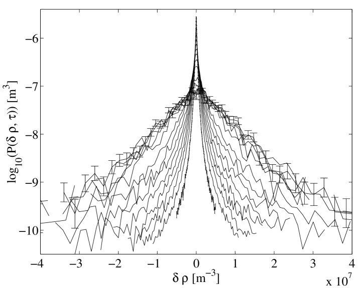
Figure 1: Unscaled PDFs of the ion density fluctuations. Time lag $\tau=2^{k}\times 46$s, where $k=0,1,2,..,14$. The standard deviation of the PDF increases with $\tau$. The error bars on each bin within the PDF are estimated assuming Gaussian statistics for the data within each bin.

Here, we apply a model-independent and generic PDF rescaling technique to extract the scaling properties of the solar wind fluctuations directly from the data. The aim is to determine a set of plasma parameters that exhibit statistical self-similarity and to verify the nature of the PDF for their fluctuations. We consider the following bulk plasma parameters: magnetic field magnitude $B$, velocity magnitude $v$, ion density $\rho$, kinetic and magnetic energy density ($\rho v^{2}$ and $B^{2}$) and Poynting flux approximated by $vB^{2}$. Such an approximation of the Poynting flux assumes ideal MHD where $\mathbf{E}=\mathbf{v}\times\mathbf{B}$. We find that the PDFs of fluctuations in $\rho$, $B^{2}$, $\rho v^{2}$ and $vB^{2}$ exhibit mono-scaling for up to $10$ standard deviations, while $B$ and $v$ are clearly multi-fractal as found previously burlaga (15, 12).

The mono-scaling allows us to derive a Fokker-Planck equation that governs the dynamics of the fluctuations’ PDFs. The Fokker-Planck approach provides a point of contact between the statistical approach and the dynamical features of the system. This allows us to identify the functional form of the space dependent diffusion coefficient that describes the fluctuations of these quantities as well as to develop a diffusion model for the shape of their PDFs. We also consider a Castaing model where fluctuations are assumed to arise from a varying energy transfer rate $\epsilon$ in the nonlinear energy cascade, with Gaussian distribution for $\ln(\epsilon)$.

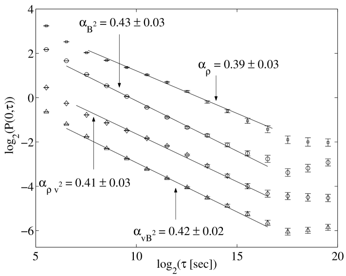
Figure 2: Scaling of the peaks $P(0,\tau)$ of the PDFs for all quantities under investigation: $\circ$ corresponds to $\delta B^{2}$, $\square$ ion density $\delta\rho$, $\diamond$ kinetic energy density $\delta(\rho v^{2})$ and $\triangle$ Poynting flux component $\delta(vB^{2})$. The plots have been offset vertically for clarity. Errors are estimated as in Fig. 1.

The paper is structured as follows: in section II we will describe the dataset used for this study as well as the rescaling procedure. In section III the results of the rescaling will be presented. Two possible models of the fluctuations will be discussed in Section IV. Finally in Section V we will summarize all results discussed throughout this paper.

II Data and Methods

II.1 The Dataset

The solar wind is a supersonic, super-Alfvénic flow of incompressible and inhomogeneous plasma. The WIND spacecraft orbits the Earth-Sun L1 point providing a set of in situ plasma parameters including magnetic field measurements from the MFI experiment lepping (16) and the plasma parameters from the SWE instrument ogilvie (17). The WIND solar wind magnetic field and key parameter database used here comprise over $1.5$ million, $46$ second averaged samples from January 1995 to December 1998 inclusive. The selection criteria for solar wind data is given by the component of the spacecraft position vector along the Earth-Sun line, $X>0$, and the vector magnitude, $R>30$ RE. The data set includes intervals of both slow and fast speed streams. Similar to other satellite measurements, short gaps in the WIND data file were present. To minimize the errors caused by such incomplete measurements we omitted any intervals where the gap was larger than $2\%$. The original data were not averaged nor detrended. The data are not sampled evenly but there are two dominant sampling frequencies: $1/46$ Hz and $1/92$ Hz. We use sampling frequency $f_{s}$ of $1/46$ as our base and treat other temporal resolutions as gaps when the accuracy requires it ($\tau\leq 92$ seconds).

II.2 Differencing and Rescaling Technique

Let $x(t)$ represent the time series of the studied signal, in our case magnetic field magnitude $B$, velocity magnitude $v$, ion density $\rho$, kinetic energy density $\rho v^{2}$, magnetic field energy density $B^{2}$ or the Poynting flux component approximated by $vB^{2}$. A set of time series $\delta x(t,\tau)=x(t+\tau)-x(t)$ is obtained for each value of the non-overlapping time lag $\tau$. The PDF $P(\delta x,\tau)$ is then generated for each time series $\delta x(t,\tau)$. Fig. 1 shows the set of such raw PDFs of the density fluctuations for time lags between $46$ seconds and $\sim 9$ days.

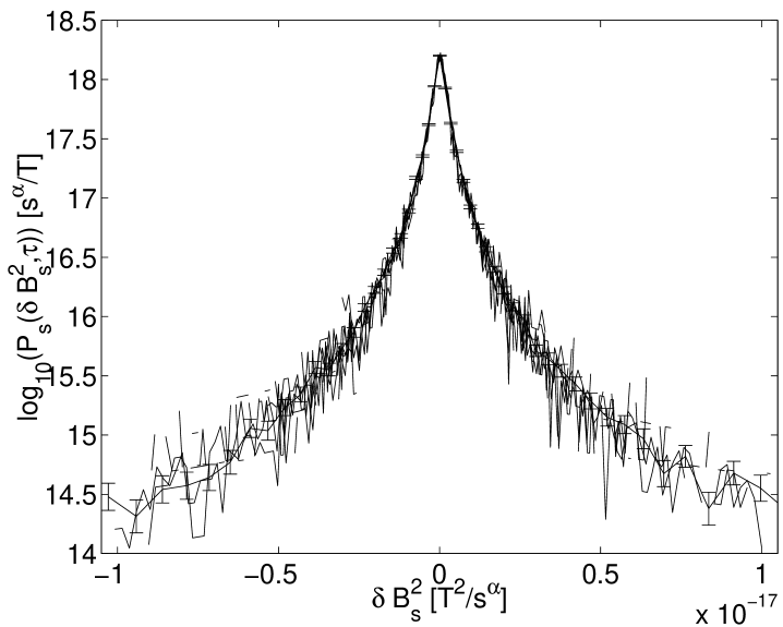
Figure 3: One parameter rescaling of the PDF for the fluctuations in the magnetic field energy density $B^{2}$. The curves shown correspond to $\tau$ between $~{}2$ minutes and $~{}26$ hours. Error bars as in Fig. 1.

A generic one parameter rescaling method hnat (14) is applied to these PDFs. We extract the scaling index $\alpha$, with respect to $\tau$, directly from the time series of the quantity $\delta x$. Practically, obtaining the scaling exponent relies on the detection of a power law, $P(0,\tau)\propto\tau^{-\alpha}$, for values of the raw PDF peaks and time lag $\tau$. Fig. 2 shows the peaks $P(0,\tau)$ of the unscaled PDFs plotted versus $\tau$ on log-log axes for the four bulk plasma parameters. We see that the peaks of these PDFs are well described by a power law $\tau^{-\alpha}$ for a range of $\tau$ up to $\sim 26$ hours. We now take $\alpha$ to be the scaling index and attempt to collapse all unscaled PDFs $P(\delta x,\tau)$ onto a single curve $P_{s}(\delta x_{s})$ using the following change of variables:

$$P(\delta x,\tau)=\tau^{-\alpha}P_{s}(\delta x\tau^{-\alpha}).$$ (1)

A self-similar Brownian walk with Gaussian PDFs on all temporal scales and index $\alpha=1/2$ is a good example of the process where such collapse can be observed (see e.g. sorn (18)). For experimental data, an approximate collapse of PDFs is an indicator of a dominant self-similar trend in the time series, i.e., this method may not be sensitive enough to detect multi-fractality that could be present only during short time intervals. One can treat the identification of the scaling exponent $\alpha$ and, as we will see, the non-Gaussian nature of the rescaled PDFs ($P_{s}$) as a method for quantifying the intermittent character of the time series. Another possible interpretation of the rescaling is to treat $P(\delta x,\tau)$ as the self-similar solution of the equation describing the PDF dynamics. The mono-scaling of the fluctuations PDF, together with the finite value of the samples’ variance, indicates that a Fokker-Planck approach can be used to express the dynamics of the unscaled PDF in time and with respect to the coordinate $\delta x$ kampen (19). In section $IV$ we will use the Fokker-Planck equation to develop a dynamical model for the fluctuations observed in the solar wind.

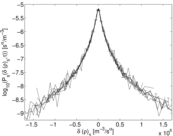
Figure 4: As in Fig. 3 for ion density fluctuations $\delta\rho$.

Ideally, we use the peaks of the PDFs to obtain the scaling exponent $\alpha$, as the peaks are statistically the most accurate parts of the distributions. In certain cases, however, the peaks may not be the optimal statistical measure for obtaining the scaling index. For example, the $B_{z}$ component of the solar wind magnetic field is measured with an absolute accuracy of typically about $0.1$ nT. Such discreteness in the time series introduces large errors in the estimation of the peak values $P(0,\tau)$ and may not give a correct scaling. However, if the PDFs rescale, we can in principle obtain the scaling exponent from any point on the curve. We will illustrate this in the next section where we obtain the rescaling index $\alpha$ from two points on the curve $P(0,\tau)$ and $P(\sigma,\tau)$.

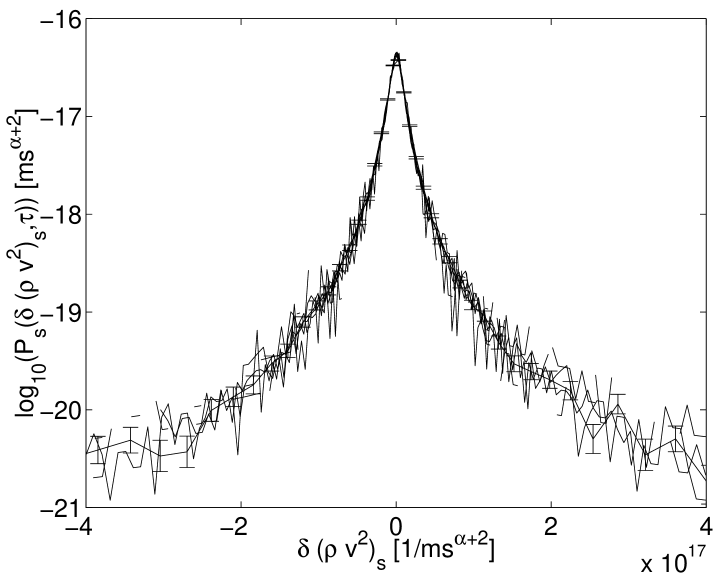
Figure 5: As in Fig. 3 for kinetic energy density fluctuations $\delta(\rho v^{2})$.

III PDF rescaling results

We are now ready to present results of the rescaling procedure as applied to the solar wind bulk plasma parameters. Fig. 1 shows the unscaled (raw) PDF curves of the ion density data. These PDFs, like all others presented in this section, were generated with the bin size decreasing linearly toward the center of the distribution to improve the accuracy of the PDF for small fluctuations. Although the entire range of data was used to create these PDFs we truncated the plotted curves for $|\delta x|\geq 10\sigma(\tau)$, where $\sigma(\tau)$ is a standard deviation of the differenced time series for the specific time lag $\tau$. Fig. 2 then shows $P(0,\tau)$ plotted versus $\tau$ on log-log axes for $\delta x=\delta(\rho)$, $\delta(\rho v^{2})$, $\delta(B^{2})$ and $\delta(vB^{2})$. Straight lines on such a plot suggest that the rescaling (1) holds at least for the peaks of the distributions. In Fig.  2, lines were fitted with $R^{2}$ goodness of fit for the range of $\tau$ between $~{}2$ minutes and $~{}26$ hours, omitting points corresponding to the first two temporal scales as in these cases the sharp peaks of the PDFs can not be well resolved. The lines suggest self-similarity persists up to intervals of $\tau\approx 26$ hours. The slopes of these lines yield the exponents $\alpha$ and these are summarized in Table 1 along with the values obtained from analogous plots of $P(\sigma(\tau),\tau)$ versus $\tau$ which show the same scale break and the same scaling exponent for $\delta(\rho)$, $\delta(\rho v^{2})$, $\delta(B^{2})$ and $\delta(vB^{2})$, to within the estimated statistical error.

Quantity	$\alpha$ from $P(0,\tau)$	$\alpha$ from $P(\sigma,\tau)$	Approx. $\tau_{max}$	PDF scales
$\delta B$	$-0.47\pm 0.02$	$-0.23\pm 0.05$	$~{}26$ hrs	No
$\delta v$	$-0.52\pm 0.05$	$-0.21\pm 0.06$	$~{}26$ hrs	No
$\delta(B^{2})$	$-0.43\pm 0.03$	$-0.39\pm 0.08$	$~{}26$ hrs	Yes
$\delta(\rho)$	$-0.39\pm 0.03$	$-0.37\pm 0.05$	$~{}26$ hrs	Yes
$\delta(\rho v^{2})$	$-0.41\pm 0.03$	$-0.35\pm 0.05$	$~{}26$ hrs	Yes
$\delta(vB^{2})$	$-0.42\pm 0.02$	$-0.39\pm 0.06$	$~{}26$ hrs	Yes

Table 1: Scaling indices derived from $P(0,\tau)$ and P($\sigma,\tau)$ power laws.

Within this scaling range we now attempt to collapse each corresponding unscaled PDF onto a single master curve using the scaling (1). Figs. 3-6 show the result of the one parameter rescaling applied to this unscaled PDF of fluctuations in $\rho$, $\rho v^{2}$, $B^{2}$ and $vB^{2}$ respectively, for temporal scales up to $\sim 26$ hours. We see that the rescaling procedure (1) using the value of the exponent $\alpha$ of the peaks $P(0,\tau)$ shown in Fig. 2, gives good collapse of each curve onto a single common functional form for the entire range of the data. These rescaled PDFs are leptokurtic rather than Gaussian and are thus strongly suggestive of an underlying nonlinear process.

The fluctuations PDFs for all mono-scaling quantities investigated here are nearly symmetric. This is in sharp contrast with the strong asymmetry of the PDF of velocity fluctuations in hydrodynamic turbulence reported previously in vainshtein (20, 10). This asymmetry of the statistics for the velocity increments coincides with the highly intermittent character of the flow and multi-fractal scaling of these fluctuations. We applied zeroth-order correlation functions, defined separately for the positive and the negative branch of the PDF vainshtein (20), to quantify the asymmetry of fluctuations PDFs for the solar wind. This analysis was performed using PDFs generated for $\tau\approx 12$ minutes (that is, within the scaling region). In the case of velocity increments we find that the negative moment is, on average, $11\%$ lower compared to the positive one. On the other hand, the quantities that we have found with self-similar increments do not have appreciable asymmetry. These show differences between negative and positive moments of about $2-3\%$, which is however, well above the statistical error of this procedure.

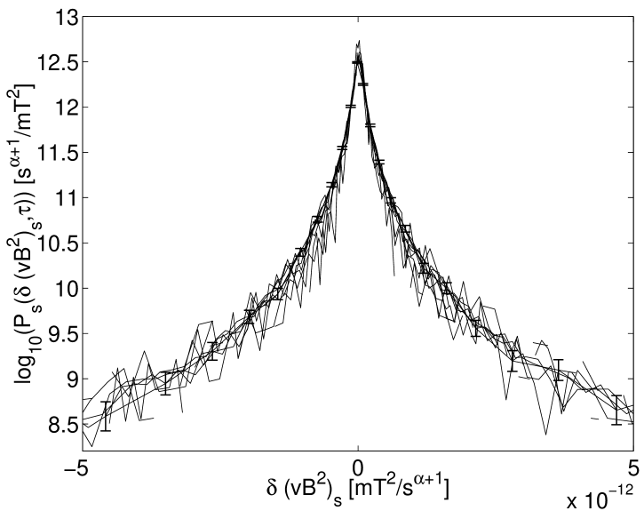
Figure 6: As in Fig. 3 for Poynting flux $\delta(vB^{2})$.

It has been reported previously castaing (10) that the PDFs obtained from hydrodynamic turbulence have exponential tails. These would look linear on the linear-log plots that are used in this paper. In the case of solar wind bulk plasma parameters we do not find such a clear exponential cutoff region but rather see stretched exponential tails of the form $P(|\delta x|)\sim\exp(-A|\delta x|^{\mu})$. This is illustrated in Fig. 7 where we plot $\log(\log(P(\delta x)))$ against $\log(\delta x)$ for all positive fluctuations of the mono-scaling quantities. It can be seen that, as we move away from the peak, these curves converge to lines and good fits can be obtained in the interval $[2\sigma,10\sigma]$, where $\sigma$ stands for the standard deviation.

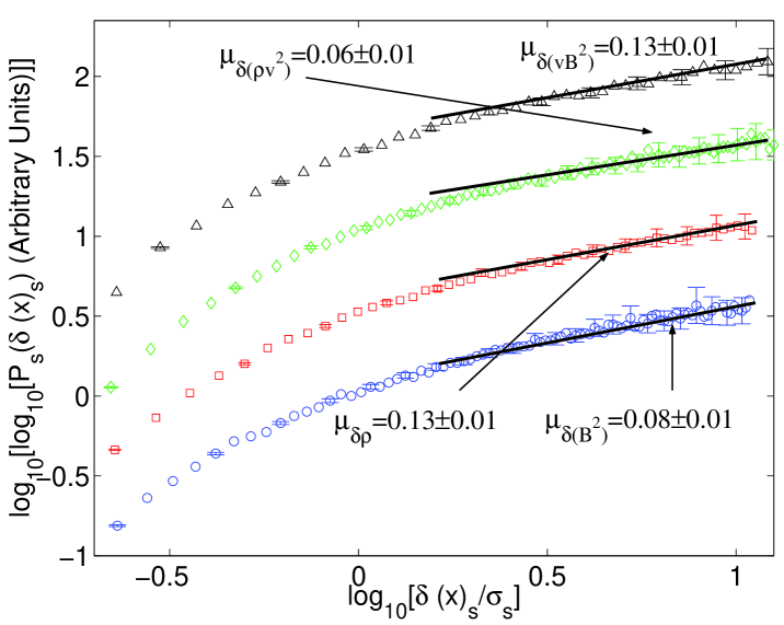
Figure 7: Positive tails of all self-similar PDFs for $\tau\approx 30$ minutes. Solid lines show linear fits obtained in the interval $[3\sigma,6\sigma]$ and extended to $[2\sigma,10\sigma]$ fluctuations interval.

We can now directly compare the functional form of these rescaled PDFs by normalizing the curves and overlying them on the single plot for a particular $\tau$ within the scaling range. Fig. 8 shows these normalized PDFs $P_{s}(\delta x_{s},\tau)$ for $\delta x_{s}=\delta(\rho)_{s}$, $\delta(B^{2})_{s}$, $\delta(\rho v^{2})_{s}$, $\delta(vB^{2})_{s}$ and $\tau\approx 1$ hour overlaid on a single plot. The $\delta x_{s}$ variable has been normalized to the rescaled standard deviation $\sigma_{s}(\tau\approx 1hr)$ of $P_{s}$ and the values of the PDF has been modified to keep probability constant in each case to facilitate this comparison. These normalized PDFs have remarkably similar functional form suggesting a shared process responsible for fluctuations in these four plasma parameters on temporal scales up to $\tau_{max}\approx 26$ hours.

It has been found previously burlaga (15) that the magnetic field magnitude fluctuations are not self-similar but rather multi-fractal. For such processes the scaling derived from $P(0,\tau)$ would not be expected to rescale the entire PDF. To verify this we applied the rescaling procedure for magnetic field magnitude differences $\delta B(t,\tau)=B(t+\tau)-B(t)$. Fig. 9 shows the result of one parameter rescaling applied to the PDFs of the magnetic field magnitude fluctuations. We see that the scaling procedure is satisfactory only up to $\sim 3$ standard deviations of the original sample, despite the satisfactory scaling obtained for the peaks $P(0,\tau)$ of the PDFs (see insert of the Fig. 9). This confirms the results of valvo (11) where a two parameter Castaing fit to values within $3$ standard deviations of the original sample yields scaling in one parameter and weak variation in the other. Attempts to improve the collapse by using information in the tails (values $|\delta B|>3\sigma$) would introduce a significant error in the estimation of the scaling exponent $\alpha$. We found similar lack of scaling in the fluctuations of the solar wind velocity magnitude and we show the rescaled PDF in the Fig. 10. We stress that the log-log plots of the PDF peaks $P(0,\tau)$ show a linear region for both velocity and magnetic field magnitude fluctuations (see insert in each figure). Their PDFs, however, do not collapse onto a single curve when the rescaling (1) is applied. This lack of mono-scaling is evident when indices derived from $P(0,\tau)$ and these found for $P(\sigma,\tau)$ are compared (see Table 1).

IV Modelling the data

The rescaling technique applied in the previous section indicates that, for certain temporal scales, the PDFs of some bulk plasma parameters can be collapsed onto a single master curve. The challenge now lays in developing physical models that can describe the functional form of this curve. Here we consider two approaches. The first is a statistical approach where we assume that the fluctuations can be described by a stochastic Langevin equation. The second method is to assume the fluctuations are the result of the nonlinear energy cascade and derive the corresponding PDF form for the rescaled PDFs (Castaing distribution) castaing (10).

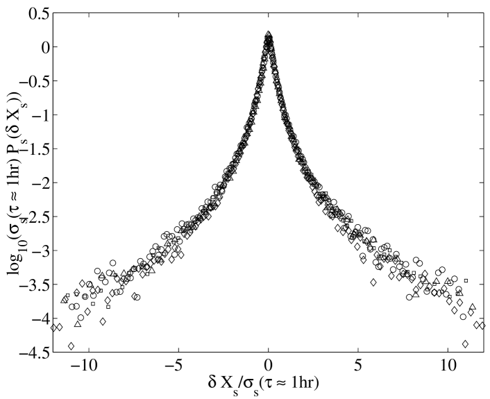
Figure 8: Direct comparison of the PDFs of fluctuations for all four quantities. $\circ$ corresponds to $\delta(B^{2})$, $\square$ ion density $\delta(\rho$), $\diamond$ kinetic energy density $\delta(\rho v^{2})$ and $\triangle$ Poynting flux component $\delta(vB^{2})$.

IV.1 Diffusion model

The Fokker-Planck (F-P) equation provides an important link between statistical studies and the dynamical approach expressed by the Langevin equation sorn (18). In the most general form F-P can be written as:

$$\frac{\partial{P}}{\partial{\tau}}=\nabla_{\delta x}(A(\delta x)P+B(\delta x)\nabla_{\delta x}P),$$ (2)

where $P\equiv P(\delta x,\tau)$ is a PDF for the differenced quantity $\delta x$ that varies with time $\tau$, $A(\delta x)$ is the friction coefficient and $B(\delta x)$ is related to a diffusion coefficient which we allow to vary with $\delta x$. For certain choices of $A(\delta x)$ and $B(\delta x)$, a class of self-similar solutions of (2) satisfies the rescaling relation given by (1). This scaling is a direct consequence of the fact that the F-P equation is invariant under the transformation $\delta x\rightarrow\delta x\tau^{-\alpha}$ and $P\rightarrow P\tau^{\alpha}$.

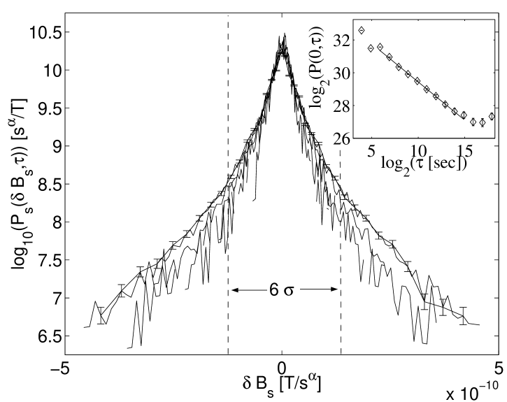
Figure 9: As in Fig. 3 for the solar wind magnetic filed magnitude fluctuations.

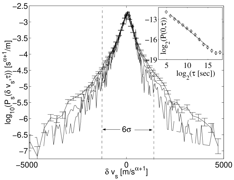
Figure 10: As in Fig. 3 for the solar wind velocity fluctuations.

It can be shown (see Appendix A) that equations (1) and (2) combined with power law scaling of the transport coefficients $A(\delta x)$ and $B(\delta x)$ lead to the following equation for the PDF:

$$\frac{\partial{P}}{\partial{\tau}}=\frac{\partial}{\partial{(\delta x)}}\left[(\delta x)^{1-1/\alpha}\left(a_{0}P+b_{0}\delta x\frac{\partial{P}}{\partial{(\delta x)}}\right)\right],$$ (3)

where $a_{0}$ and $b_{0}$ are constants, $\alpha$ is the scaling index derived from the data and $P(\delta x)$ and $\delta x$ are unscaled PDF and fluctuations respectively. Written in this form equation (3) immediately allows us to identity the functional form of the diffusion coefficient, namely $D(\delta x)\propto(\delta x)^{2-1/\alpha}$. In Appendix A we show how (3) can also be expressed as:

$$\frac{b_{0}}{a_{0}}(\delta x_{s})\frac{dP_{s}}{d(\delta x_{s})}+P_{s}+\frac{\alpha}{a_{0}}(\delta x_{s})^{\frac{1}{\alpha}}P_{s}=C.$$ (4)

The partial differential equation (4) can be solved analytically and one arrives at the general solution in the form:

$$P_{s}(\delta x_{s})=\frac{a_{0}}{b_{0}}\frac{C}{|\delta x_{s}|^{a_{0}/b_{0}}}exp\left(-\frac{\alpha^{2}}{b_{0}}(\delta x_{s})^{1/\alpha}\right)$$

$$\times\int_{0}^{\delta x_{s}}\frac{exp\left(\frac{\alpha^{2}}{b_{0}}(\delta x_{s}^{\prime})^{1/\alpha}\right)}{(\delta x_{s}^{\prime})^{1-a_{0}/b_{0}}}d(\delta x_{s}^{\prime})+k_{0}H(\delta x_{s}),$$ (5)

where $k_{0}$ is a constant and $H(\delta x_{s})$ is the homogeneous solution:

$$H(\delta x_{s})=\frac{1}{(\delta x_{s})^{a_{0}/b_{0}}}exp\left(-\frac{\alpha^{2}}{b_{0}}(\delta x_{s})^{1/\alpha}\right).$$ (6)

We then attempt to fit the predicted solution (5) to the normalized rescaled PDFs. The results of such a fit for the fluctuations of the kinetic energy density PDF is shown in Fig. 11 (solid line). This fit is obtained with the following parameters $a_{0}/b_{0}=2.0$, $b_{0}=10$, $C=0.00152$, $k_{0}=0.0625$ and $\alpha=0.41$ as derived from the rescaling procedure. We note that the figure is a semi-log plot and thus emphasizes the tails of the distribution - for a different value of the ratio $a_{0}/b_{0}$ the fit around the smallest fluctuations could be improved. Equation (5) can not, however, properly model the smallest fluctuations as it diverges for $\delta x_{s}\rightarrow 0$.

Let us now assume that a Langevin equation in the form

$$\frac{d(\delta x)}{dt}=\beta(\delta x)+\gamma(\delta x)\xi(t)$$ (7)

can describe the dynamics of the fluctuations. In (7) the random variable $\xi(t)$ is assumed to be $\delta$-correlated, i.e.,

$$<\xi(t)\xi(t+\tau)>=\sigma^{2}\delta(\tau).$$ (8)

This condition is fulfilled in the data analysis by forming each time series $\delta x(t,\tau)$ with non-overlapping time intervals $\tau$ and was also verified by computing the autocorrelation function of the differenced time series. Introducing a new variable $z=\int_{0}^{\delta x}1/\gamma(\delta x^{\prime})d(\delta x^{\prime})$, equation (7) can be written as:

$$\frac{dz}{dt}=\frac{\beta(z)}{\gamma(z)}+\xi(t).$$ (9)

One can immediately obtain a F-P equation that corresponds to the Langevin equation (9) kampen (19). We can then compare this F-P equation with that given by (3) to express coefficients $\beta(\delta x)$ and $\gamma(\delta x)$ in terms of $a_{0}$ and $b_{0}$ (see Appendix B). Defining $D_{0}=<\xi^{2}(t)>/2$ we obtain:

$$\gamma(\delta x)=\sqrt{\frac{b_{0}}{D_{0}}}(\delta x)^{1-\frac{1}{2\alpha}},$$ (10)

and

$$\beta(\delta x)=[b_{0}(1-\frac{1}{2\alpha})-a_{0}](\delta x)^{1-\frac{1}{\alpha}}.$$ (11)

Equation (7) together with definitions of its coefficients (10) and (11) constitutes a dynamical model for the fluctuations in the solar wind quantities. From (10) and (11), we see that the diffusion of the PDF of fluctuations in the solar wind is of comparable strength to the advection ($a_{0}/b_{0}\approx 2$). We stress that the advection and diffusion processes that we discuss here are of the probability in parameter space for fluctuations and do not refer to the integrated quantities.

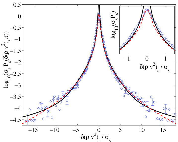
Figure 11: Example of the fit of the PDF functional form predicted by a Fokker-Planck description (5) (solid line) and a Castaing model (dash line) to the fluctuations PDF of the $\delta(\rho v^{2})$ bulk parameter.

IV.2 Castaing model

We now, for comparison, consider a model motivated directly by a cascade in energy, due to Castaing. This empirical model was developed for the spatial velocity fluctuations recorded from controlled experiments in wind tunnels castaing (10, 21) and has been applied to the solar wind data valvo (11, 12). The underlying idea of this approach is that, for constant energy transfer rate between spatial scales, all quantities should exhibit a Gaussian distribution of fluctuations. The intermittency is then introduced to the PDF through the fluctuations of the variance $\sigma$ of that Gaussian distribution. A log-normal distribution is assumed for the variance $\sigma$:

$$Q(\sigma)=\frac{1}{\sqrt{2\pi}\lambda}exp\left(-\frac{ln^{2}(\sigma/\sigma_{0})}{2\lambda^{2}}\right)d(ln(\sigma)),$$ (12)

where $\sigma_{0}$ is the most probable variance of the fluctuations and $\lambda$ is the variance of $ln(\sigma)$. Combining these two hypothesis Castaing proposed the following functional form for the observed PDF:

$$P_{\lambda}(\delta x)=\frac{1}{2\pi\lambda}\int_{0}^{\infty}exp\left(-\frac{(\delta x)^{2}}{2\sigma^{2}}\right)exp\left(-\frac{ln^{2}(\sigma/\sigma_{0})}{2\lambda^{2}}\right)\frac{d\sigma}{\sigma^{2}}.$$ (13)

The dashed line in the Fig. 11 shows the Castaing curve fitted with parameters $\lambda=1.275$ and $\sigma_{0}=0.225$ to the $\delta(\rho v^{2})$ PDF.

We can now compare the rescaled PDFs with both F-P and Castaing predicted curves which are shown in Fig. 11. We can see from the figure that both models provide an adequate fit to the $\delta(\rho v^{2})_{s}$ PDF, and hence will also describe the PDF of other scaling bulk plasma parameters. Both curves, however, fall significantly below observed PDF values for $|\delta(\rho v^{2})_{s}|\leq 2$, although the Castaing distribution fits the peak of the PDF reasonably well (see insert in Fig. 11). This departure from the experimental PDF, in the case of the Castaing distribution, may reflect the difference between hydrodynamics and MHD turbulence.

V Summary

In this paper we have applied a generic PDF rescaling method to fluctuations in the solar wind bulk plasma parameters. We find that, consistent with previous work, magnetic field and velocity magnitude fluctuations are multi-fractal whereas the PDFs of fluctuations in $B^{2}$, $\rho$, $\rho v^{2}$ and $vB^{2}$ can be rescaled with just one parameter for temporal scales up to $\sim 26$ hours. The presence of intermittency in the plasma flow is manifested in these quantities simply by the leptokurtic nature of their fluctuation PDFs, which show increased probability of large fluctuations compared to that of the Normal distribution. Fluctuations on large temporal scales, $\tau>26$ hours are uncorrelated in that their PDFs converge toward a Gaussian distribution. The fact that all quantities share the same PDF, to within errors, is also strongly suggestive of a single underlying process. This is also supported by the similar values of the scaling exponents.

The simple scaling properties that we have found allow us to develop a Fokker-Planck approach which provides a functional form of the rescaled PDFs as well as a Langevin equation for the dynamics of the observed fluctuations. The model shows that both advective and diffusive terms need to be invoked to describe the dynamics of the fluctuations. The calculated diffusion coefficient is of the form $D(x_{s})\propto(\delta x_{s})^{2-1/\alpha}$. We obtained a good fit of the model to our rescaled PDFs over at least $10$ standard deviations. We also examined a Castaing model for turbulence and found a set of fit parameters for which both the Castaing distribution and our diffusion model have nearly identical form. Since both the F-P model and the Castaing distribution fit our rescaled PDFs we conclude that their moments should exhibit same variation with time lag $\tau$.

VI Acknowledgment

S. C. Chapman and B. Hnat acknowledge support from the PPARC and G. Rowlands from the Leverhulme Trust. We thank N. W. Watkins and M. P. Freeman for advice concerning the post processing of the WIND data. We also thank R.P Lepping and K. Ogilvie for provision of data from the NASA WIND spacecraft.

Appendix A

Let $P(\delta x,\tau)$ be a homogeneous function that satisfies scaling (1). Our aim is to find functional form of the coefficients $A(\delta x)$ and $B(\delta x)$ for which $P(\delta x,\tau)$ is a solution of a F-P equation (2). Using (1) we can now rewrite (2) to read:

$$-\frac{\alpha}{t^{\alpha+1}}\left(P_{s}+\delta x_{s}\frac{dP_{s}}{d(\delta x_{s})}\right)=\frac{P_{s}}{t^{\alpha}}\frac{dA(\delta x)}{d(\delta x)}+\frac{A(\delta x)}{t^{2\alpha}}\frac{dP_{s}}{d(\delta x_{s})}$$

$$+\frac{1}{t^{2\alpha}}\frac{dB(\delta x)}{d(\delta x)}\frac{dP_{s}}{d(\delta x_{s})}+\frac{B(\delta x)}{t^{3\alpha}}\frac{dP_{s}}{d(\delta x_{s})}.$$ (14)

If all terms in the rhs of (14) are to contribute and for $P(\delta x_{s})$ to remain a function of $\delta x_{s}$ only we must have:

$$\frac{A(\delta x)}{t^{\alpha-1}}=a(\delta x_{s})\quad\textrm{and}\quad\frac{B(\delta x)}{t^{2\alpha-1}}=b(\delta x_{s}).$$ (15)

Both $A(\delta x)$ and $B(\delta x)$ must then be of form:

$$A(\delta x)=a_{0}(\delta x)^{\eta}\quad\textrm{and}\quad B(\delta x)=b_{0}(\delta x)^{\nu},$$ (16)

where $a_{0}$ and $b_{0}$ are constants. Changing variables to the rescaled $\delta x_{s}$ and substituting (16) into (15) we express exponents $\eta$ and $\nu$ in terms of the rescaling index $\alpha$ derived from the data. We then obtain:

$$\eta=1-\frac{1}{\alpha}\quad\textrm{and}\quad\nu=2-\frac{1}{\alpha},$$ (17)

which allows to write the final power law form of $A(\delta x)$ and $B(\delta x)$:

$$A(\delta x)=a_{0}(\delta x)^{1-\frac{1}{\alpha}}\quad\textrm{and}\quad B(\delta x)=b_{0}(\delta x)^{2-\frac{1}{\alpha}}.$$ (18)

Substituting these expressions into F-P equation (2) we obtain (3) from Section $4$. Using these results the term $\frac{dA(\delta x)}{d(\delta x)}$ on the rhs of (14), for example, becomes:

$$\frac{dA(\delta x)}{d(\delta x)}=\left(1-\frac{1}{\alpha}\right)a_{0}(\delta x)^{-\frac{1}{\alpha}}.$$ (19)

Performing similar algebra on all terms in (14) we arrive to equation:

$$-\alpha\frac{d(\delta x_{s}P_{s})}{d(\delta x_{s})}=\frac{d}{d(\delta x_{s})}\left[(\delta x_{s})^{1-\frac{1}{\alpha}}\left(a_{0}P_{s}+b_{0}(\delta x_{s})\frac{dP_{s}}{d(\delta x_{s})}\right)\right].$$ (20)

Integrated once we obtain equation (4)

$$\frac{b_{0}}{a_{0}}(\delta x_{s})\frac{dP_{s}}{d(\delta x_{s})}+P_{s}+\frac{\alpha}{a_{0}}(\delta x_{s})^{\frac{1}{\alpha}}dP_{s}=C,$$ (21)

where $C$ is the constant of integration.

Appendix B

Consider the following Langevin type of equation:

$$\frac{d(\delta x)}{dt}=\beta(\delta x)+\gamma(\delta x)\xi(t),$$ (22)

where the random variable $\xi(t)$ is assumed to be $\delta$-correlated, i.e.,

$$<\xi(t)\xi(t+\tau)>=\sigma^{2}\delta(\tau).$$ (23)

Introducing a new variable $z=\int_{0}^{\delta x}1/\gamma(\delta x^{\prime})d(\delta x^{\prime})$, equation (22) can be written as:

$$\frac{dz}{dt}=\Gamma(z)+\xi(t),\quad\textrm{where}\quad\Gamma(z)=\frac{\beta(z)}{\gamma(z)}.$$ (24)

One can immediately obtain a F-P equation that corresponds to the Langevin equation (24) and reads:

$$\frac{\partial{P(z,\tau)}}{\partial{\tau}}+\frac{\partial}{\partial{z}}\left(\Gamma(z)P(z,\tau)\right)=D_{0}\frac{\partial^{2}{P(z,\tau)}}{\partial^{2}{z}},$$ (25)

where $D_{0}=\sigma^{2}/2$. The probability is an invariant of the variable change so that $P(\delta x)d(\delta x)=P(z)dz$ and we can then rewrite (25) for $P(\delta x,\tau)$:

$$\frac{\partial{P}}{\partial{\tau}}=\frac{\partial}{\partial{(\delta x)}}\left[\left(D_{0}\gamma(\delta x)\frac{d\gamma(\delta x)}{d(\delta x)}-\beta(\delta x)\right)P+D_{0}\gamma^{2}\frac{\partial{P}}{\partial{(\delta x)}}\right].$$ (26)

Comparing (26) with the F-P equation (3) we can identify:

$$D_{0}\gamma^{2}=(\delta x)^{1-\frac{1}{\alpha}}b_{0}\delta x,$$ (27)

and then we must demand that:

$$\frac{D_{0}}{2}\frac{d\gamma^{2}(\delta x)}{d(\delta x)^{2}}-\beta(\delta x)=a_{0}(\delta x)^{1-\frac{1}{\alpha}}.$$ (28)

In summary we have shown that the F-P equation given by (3) is equivalent to the stochastic Langevin equation (7) where coefficients $\beta$ and $\gamma$ are given by:

$$\gamma=\sqrt{\frac{b_{0}}{D_{0}}}(\delta x)^{1-\frac{1}{2\alpha}},$$ (29)

and

$$\beta=\left[b_{0}\left(1-\frac{1}{2\alpha}\right)-a_{0}\right](\delta x)^{1-\frac{1}{\alpha}}.$$ (30)

References

- (1) V. Carbone, P. Veltri and R. Bruno, Phys. Rev. Lett. 75, 3110–3113 (1995).
- (2) P. Veltri, Plasma Phys. Control. Fusion 41, A787–A795 (1999).
- (3) T. Bohr, M. H. Jensen, G. Paladin and A. Vulpiani, Dynamical Systems Approach to Turbulence (Cambridge University Press, Cambridge, 1998).
- (4) U. Frisch, Turbulence. The legacy of A.N. Kolmogorov (Cambridge University Press, Cambridge, 1995).
- (5) C.-Y. Tu and E. Marsch, Space Sci. Rev. 73, 1-210 (1995).
- (6) M. L. Goldstein and D. A. Roberts, Phys. Plasmas 6, 4154–4160 (1999).
- (7) A.V. Milovanov and L. M. Zelenyi, Astrophys. Space Sci. 264, 317–345 (1998).
- (8) M. Dobrowolny, A. Mangeney and P. L. Veltri, Phys. Rev. Lett. 45, 144–147 (1980).
- (9) A.N. Kolmogorov, J. Fluid Mech. 13, 82–85 (1962).
- (10) B. Castaing, Y. Gagne and E. J. Hopfinger, Physica D 46, 177–200 (1990).
- (11) L. Sorriso-Valvo, V. Carbone, P. Giuliani, P. Veltri, R. Bruno, V. Antoni and E. Martines, Planet. Space Sci. 49, 1193–1200 (2001).
- (12) M. A. Forman and L. F. Burlaga, in Solar Wind Ten, edited by M. Velli, et al., (American Institute of Physics), (in press)
- (13) R. N. Mantegna & H. E. Stanley, Nature 376, 46–49 (1995).
- (14) B. Hnat, S. C. Chapman, G. Rowlands, N. W. Watkins, W. M. Farrell, Geophys. Res. Lett. 29(10), 10.1029/2001GL014587 (2002).
- (15) L. F. Burlaga, J. Geophys. Res. 106, 15,917–15,927 (2001).
- (16) R. P. Lepping et al., Space Sci. Rev. 71, 207 (1995).
- (17) K. W. Ogilvie et al., Space Sci. Rev. 71, 55–77 (1995).
- (18) D. Sornette, Critical Phenomena in Natural Sciences; Chaos, Fractals, Selforganization and Disorder: Concepts and Tools, (Springer-Verlag, Berlin, 2000).
- (19) N.G. van Kampen, Stochastic Processes in Physics and Chemistry, (North-Holland, Amsterdam, 1992).
- (20) S. I. Vainshtein, Phys. Rev. E 56, 447–461 (1997).
- (21) C. van Atta and J. T. Park, Lecture Notes in Physics, Vol. 12, edited by M. Rosenblatt and C. Van Atta, (Springer Verlag, Berlin, 1972), pp. 402-426.